
Luminance-Degradation Compensation Based on Multistream Self-Attention to Address Thin-Film Transistor-Organic Light Emitting Diode Burn-In


Abstract
:1. Introduction
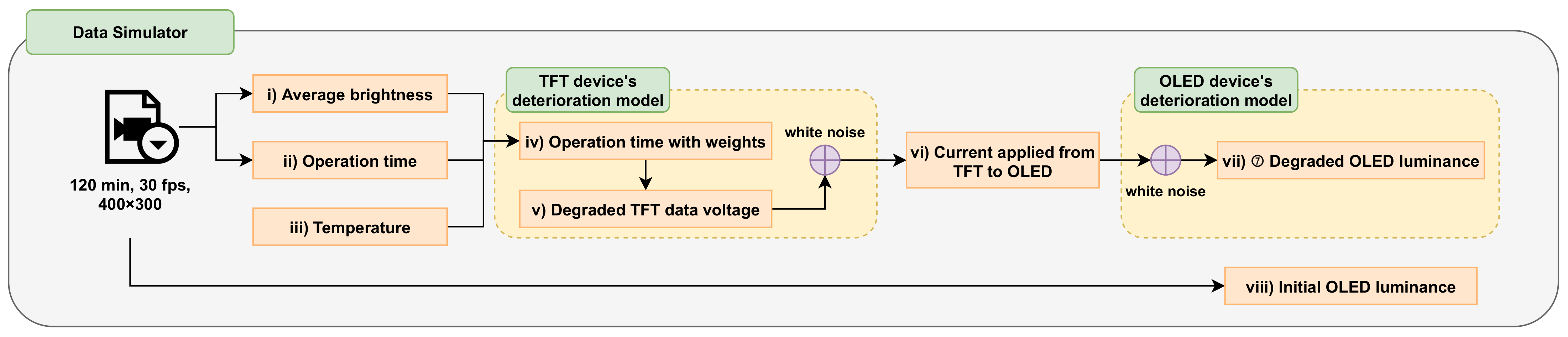
2. Data Simulator
- First, the data simulator outputs (i) the average brightness per pixel () and (ii) operation time () from the input video. It also adds (iii) a temperature condition (T) between 0 and 60 , which affects the deterioration of the TFT and OLED devices.
- The previously obtained variables are used to output (iv) the operation time with weights per pixel () and (v) the degraded TFT data voltage () with the change in time and temperature. White noise is also mixed to create conditions similar to real-world environments.
- is used for each time and temperature to output (vi) the degraded OLED current () of the TFT and to mix the white noise.
- (vii) Degraded OLED luminance () is observed using for each time and temperature. (viii) The initial OLED luminance () is obtained directly from the input video.
| Algorithm 1: Calculation of operating time per pixel. |
 |
3. Data Augmentation
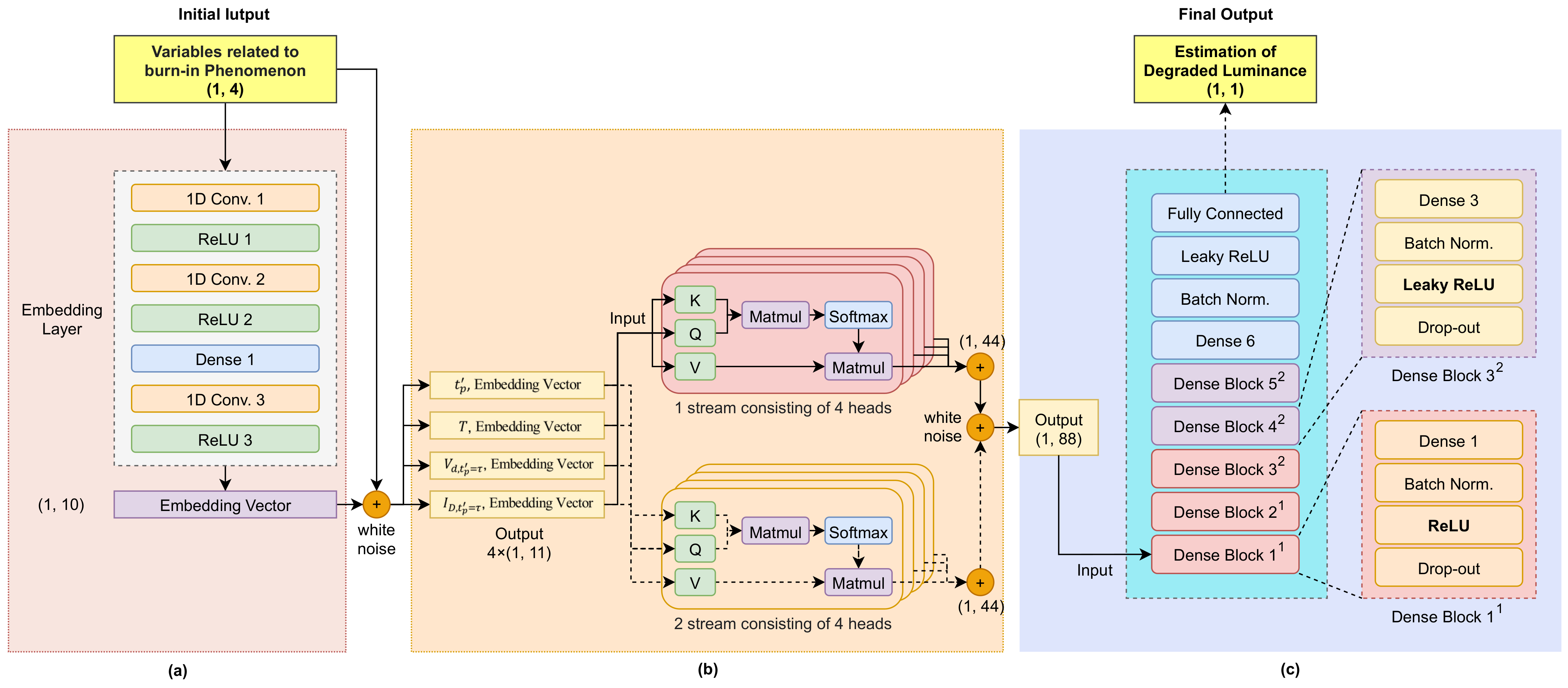
4. Deep-Learning Model
4.1. Data Configuration
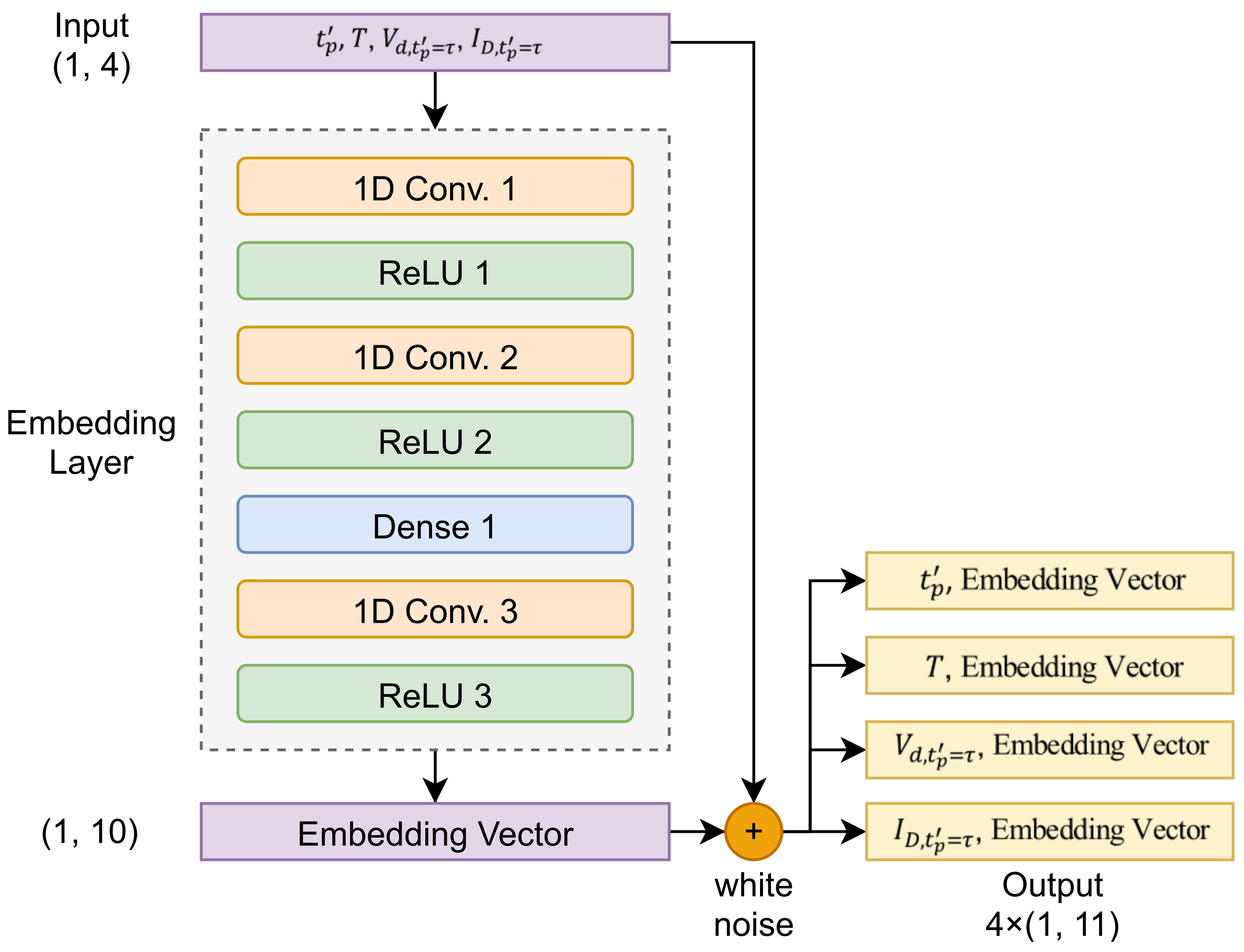
4.2. Deep-Feature Generation
4.3. Multistream Self-Attention
4.4. DNN
5. Experimental Environment and Result
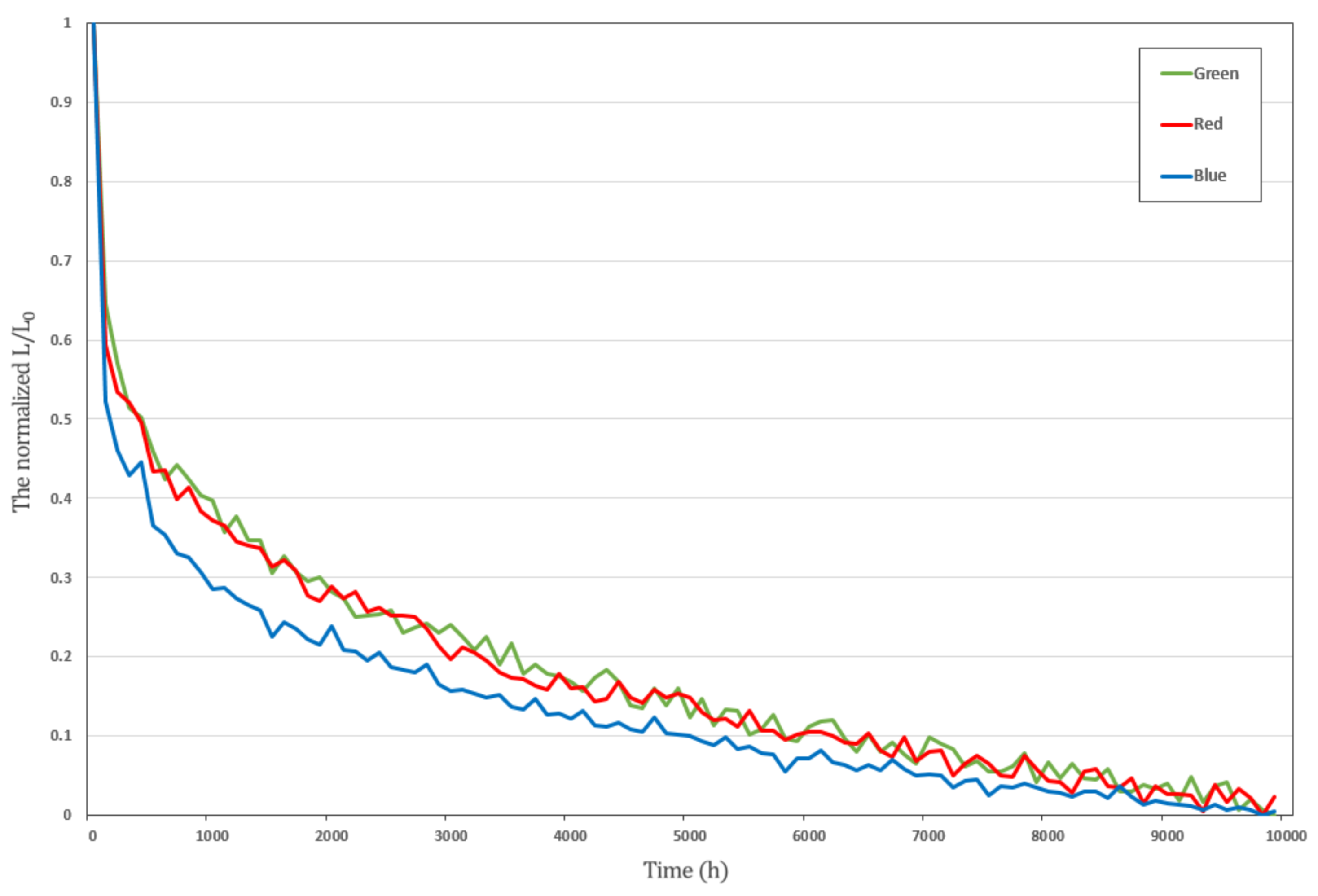
5.1. Datasets
5.2. Experiment Setup
5.3. Result Analysis
6. Conclusions
Author Contributions
Funding
Institutional Review Board Statement
Informed Consent Statement
Data Availability Statement
Conflicts of Interest
References
- Kang, S. OLED power control algorithm using optimal mapping curve determination. J. Disp. Technol. 2016, 12, 1278–1282. [Google Scholar] [CrossRef]
- Jung, H.; Kim, Y.; Chen, C.; Kanicki, J. A-IGZO TFT based pixel circuits for AM-OLED displays. Proc. SID Tech. Dig. 2012, 43, 1097–1100. [Google Scholar] [CrossRef]
- Wang, C.; Hu, Z.; He, X.; Liao, C.; Zhang, S. One gate diode-connected dual-gate a-IGZO TFT driven pixel circuit for active matrix organic light-emitting diode displays. IEEE Trans. Electron Devices 2016, 63, 3800–3803. [Google Scholar] [CrossRef]
- In, H.-J.; Kwon, O.-K. External compensation of nonuniform electrical characteristics of thin-film transistors and degradation of OLED devices in AMOLED displays. IEEE Electron Device Lett. 2009, 30, 377–379. [Google Scholar]
- Lee, K.-Y.; Chao, Y.-P.; Chen, W.-D. A new compensation method for emission degradation in an AMOLED display via an external algorithm, new pixel circuit, and models of prior measurements. J. Disp. Technol. 2014, 10, 189–197. [Google Scholar] [CrossRef]
- Xia, S.C.; Kwong, R.C.; Adamovich, V.I.; Weaver, M.S.; Brown, J.J. OLED device operational lifetime: Insights and challenges. In Proceedings of the 2007 IEEE 45th Annual International Reliability Physics Symposium, Phoenix, AZ, USA, 15–19 April 2007; pp. 253–257. [Google Scholar] [CrossRef]
- Zhou, X.; He, J.; Liao, L.S.; Lu, M.; Ding, X.M.; Hou, X.Y.; Zhang, X.M.; He, X.Q.; Lee, S.T. Real-time observation of temperature rise and thermal breakdown processes in organic LEDs using an IR imaging and analysis system. Adv. Mater. 2000, 12, 265–269. [Google Scholar] [CrossRef]
- Kundrata, J.; Baric, A. Electrical and thermal analysis of an OLED module. In Proceedings of the Comsol Conference, Milan, Italy, 10–12 October 2012. [Google Scholar]
- Kim, H.; Shin, H.; Park, J.; Choi, Y.; Park, J. Statistical modeling and reliability prediction for transient luminance degradation of flexible OLEDs. In Proceedings of the 2018 IEEE International Reliability Physics Symposium (IRPS), Burlingame, CA, USA, 11–15 March 2018; pp. 3C.7-1–3C.7-6. [Google Scholar] [CrossRef]
- Dong, M.; Choi, Y.K.; Zhong, L. Power modeling of graphical user interfaces on OLED displays. In Proceedings of the 2009 46th ACM/IEEE Design Automation Conference, San Francisco, CA, USA, 26–31 July 2009; pp. 652–657. [Google Scholar]
- Hadizadeh, H. Energy-Efficient Images. IEEE Trans. Image Process. 2017, 26, 2882–2891. [Google Scholar] [CrossRef] [PubMed]
- Chang, T.; Xu, S.S. Real-time quality-on-demand energy-saving schemes for OLED-based displays. In Proceedings of the 2013 IEEE International Symposium on Industrial Electronics, Taipei, Taiwan, 28–31 May 2013; pp. 1–5. [Google Scholar] [CrossRef]
- Scholz, S.; Kondakov, D.; Lussem, B.; Leo, K. Degradation mechanisms and reactions in organic light-emitting devices. Chem. Rev. 2015, 115, 8449–8503. [Google Scholar] [CrossRef]
- Langlois, E.; Wang, D.; Shen, J. Degradation mechanisms in organic light emitting diodes. Synth. Met. 2000, 111, 233–236. [Google Scholar]
- Schmidbauer, S.; Hohenleutner, A.; Konig, B. Chemical Degradation in Organic Light-Emitting Devices: Mechanisms and Implications for the Design of New Materials. Adv. Mater. 2013, 25, 2114–2129. [Google Scholar] [CrossRef]
- Fery, C.; Racine, B.; Vaufrey, D.; Doyeux, H.; Cina, S. Physical mechanism responsible for the stretched exponential decay behavior of aging organic light-emitting diodes. Appl. Phys. Lett. 2005, 87, 213502–213503. [Google Scholar] [CrossRef]
- Lee, K.-Y.; Hsu, Y.-P.; Chao, C.-P. A new 4T0.C AMOLED pixel circuit with reverse bias to alleviate OLED degradation. IEEE Electron Device Lett. 2012, 33, 1024–1026. [Google Scholar] [CrossRef]
- Lin, C.-L.; Chen, Y.-C. A novel LTPS-TFT pixel circuit compensating for TFT threshold-voltage shift and OLED degradation for AMOLED. IEEE Electron Device Lett. 2007, 28, 129–131. [Google Scholar] [CrossRef]
- Lee, K.-Y.; Chao, C.-P. A new AMOLED pixel circuit with pulsed drive and reverse bias to alleviate OLED degradation. IEEE Electron Device Lett. 2012, 59, 1123–1130. [Google Scholar] [CrossRef] [Green Version]
- Zeng, M.; Nguyen, L.T.; Yu, B.; Mengshoel, O.J.; Zhu, J.; Wu, P.; Zhang, J. Convolutional Neural Networks for human activity recognition using mobile sensors. In Proceedings of the 2014 6th International Conference on Mobile Computing, Applications and Services, Austin, TX, USA, 6–7 November 2014; pp. 197–205. [Google Scholar]
- Ravi, D.; Wong, C.; Lo, B.; Yang, G.-Z. A Deep Learning Approach to on-Node Sensor Data Analytics for Mobile or Wearable Devices. IEEE J. Biomed. Health Inform. 2017, 21, 56–64. [Google Scholar] [CrossRef] [PubMed] [Green Version]
- Krizhevsky, A.; Sutskever, I.; Hinton, G.E. Imagenet classification with deep convolutional neural networks. Adv. Neural Inf. Process. Syst. 2012, 25, 1097–1105. [Google Scholar] [CrossRef]
- Psuj, G. Degradation Mechanisms in Organic Light Emitting Diodes. Sensors 2018, 18, 292. [Google Scholar] [CrossRef] [Green Version]
- Zhang, J.; Li, W.; Cheng, G.; Chen, X.; Wu, H.; Shen, H. Life prediction of OLED for constant-stress accelerated degradation tests using luminance decaying model. Appl. Phys. Lett. 2014, 154, 491–495. [Google Scholar] [CrossRef]
- Taylor, L.; Nitschke, G. Improving Deep Learning using Generic Data Augmentation. arXiv 2017, arXiv:1708.06020v1. [Google Scholar]
- Bosch, S.V.D. Automatic Feature Generation and Selection in Predictive Analytics Solutions. Master’s Thesis, Faculty of Science, Radboud University, Nijmegen, The Netherlands, 2017. [Google Scholar]
- Agarap, F. Deep learning using rectified linear units (relu). arXiv 2018, arXiv:1803.08375. [Google Scholar]
- Kiranyaz, S. 1-D Convolutional Neural Networks for Signal Processing Applications. In Proceedings of the ICASSP 2019—2019 IEEE International Conference on Acoustics, Speech and Signal Processing (ICASSP), Brighton, UK, 12–17 May 2019; pp. 8360–8364. [Google Scholar]
- Han, K.J.; Prieto, R. State-of-the-art speech recognitions using multi-stream self-attention with dilated 1D convolutions. arXiv 2019, arXiv:1910.00716v1. [Google Scholar]
- Vaswani, A.; Shazeer, N.; Parmar, N.; Uszkoreit, J.; Jones, L.; Gomez, A.N.; Kaiser, Ł.; Polosukhin, I. Attention is all you need. In Proceedings of the Advances in Neural Information Processing Systems 30 (NIPS 2017), Long Beach, CA, USA, 4–9 December 2017; pp. 5998–6008. [Google Scholar]
- Heaton, J.; Goodfellow, I.; Bengio, Y.; Courville, A. Deep learning. Genet. Program. Evolvable Mach. 2018, 19, 305–307. [Google Scholar] [CrossRef] [Green Version]
- Yeh, C.-H. Visual-Attention-Based Pixel Dimming Technique for OLED Displays of Mobile Devices. IEEE Trans. Ind. Electron. 2019, 66, 7159–7167. [Google Scholar] [CrossRef]
- Ioffe, S.; Szegedy, C. Batch Normalization: Accelerating Deep Network Training by Reducing Internal Covariate Shift. Available online: https://arxiv.org/pdf/1502.03167.pdf (accessed on 19 September 2019).
- Kingma, D.P.; Ba, J. Adam: A Method for Stochastic Optimization. Available online: https://arxiv.org/pdf/1412.6980.pdf (accessed on 19 September 2019).


| Contents | Specifications |
|---|---|
| Content 1 (40 min) | Documentary, action, news, sports |
| Content 2 (40 min) | Entertainment, beauty, animation, car review |
| Content 3 (40 min) | Game, cooking, job introduction, romance |
| Symbol | Parameter | Symbol | Parameter |
|---|---|---|---|
| Data of input video | N | Total frame of input video | |
| f | Frame | P | Total pixel |
| p | Pixel | t | Time |
| Operating time per pixel | Weighted operating time | ||
| Brightness of per pixel | Average brightness per pixel | ||
| Noise of threshold voltage | Noise of mobility | ||
| Reduction factor of shifting value of threshold voltage | Reduction factor of threshold voltage | ||
| Reduction factor of mobility | Maximum input current of TFT | ||
| L | Length of TFT channel | W | Width of TFT channel |
| Data voltage of TFT that consider noise | Initial data voltage of TFT | ||
| Capacitor of TFT unit area | Initial mobility of TFT | ||
| Threshold voltage of TFT that consider noise | Drain voltage of TFT | ||
| Maximal temperature of TFT performance guarantee | Shifting value of threshold voltage | ||
| Initial threshold voltage of TFT | w | Weight factor | |
| n | Gray level of TFT | l | Total gray level range |
| Reduction rate of OLED voltage | T | Temperature | |
| Transistor parameter | Gate capacitor | ||
| W | Channel width |
| Datasets | Train/Test | Total |
|---|---|---|
| OLED pixel (Blue) | 9.72/1.08 billion | 10.8 billion |
| Experiment 1 | Experiment 2 | Experiment 3 | ||||
|---|---|---|---|---|---|---|
| Experimental Details | Layers | Kernel Filter Size Units | Layers | Kernel Filter Size Units | Layers | Kernel, Filter Size Units |
| 1D Conv 1 | 1 × 4 @32 | 1D Conv 1 | 1 × 4 @32 | 1D Conv 1 | 1 × 4 @32 | |
| 1D Conv 2 | 1 × 32 @16 | 1D Conv 2 | 1 × 32 @16 | Dense 1 | 32 | |
| Dense 1 | 16 | Dense 1 | 16 | 1D Conv 2 | 1 × 32 @16 | |
| 1D Conv 3 | 1 × 16 @10 | Dense 2 | 16 | |||
| 1D Conv 3 | 1 × 16 @10 | |||||
| Accuracy | 90.28% | 91.62% | 91.45% | |||
| Experimental Details | Experiment 1 | Experiment 2 |
|---|---|---|
| 1-Stream Self-Attention | 2-Stream Self-Attention | |
| Accuracy | 90.75% | 92.19% |
| Experiment 1 | Experiment 2 | Experiment 3 | ||||
|---|---|---|---|---|---|---|
| Layer Number | Units | Layer Number | Units | Layer Number | Units | |
| Experimental Details | Dense layer 1 | 64 | Dense layer 1 | 64 | Dense layer 1 | 64 |
| Dense layer 2 | 64 | Dense layer 2 | 64 | Dense layer 2 | 64 | |
| Dense layer 3 | 64 | Dense layer 3 | 64 | Dense layer 3 | 64 | |
| Dense layer 4 | 64 | Dense layer 4 | 64 | Dense layer 4 | 64 | |
| Dense layer 5 | 64 | Dense layer 5 | 64 | |||
| Dense layer 6 | 64 | |||||
| Accuracy | 89.94% | 91.22% | 93.31% | |||
| Layer Number | Experiment 1 | Experiment 2 | Experiment 3 | Experiment 4 | Experiment 5 | |
|---|---|---|---|---|---|---|
| Units | ||||||
| Experiment Details | Dense layer 1 | 64 | 128 | 256 | 256 | 256 |
| Dense layer 2 | 64 | 128 | 256 | 128 | 128 | |
| Dense layer 3 | 64 | 128 | 256 | 128 | 128 | |
| Dense layer 4 | 64 | 128 | 256 | 256 | 256 | |
| Dense layer 5 | 64 | 128 | 256 | 128 | 128 | |
| Dense layer 6 | 64 | 128 | 256 | 64 | 128 | |
| Accuracy | 92.58% | 93.35% | 93.76% | 95.44% | 95.10% | |
Publisher’s Note: MDPI stays neutral with regard to jurisdictional claims in published maps and institutional affiliations. |
© 2021 by the authors. Licensee MDPI, Basel, Switzerland. This article is an open access article distributed under the terms and conditions of the Creative Commons Attribution (CC BY) license (https://creativecommons.org/licenses/by/4.0/).
Share and Cite
Park, S.-C.; Park, K.-H.; Chang, J.-H. Luminance-Degradation Compensation Based on Multistream Self-Attention to Address Thin-Film Transistor-Organic Light Emitting Diode Burn-In. Sensors 2021, 21, 3182. https://doi.org/10.3390/s21093182
Park S-C, Park K-H, Chang J-H. Luminance-Degradation Compensation Based on Multistream Self-Attention to Address Thin-Film Transistor-Organic Light Emitting Diode Burn-In. Sensors. 2021; 21(9):3182. https://doi.org/10.3390/s21093182
Chicago/Turabian StylePark, Seong-Chel, Kwan-Ho Park, and Joon-Hyuk Chang. 2021. "Luminance-Degradation Compensation Based on Multistream Self-Attention to Address Thin-Film Transistor-Organic Light Emitting Diode Burn-In" Sensors 21, no. 9: 3182. https://doi.org/10.3390/s21093182