
Semantic Point Cloud Segmentation Using Fast Deep Neural Network and DCRF †

Abstract
:1. Introduction
- A point cloud reduction and feature extraction method that allows a large-scale reduction of the number of point clouds in a scene and generation of a series of ordered features of the point cloud.
- Improved PointNet network structure is used to allow the new network structure to perform the task, and introduced a new loss function to improve the accuracy of the network.
- A new DenseCRF functional model is proposed to make full use of the semantic classification result model to optimize the network segmentation results.
2. Related Work
2.1. 3D Data Representation
2.2. Semantic Segmentation
2.3. DenseCRF
3. New Network Structure for Semantic Point Cloud Segmentation
3.1. Point Cloud Mapping and Feature Extension
3.2. New Neural Network for Semantics Segmentation
3.3. Improving Segmentation with DenseCRF
4. Evaluation and Comparison
4.1. Network Establishment and Preprocessing
4.2. Implementation Details
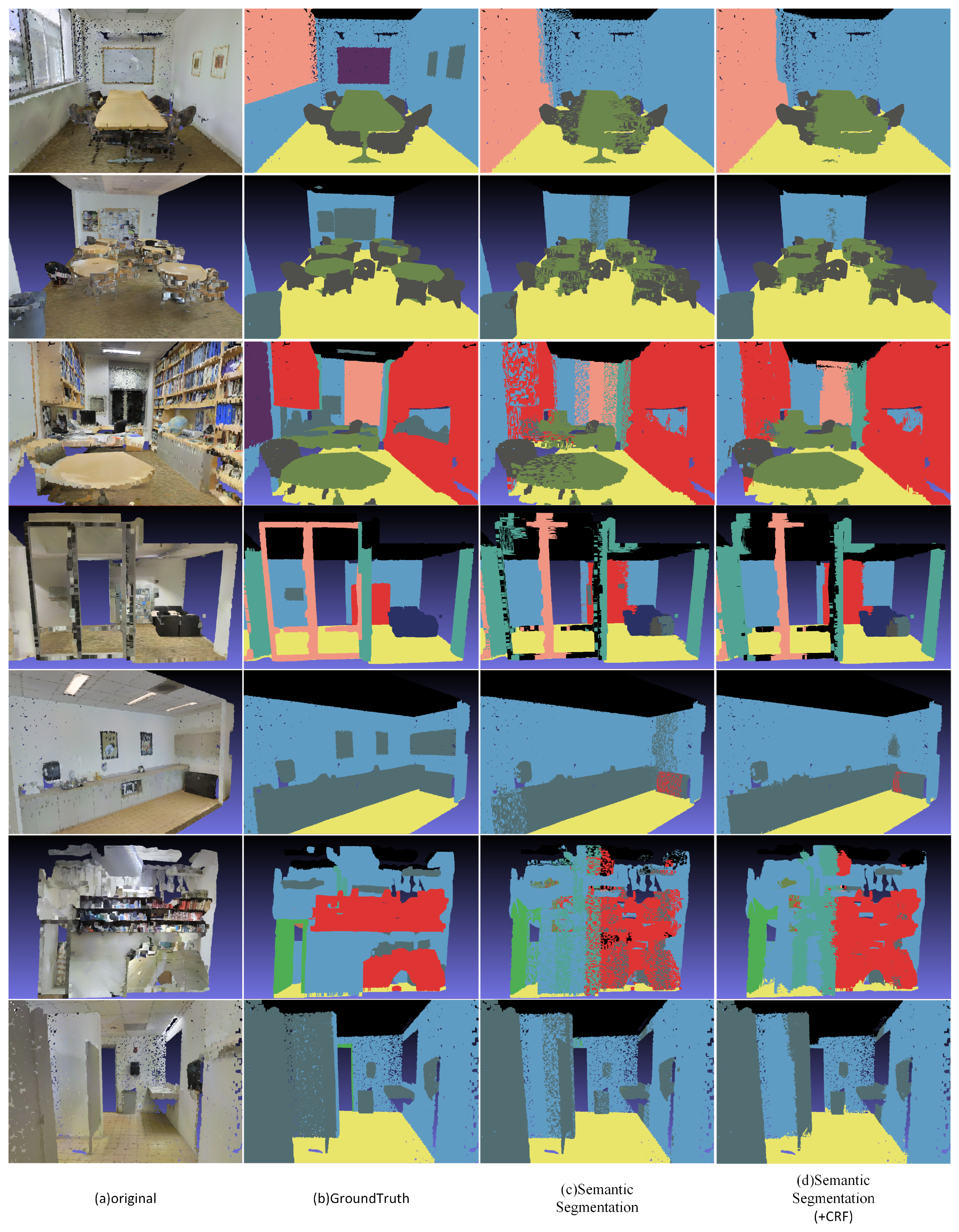
4.3. Qualitative Evalution and Comparison
5. Conclusions
Author Contributions
Funding
Institutional Review Board Statement
Informed Consent Statement
Data Availability Statement
Conflicts of Interest
References
- Qi, C.R.; Su, H.; Mo, K.; Guibas, L.J. Pointnet: Deep learning on point sets for 3D classification and segmentation. In Proceedings of the IEEE Conference on Computer Vision and Pattern Recognition, Honolulu, HI, USA, 21–26 July 2017. [Google Scholar]
- Qi, C.R.; Yi, L.; Su, H.; Guibas, L.J. Pointnet++: Deep hierarchical feature learning on point sets in a metric space. In Advances in Neural Information Processing Systems; Guyon, I., Luxburg, U.V., Bengio, S., Wallach, H., Fergus, R., Vishwanathan, S., Garnett, R., Eds.; Curran Associates, Inc.: Red Hook, NY, USA, 2017; pp. 5099–5108. [Google Scholar]
- Qi, C.R.; Liu, W.; Wu, C.; Su, H.; Guibas, L.J. Frustum pointnets for 3d object detection from rgb-d data. In Proceedings of the IEEE/CVF Conference on Computer Vision and Pattern Recognition, Salt Lake City, UT, USA, 18–22 June 2018; pp. 918–927. [Google Scholar]
- Qi, C.R.; Su, H.; Niessner, M.; Dai, A.; Yan, M.; Guibas, L.J. Volumetric and multi-view CNNs for object classification on 3D data. arXiv 2016, arXiv:1604.03265. [Google Scholar]
- Yi, L.; Su, H.; Guo, X.; Guibas, L. Syncspeccnn: Synchronized spectral cnn for 3D shape segmentation. In Proceedings of the IEEE Conference on Computer Vision and Pattern Recognition (CVPR), Honolulu, HI, USA, 21–26 July 2017; pp. 6584–6592. [Google Scholar]
- Hwang, S.S.; Kim, H.D.; Jang, T.Y.; Yoo, J.; Kim, S.; Paeng, K.; Kim, S.D. Image-based object reconstruction using run-length representation. Signal Process. Image Commun. 2017, 51, 1–12. [Google Scholar] [CrossRef]
- Han, X.F.; Laga, H.; Bennamoun, M. Image-based 3D object reconstruction: State-of-the-art and trends in the deep learning era. IEEE Trans. Pattern Anal. Mach. Intell. 2019, 43, 1578–1604. [Google Scholar] [CrossRef] [PubMed] [Green Version]
- Huang, Q.; Wang, F.; Guibas, L. Functional map networks for analyzing and exploring large shape collections. ACM Trans. Graph. 2014, 33, 1–11. [Google Scholar] [CrossRef]
- Qi, C.R.; Su, H.; Niessner, M.; Dai, A.; Yan, M.; Guibas, L.J. Volumetric and multi-view cnns for object classification on 3D data. In Proceedings of the IEEE Conference on Computer Vision and Pattern Recognition (CVPR), Las Vegas, NV, USA, 27–30 June 2016; pp. 5648–5656. [Google Scholar]
- Wu, Z.; S, S.; A, K.; Yu, F.; Zhang, L.; Tang, X.; Xiao, J. 3d shapenets: A deep representation for volumetric shapes. In Proceedings of the IEEE Conference on Computer Vision and Pattern Recognition (CVPR), Boston, MA, USA, 7–12 June 2015; pp. 1912–1920. [Google Scholar]
- Huang, J.; You, S. Vehicle detection in urban point clouds with orthogonal-view convolutional neural network. In Proceedings of the IEEE International Conference on Image Processing (ICIP), Phoenix, AZ, USA, 25–28 September 2016; pp. 2593–2597. [Google Scholar]
- Engelcke, M.; Rao, D.; Wang, D.Z.; Tong, C.H.; Posner, I. Vote3deep: Fast object detection in 3d point clouds using efficient convolutional neural networks. In Proceedings of the IEEE International Conference on Robotics and Automation (ICRA), Singapore, 29 May–3 June 2017; pp. 1355–1361. [Google Scholar]
- Li, Y.; Pirk, S.; Su, H.; Qi, C.R.; Guibas, L.J. Fpnn: Field probing neural networks for 3D data. In Advances in Neural Information Processing Systems 29; Lee, D.D., Sugiyama, M., Luxburg, U.V., Guyon, I., Garnett, R., Eds.; Curran Associates, Inc.: Red Hook, NY, USA, 2016; pp. 307–315. [Google Scholar]
- Tchapmi, L.; Choy, C.; Armeni, I.; Gwak, J.; Savarese, S. Segcloud: Semantic segmentation of 3D point clouds. In Proceedings of the International Conference on 3D Vision (3DV), Qingdao, China, 10–12 October 2017; pp. 537–547. [Google Scholar]
- Wang, P.S.; Sun, C.Y.; Liu, Y.; Tong, X. Adaptive O-CNN: A patch-based deep representation of 3D shapes. ACM Trans. Graph. 2019, 37, 1–11. [Google Scholar] [CrossRef] [Green Version]
- Tatarchenko, M.; Dosovitskiy, A.; Brox, T. Octree generating networks: Efficient convolutional architectures for highresolution 3d outputs. In Proceedings of the IEEE International Conference on Computer Vision (ICCV), Venice, Italy, 22–29 October 2017; pp. 2107–2115. [Google Scholar]
- Masci, J.; Boscaini, D.; Bronstein, M.M.; Vandergheynst, P. Geodesic convolutional neural networks on riemannian manifolds. In Proceedings of the IEEE International Conference on Computer Vision Workshop (ICCVW), Santiago, Chile, 7–13 December 2015; pp. 832–840. [Google Scholar]
- Groh, F.; Wieschollek, P.; Lensch, H.P.A. Flexconvolution (deep learning beyond grid-worlds). arXiv 2018, arXiv:1803.07289. [Google Scholar]
- Klokov, R.; Lempitsky, V. Escape from cells: Deep kdnetworks for the recognition of 3d point cloud models. In Proceedings of the IEEE International Conference on Computer Vision (ICCV), Venice, Italy, 22–29 October 2017; pp. 863–872. [Google Scholar]
- Rao, Y.; Fan, B.; Wang, Q.; Pu, J.; Luo, X.; Jin, R. Extreme feature regions detection and accurate quality assessment for point-cloud 3D reconstruction. IEEE Access 2019, 7, 37757–37769. [Google Scholar] [CrossRef]
- Nguyen, D.T.; Hua, B.; Yu, L.; Yeung, S. A robust 3D-2D interactive tool for scene segmentation and annotation. IEEE Trans. Vis. Comput. Graph. 2018, 24, 3005–3018. [Google Scholar] [CrossRef] [PubMed] [Green Version]
- Wang, T.C.; Yang, T.; Danelljan, M.; Khan, F.S.; Zhang, X.Y.; Sun, J. Learning human-object interaction detection using interaction points. In Proceedings of the IEEE/CVF Conference on Computer Vision and Pattern Recognition, CVPR 2020, Seattle, WA, USA, 13–19 June 2020; pp. 4115–4124. [Google Scholar]
- Wen, X.; Li, T.Y.; Han, Z.Z.; Liu, Y.S. Point cloud completion by skip-attention network with hierarchical folding. In Proceedings of the IEEE/CVF Conference on Computer Vision and Pattern Recognition, CVPR 2020, Seattle, WA, USA, 13–19 June 2020; pp. 1936–1945. [Google Scholar]
- Li, L.; Zhu, S.Y.; Fu, H.B.; Tan, P.; Tai, C.L. End-to-end learning local multi-view descriptors for 3D point clouds. In Proceedings of the IEEE/CVFConference on Computer Vision and Pattern Recognition, CVPR 2020, Seattle, WA, USA, 13–19 June 2020; pp. 1916–1925. [Google Scholar]
- Ye, X.; Li, J.; Huang, H.; Du, L.; Zhang, X. 3d recurrent neural networks with context fusion for point cloud semantic segmentation. In Proceedings of the European Conference on Computer Vision (ECCV), Munich, Germany, 8–14 September 2018. [Google Scholar]
- Landrieu, L.; Boussaha, M. Point cloud oversegmentation with graph-structured deep metric learning. In Proceedings of the IEEE/CVF Conference on Computer Vision and Pattern Recognition (CVPR), Long Beach, CA, USA, 16–20 June 2019; pp. 7432–7441. [Google Scholar]
- Landrieu, L.; Simonovsky, M. Large-scale Point cloud semantic segmentation with superpoint graphs. In Proceedings of the IEEE Conference on Computer Vision and Pattern Recognition (CVPR), Salt Lake City, UT, USA, 18–23 June 2018; pp. 4558–4567. [Google Scholar]
- Zhang, L.; Zhu, Z. Unsupervised feature learning for point cloud understanding by contrasting and clustering using graph convolutional neural networks. In Proceedings of the International Conference on 3D Vision (3DV), Quebec City, QC, Canada, 16–19 September 2019; pp. 395–404. [Google Scholar]
- Shi, W.; Rajkumar, R. Point-GNN: Graph Neural Network for 3D Object Detection in a Point Cloud. In Proceedings of the IEEE/CVF Conference on Computer Vision and Pattern Recognition, CVPR 2020, Seattle, WA, USA, 13–19 June 2020; pp. 1708–1716. [Google Scholar]
- Xie, Z.; Chen, J.; Peng, B. Point clouds learning with attention-based graph convolution networks. arXiv 2019, arXiv:1905.13445. [Google Scholar]
- Wu, W.; Zhang, Y.; Wang, D.; Lei, Y. SK-Net: Deep learning on point cloud via end-to-end discovery of spatial keypoints. In Proceedings of the Thirty-Fourth AAAI Conference on Artificial Intelligence, AAAI 2020, New York, NY, USA, 7–12 February 2020; pp. 6422–6429. [Google Scholar]
- Biasutti, P.; Bugeau, A.; Aujol, J.; BréDif, M. Riu-net: Embarrassingly simple semantic segmentation of 3d lidar point cloud. arXiv 2019, arXiv:1905.08748. [Google Scholar]
- Hu, Q.; Yang, B.; Xie, L.; Rosa, S.; Guo, Y.; Wang, Z.; Trigoni, N.; Markham, A. RandLA-Net: Efficient semantic segmentation of large-scale point clouds. arXiv 2019, arXiv:1911.11236. [Google Scholar]
- Yan, X.; Zheng, C.; Li, Z.; Wang, S.; Cui, S. Pointasnl: Robust point clouds processing using nonlocal neural networks with adaptive sampling. arXiv 2020, arXiv:2003.00492. [Google Scholar]
- Pham, Q.; Hua, B.; Nguyen, T.; Yeung, S. Real-time progressive 3D semantic segmentation for indoor scenes. In Proceedings of the IEEE Winter Conference on Applications of Computer Vision (WACV), Waikoloa, HI, USA, 7–11 January 2019; pp. 1089–1098. [Google Scholar]
- Rao, Y.; Zhang, M.; Cheng, Z.; Xue, J.; Pu, J.; Wang, Z. Fast 3D point cloud segmentation using deep neural network. In Proceedings of the IEEE International Conference on Internet of Things and Intelligent Applications (ITIA2020), Zhengjiang, China, 27–29 November 2020. [Google Scholar]
- Wang, X.; Liu, S.; Shen, X.; Shen, C.; Jia, J. Associatively segmenting instances and semantics in point clouds. In Proceedings of the IEEE/CVF Conference on Computer Vision and Pattern Recognition (CVPR), Long Beach, CA, USA, 15–20 June 2019; pp. 4091–4100. [Google Scholar]
- Armeni, I.; Sener, O.; Zamir, A.R.; Jiang, H.; Brilakis, I.; Fischer, M.; Savarese, S. 3D semantic parsing of large-scale indoor spaces. In Proceedings of the IEEE Conference on Computer Vision and Pattern Recognition (CVPR), Las Vegas, NV, USA, 27–30 June 2016; pp. 1534–1543. [Google Scholar]
- Hua, B.; Tran, M.; Yeung, S. Pointwise convolutional neural networks. In Proceedings of the IEEE/CVF Conference on Computer Vision and Pattern Recognition, Salt Lake City, UT, USA, 18–22 June 2018; pp. 984–993. [Google Scholar]


| Scene (Area5) | Original Projection (PN) | Election Projection (PN) | Compression Ratio (%) |
|---|---|---|---|
| conferenceRoom1 | 1,047,554 | 118,784 | 11.34 |
| lobby1 | 1,223,236 | 131,072 | 10.72 |
| office10 | 752,349 | 90,112 | 11.98 |
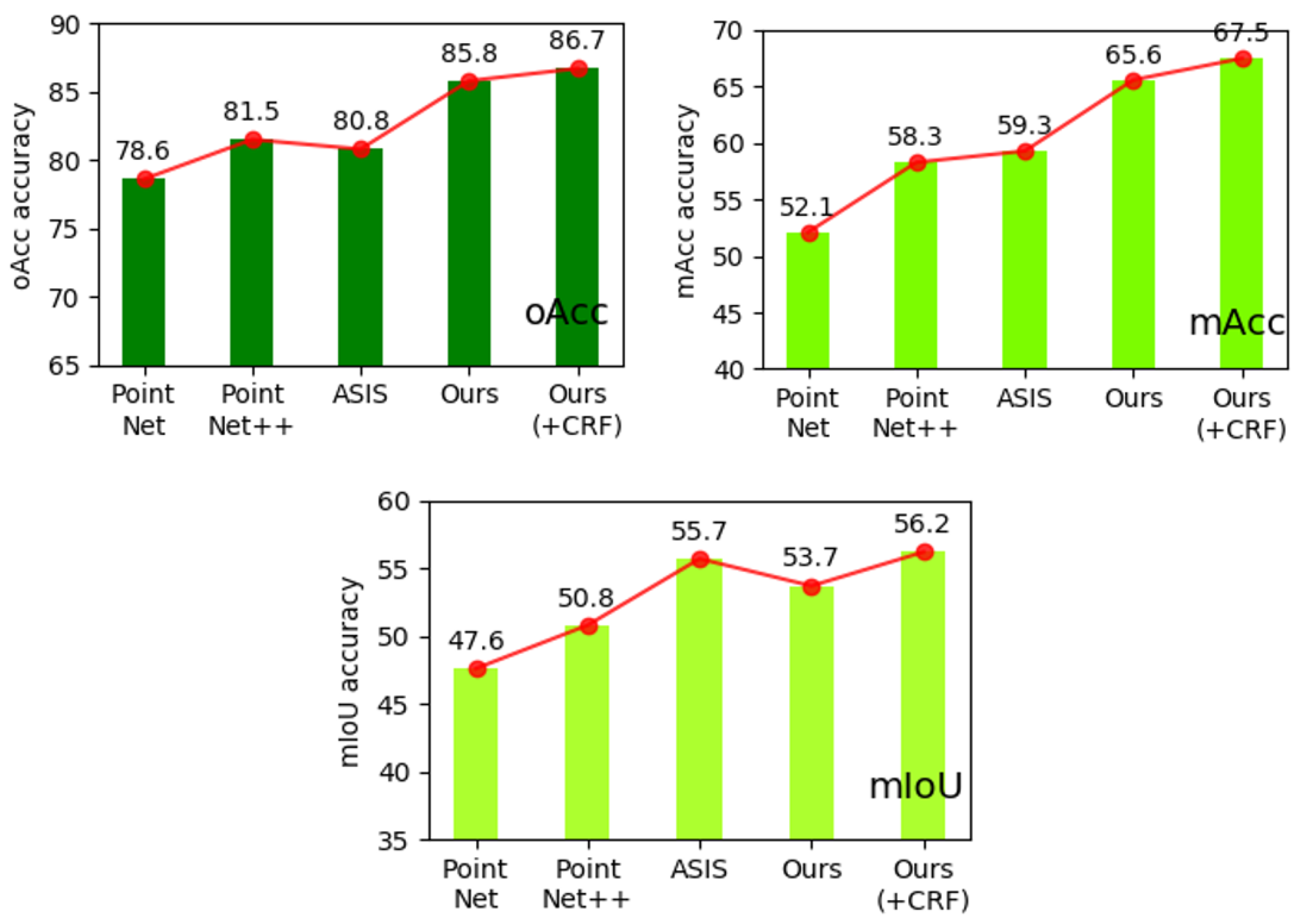
| Method | mIoU | mAcc | mRecall |
|---|---|---|---|
| PointNet [1] | 47.6 | 52.1 | - |
| PointNet++ [2] | 50.8 | 58.3 | - |
| ASIS [37] | 55.7 | 59.3 | - |
| Ours | 53.7 | 65.6 | 0.338 |
| Ours (+CRF) | 56.2 | 67.5 | 0.372 |
| Method | oAcc | Ceiling | Floor | Wall | Window | Door | Table | Chair | Sofa | Bookcase | Board | Clutter |
|---|---|---|---|---|---|---|---|---|---|---|---|---|
| PointNet [1] | 78.6 | 88.8 | 97.3 | 69.8 | 46.3 | 10.8 | 52.6 | 58.9 | 40.3 | 5.9 | 26.4 | 33.2 |
| Pointwise [39] | 81.5 | 97.9 | 99.3 | 92.7 | 49.6 | 50.6 | 74.1 | 58.2 | 0 | 39.3 | 0 | 61.1 |
| SEGCloud [14] | 80.8 | 90.1 | 96.1 | 69.9 | 38.4 | 23.1 | 75.9 | 70.4 | 58.4 | 40.9 | 13 | 41.6 |
| Ours | 85.8 | 96.5 | 99.2 | 86.5 | 82.4 | 57.3 | 81.1 | 65.3 | 67.9 | 74.3 | 16.3 | 55.8 |
| Ours(+CRF) | 86.7 | 97.5 | 99.3 | 86.2 | 84.8 | 59.0 | 83.7 | 65.7 | 74.7 | 78.1 | 17.2 | 53.8 |
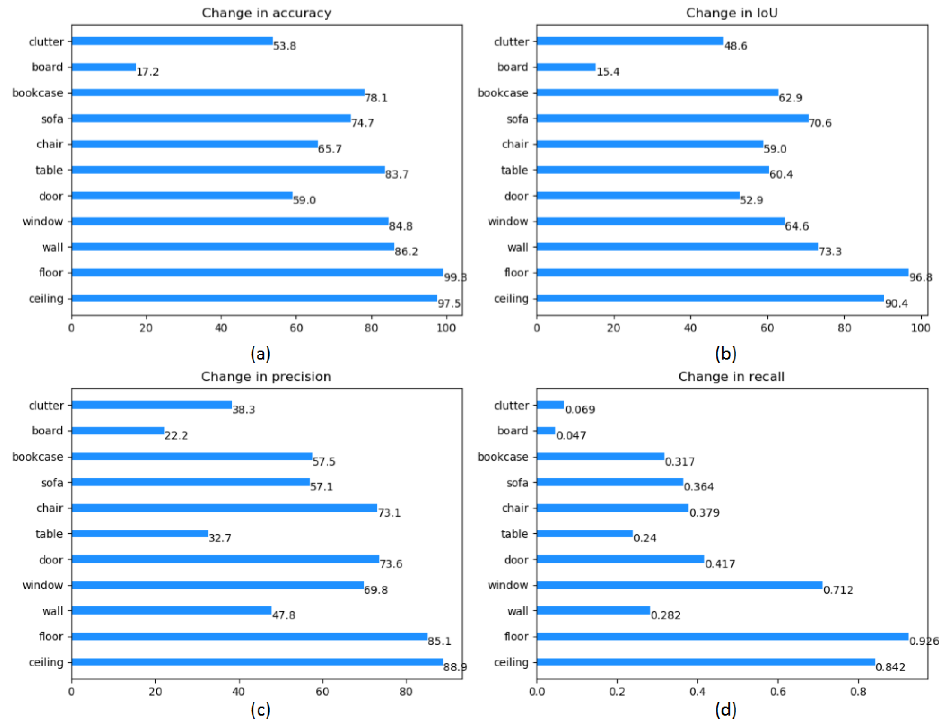
| Ceiling | Floor | Wall | Window | Door | Table | Chair | Sofa | Bookcase | Board | Clutter | |
|---|---|---|---|---|---|---|---|---|---|---|---|
| CA | 97.5 | 99.3 | 86.2 | 84.8 | 59.0 | 83.7 | 65.7 | 74.7 | 78.1 | 17.2 | 53.8 |
| CIoU | 90.4 | 96.8 | 73.3 | 64.6 | 52.9 | 60.4 | 59.0 | 70.6 | 62.9 | 15.4 | 48.6 |
| CP | 88.9 | 85.1 | 47.8 | 69.8 | 73.6 | 32.7 | 73.1 | 57.1 | 57.5 | 22.2 | 38.3 |
| CR | 0.842 | 0.926 | 0.282 | 0.712 | 0.417 | 0.240 | 0.379 | 0.364 | 0.317 | 0.047 | 0.069 |
Publisher’s Note: MDPI stays neutral with regard to jurisdictional claims in published maps and institutional affiliations. |
© 2021 by the authors. Licensee MDPI, Basel, Switzerland. This article is an open access article distributed under the terms and conditions of the Creative Commons Attribution (CC BY) license (https://creativecommons.org/licenses/by/4.0/).
Share and Cite
Rao, Y.; Zhang, M.; Cheng, Z.; Xue, J.; Pu, J.; Wang, Z. Semantic Point Cloud Segmentation Using Fast Deep Neural Network and DCRF. Sensors 2021, 21, 2731. https://doi.org/10.3390/s21082731
Rao Y, Zhang M, Cheng Z, Xue J, Pu J, Wang Z. Semantic Point Cloud Segmentation Using Fast Deep Neural Network and DCRF. Sensors. 2021; 21(8):2731. https://doi.org/10.3390/s21082731
Chicago/Turabian StyleRao, Yunbo, Menghan Zhang, Zhanglin Cheng, Junmin Xue, Jiansu Pu, and Zairong Wang. 2021. "Semantic Point Cloud Segmentation Using Fast Deep Neural Network and DCRF" Sensors 21, no. 8: 2731. https://doi.org/10.3390/s21082731