
Applying Machine Learning Technologies Based on Historical Activity Features for Multi-Resident Activity Recognition


Abstract
:1. Introduction
2. Related Work
3. Problem Definition
4. The Proposed Methods
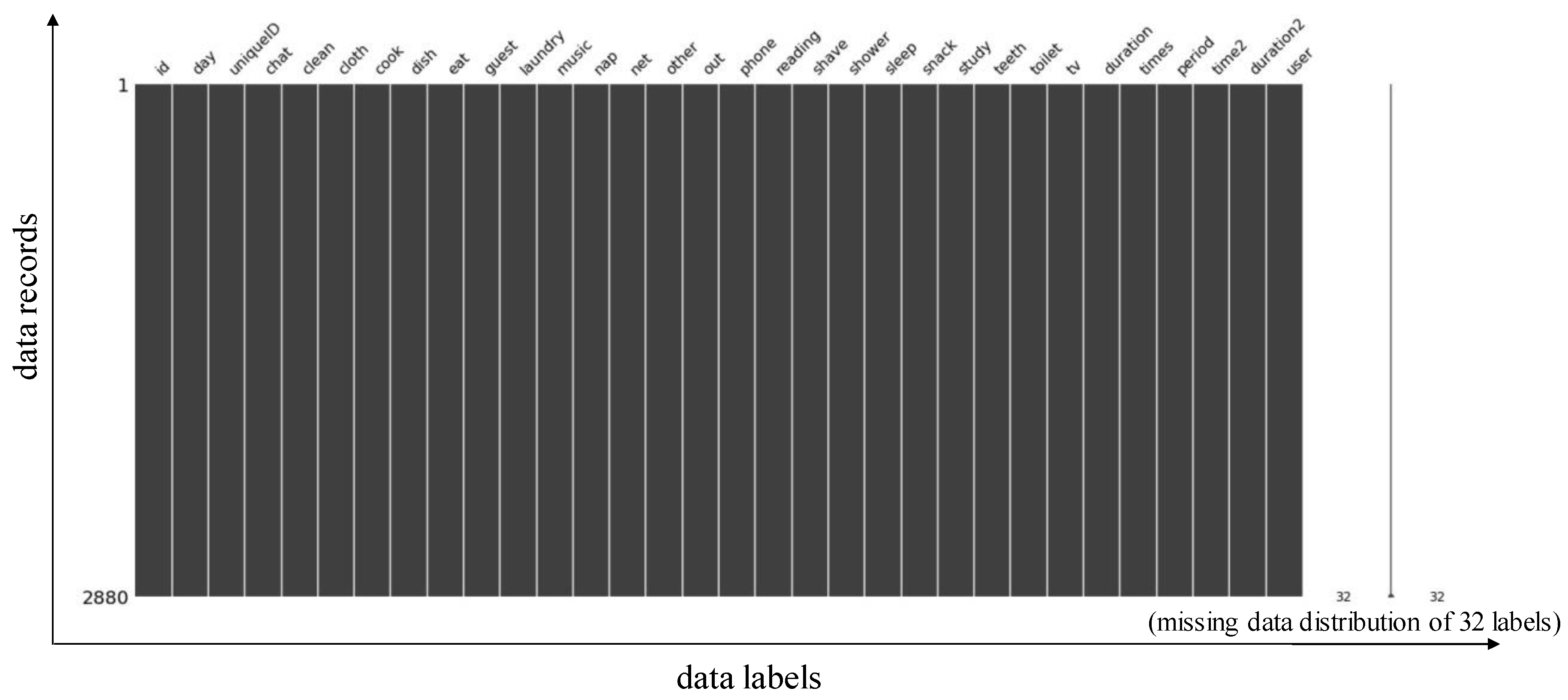
4.1. Data Collection and Preprocessing
- Data Preprocessing
- Standardization of Features
- Feature Selection
4.2. Machine Learning Methods
- Support Vector Machine (SVM)
- K-Nearest Neighbor (KNN)
- (1)
- Calculate the distance between the test object and all objects in the training set, where the most commonly used is Euclidean distance [30].
- (2)
- Find the closest K objects in the distance calculated in the previous step as neighbors of the test object.
- (3)
- Find the object with the highest frequency among the K objects, and its category is the category to which the test object belongs.
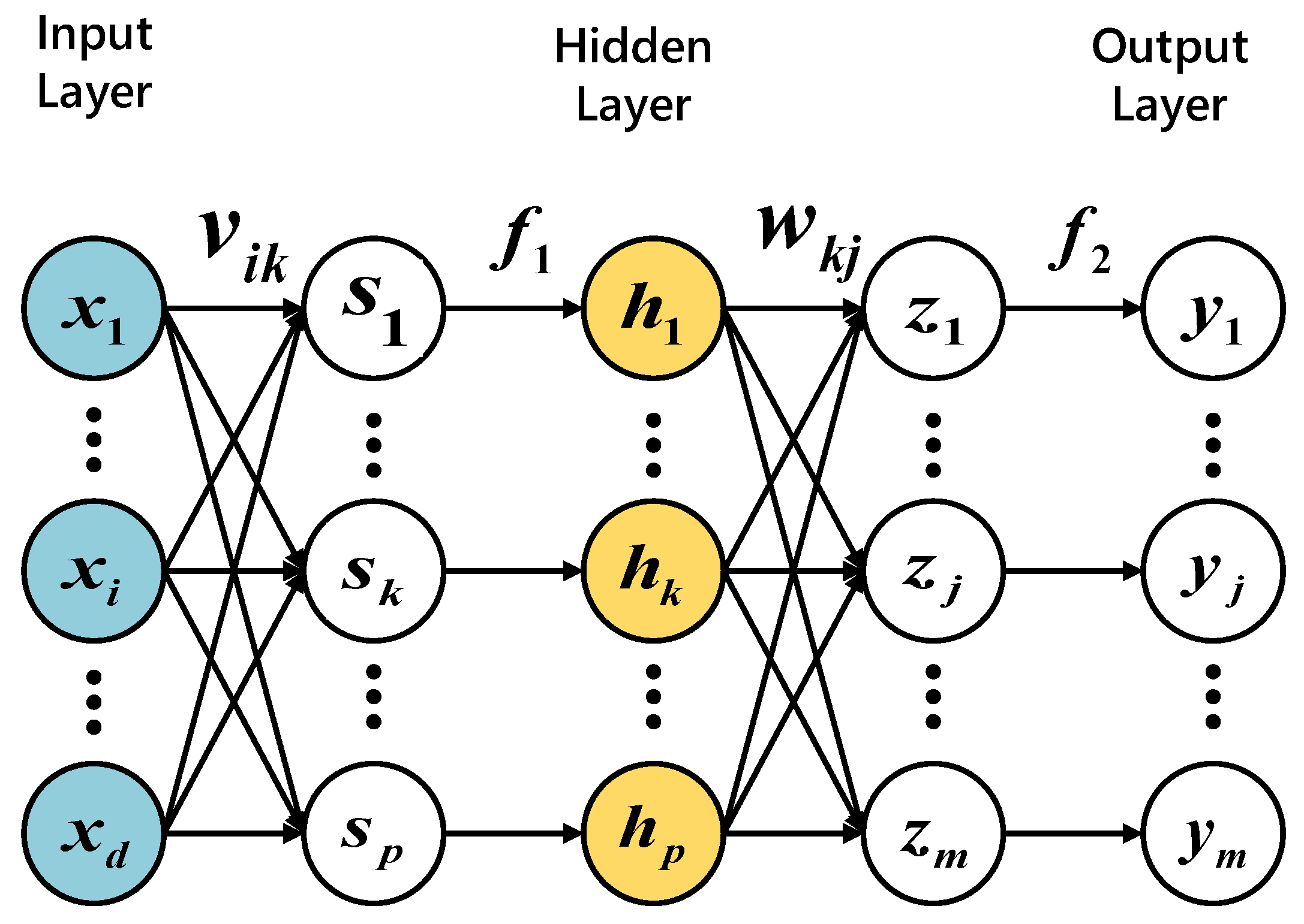
- Multilayer Perceptron (MLP)
- Random Forest (RF)
- J48 Decision Tree (J48DT)
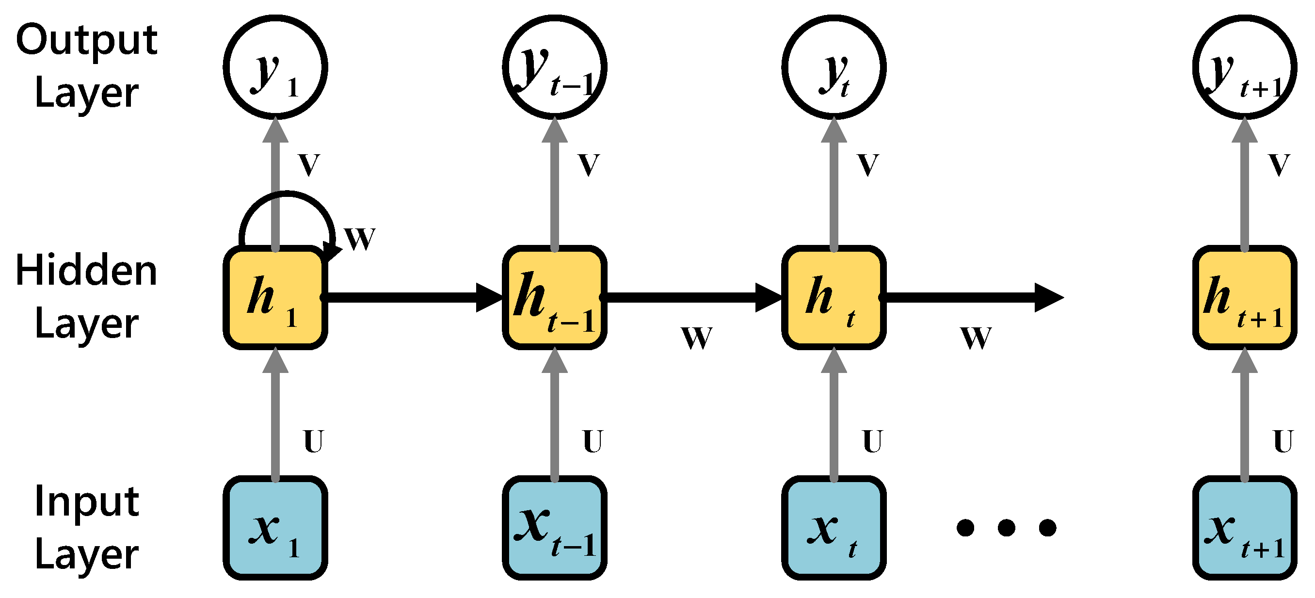
- Recurrent Neural Network (RNN)
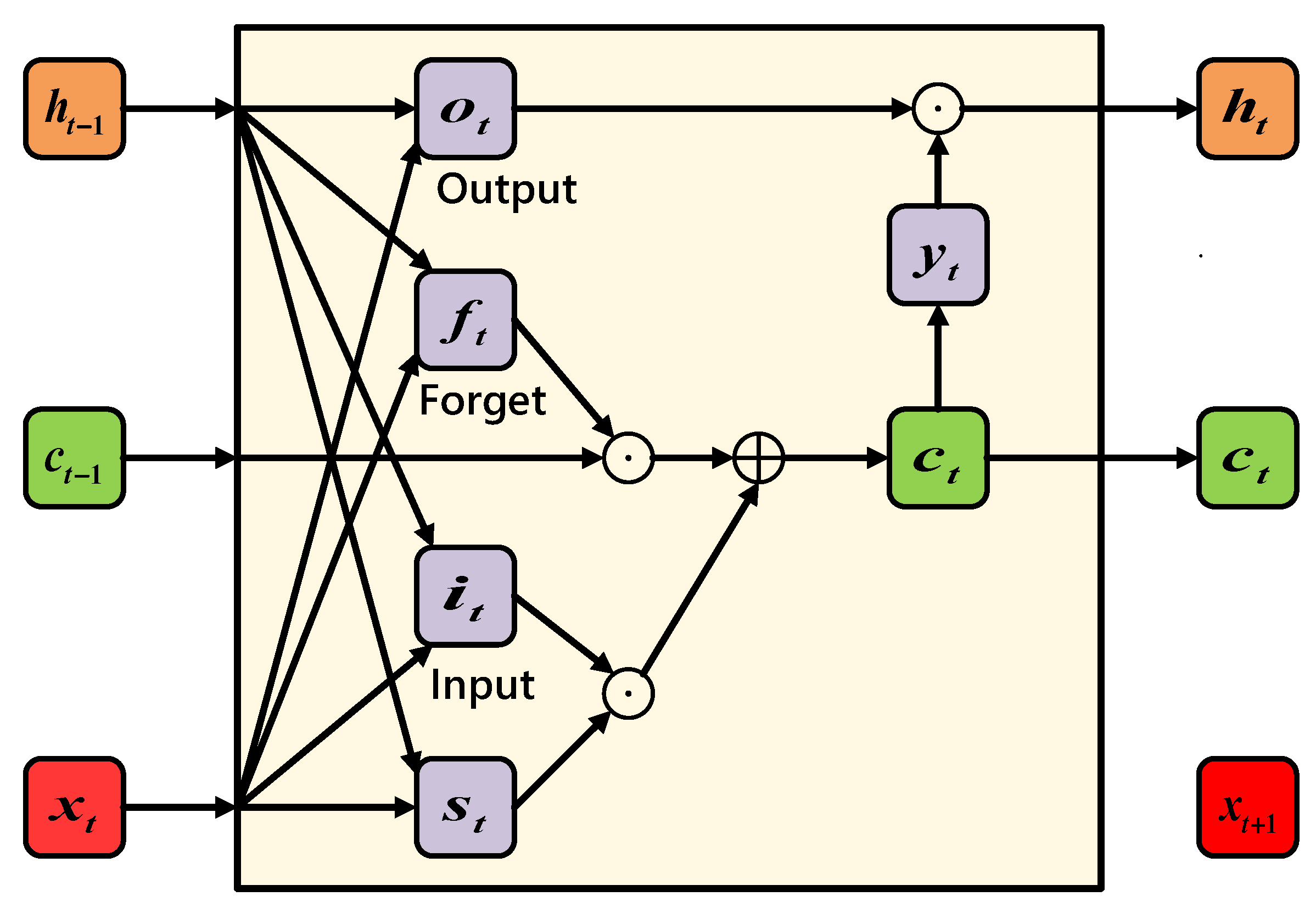
- Long Short-Term Memory (LSTM)
5. Performance Evaluation
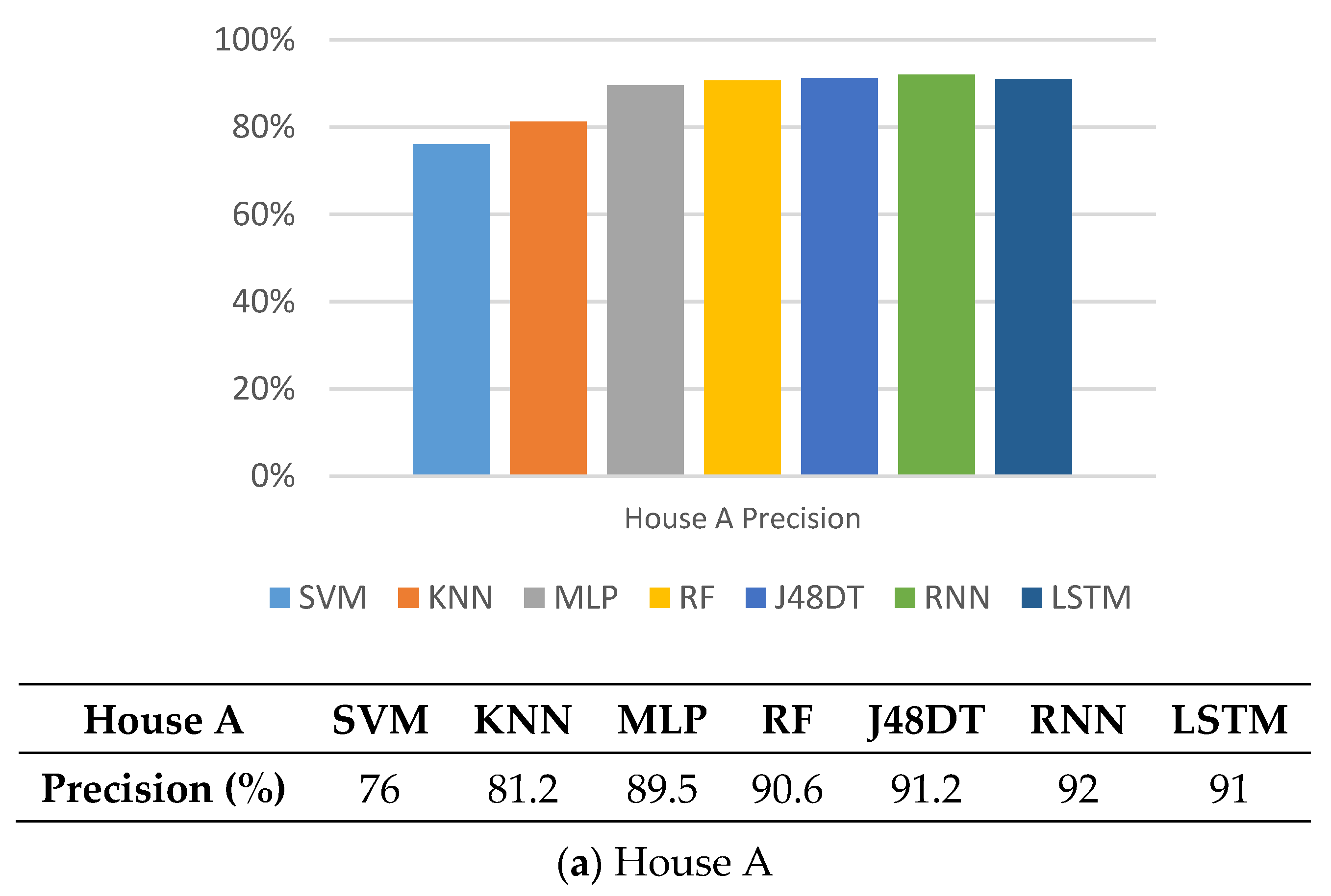
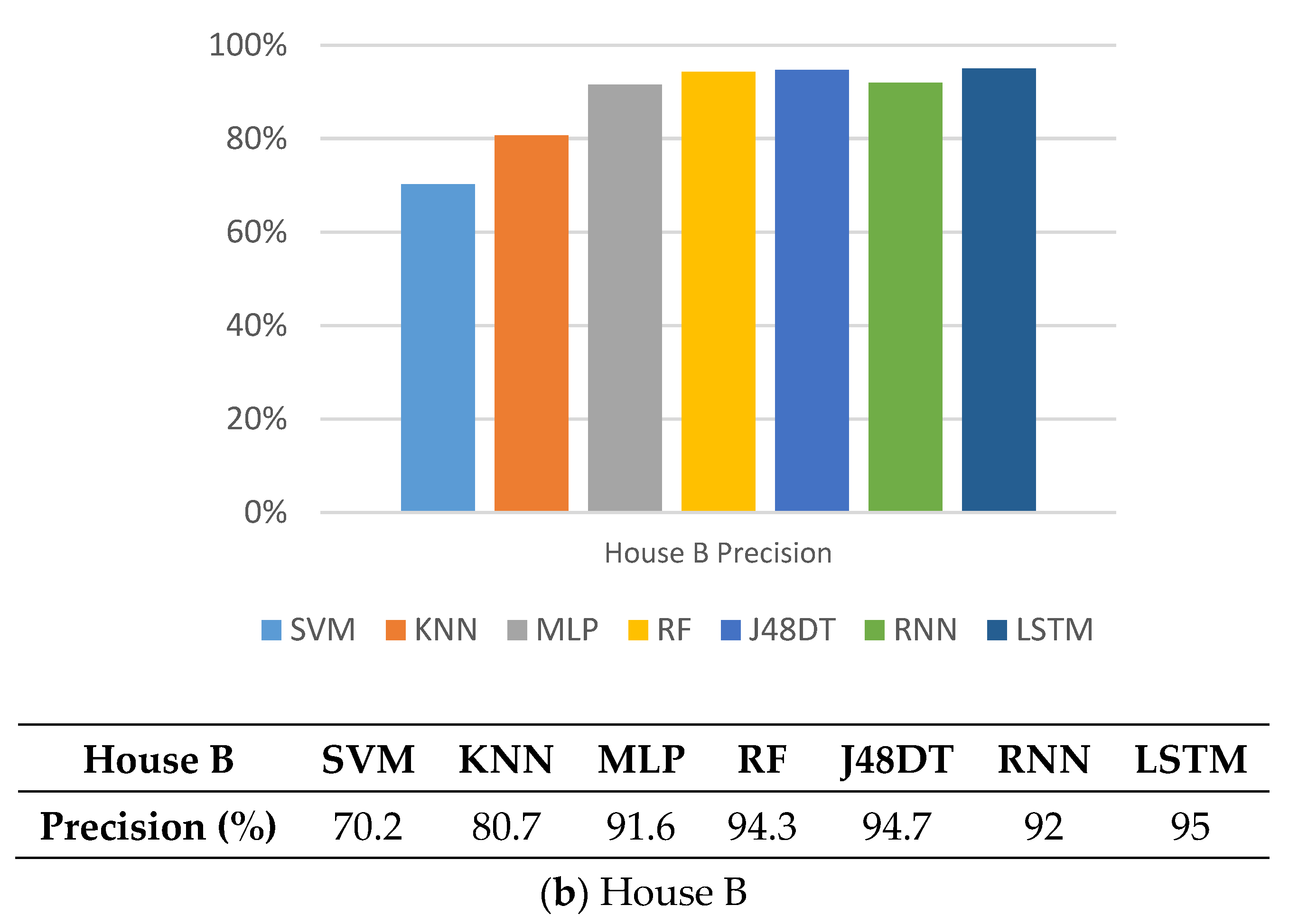
5.1. Precision
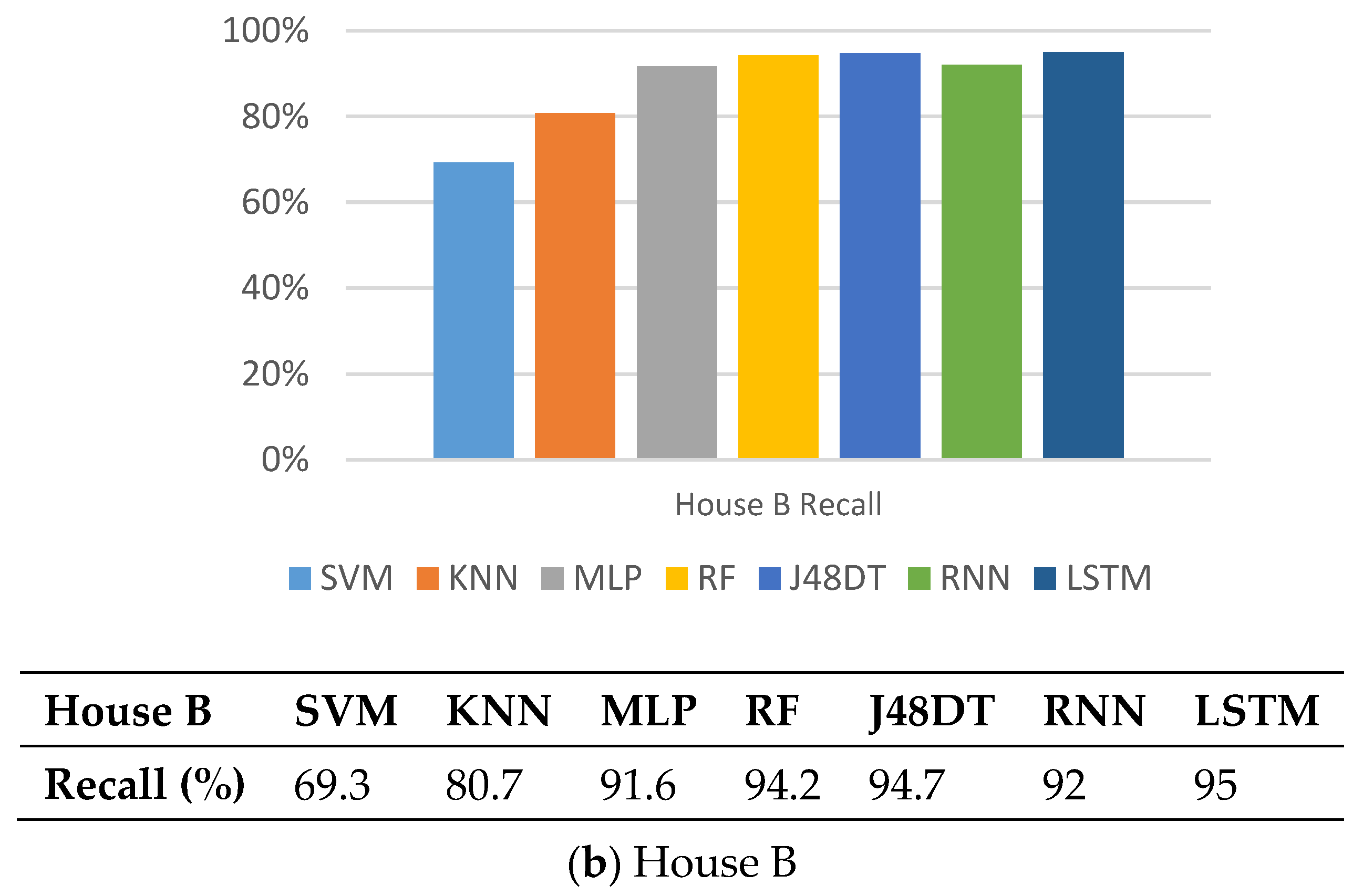
5.2. Recall
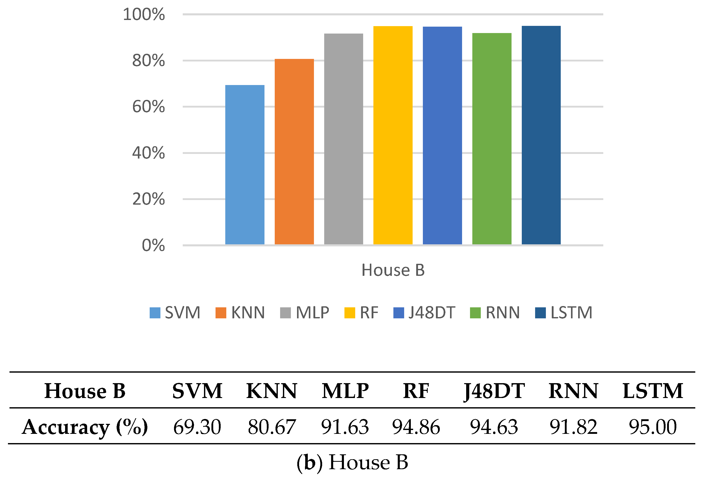
5.3. Accuracy
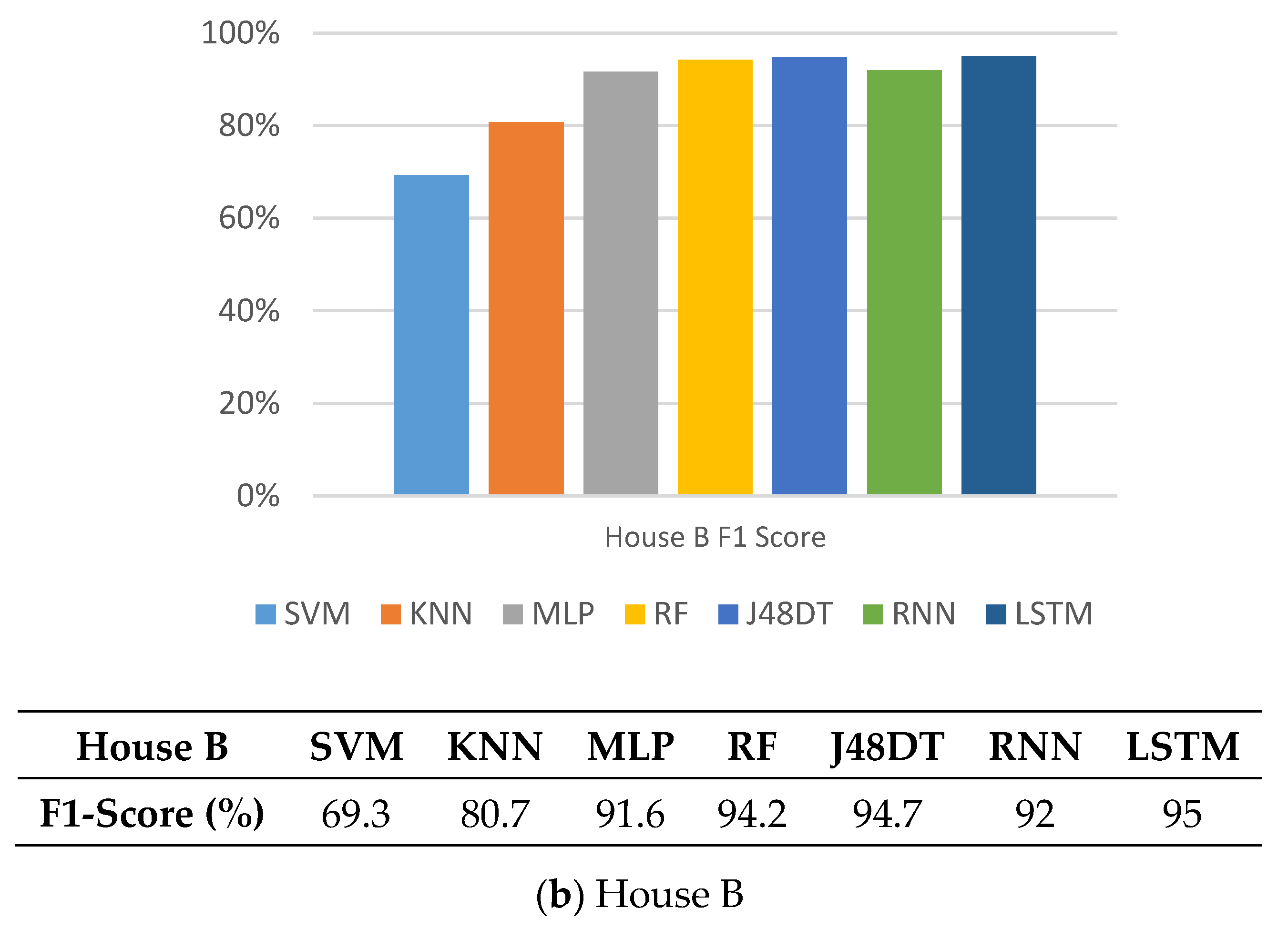
5.4. F1-Score
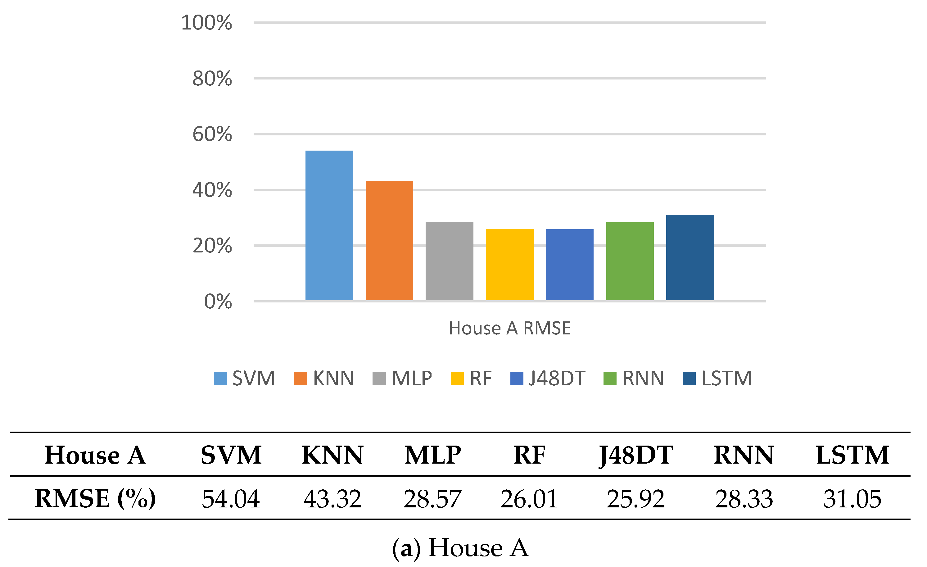
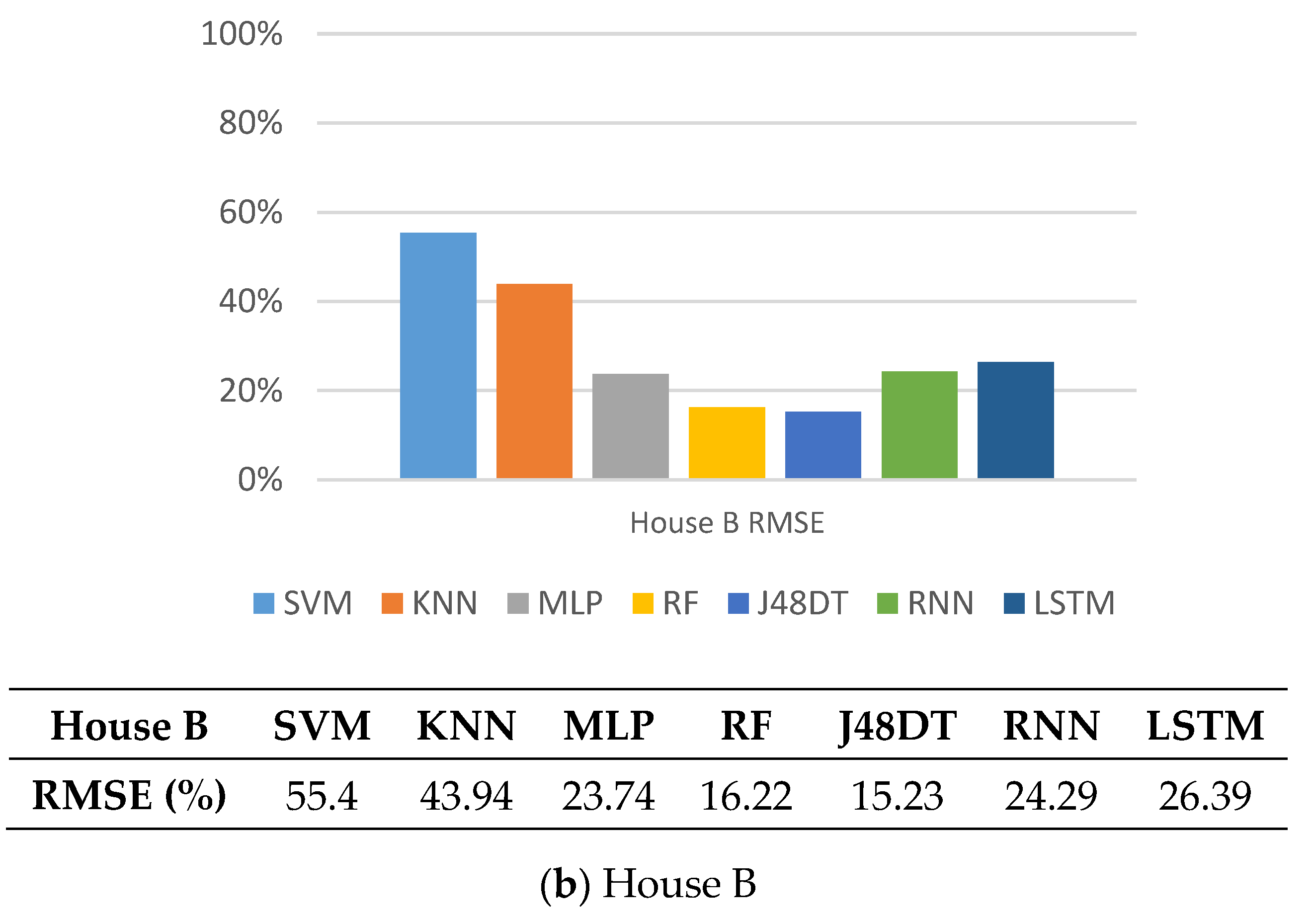
5.5. RMSE
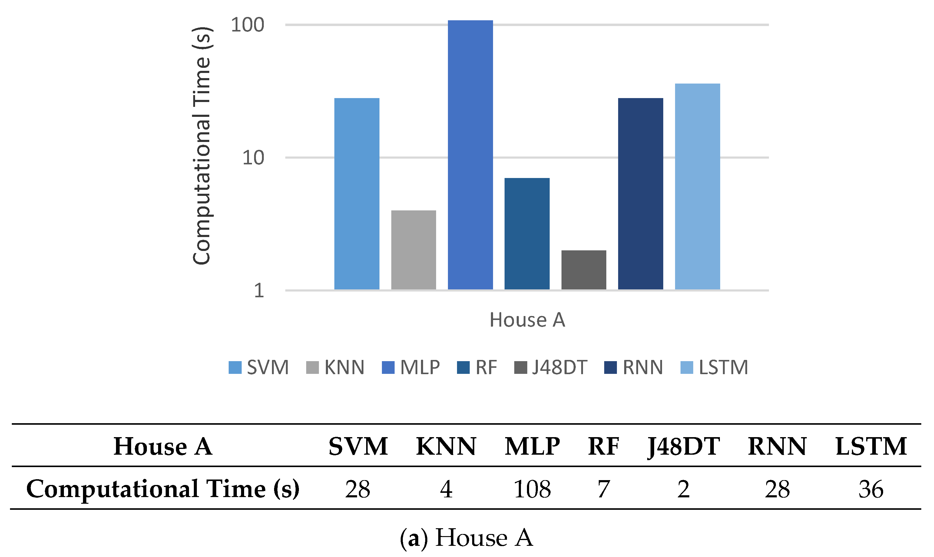
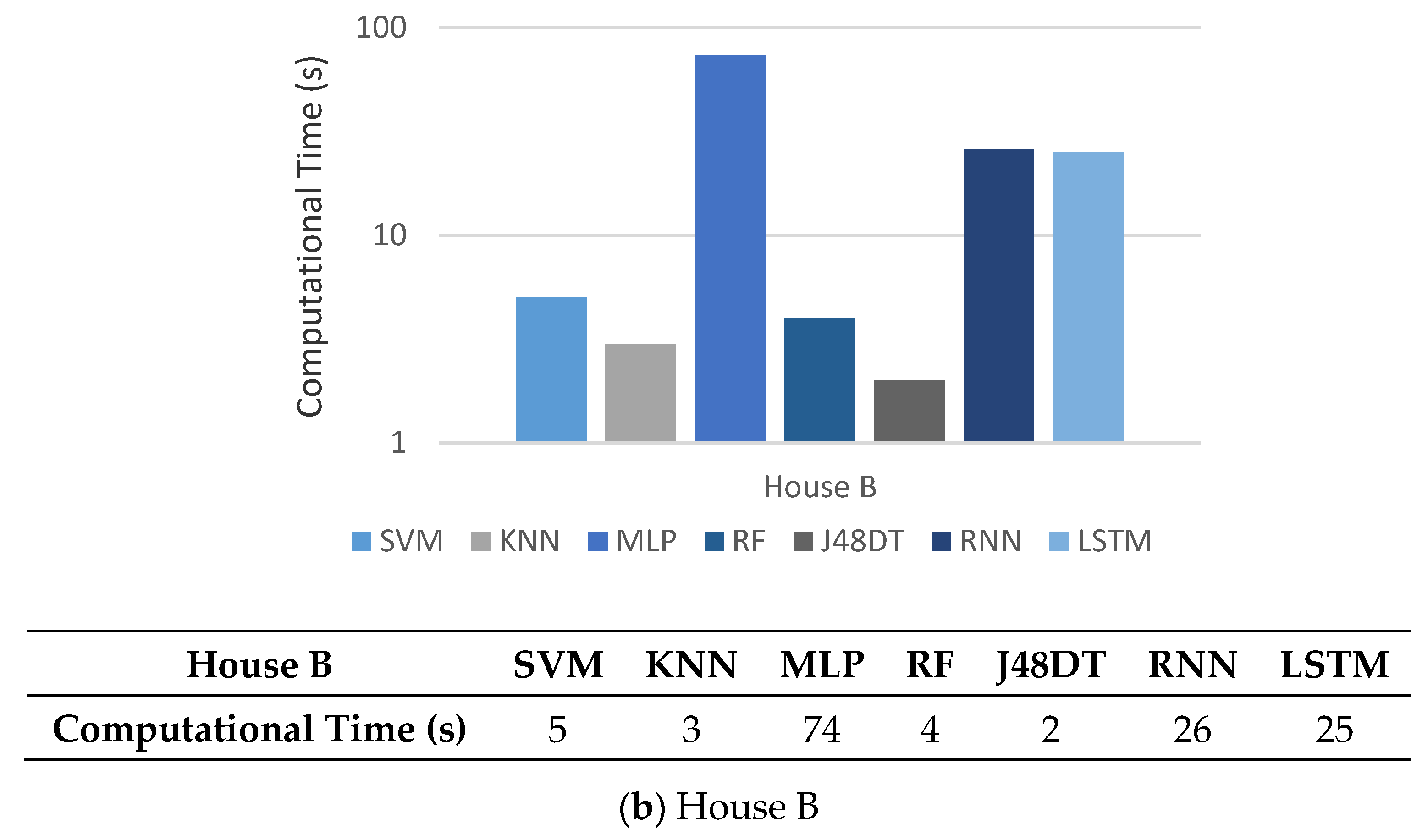
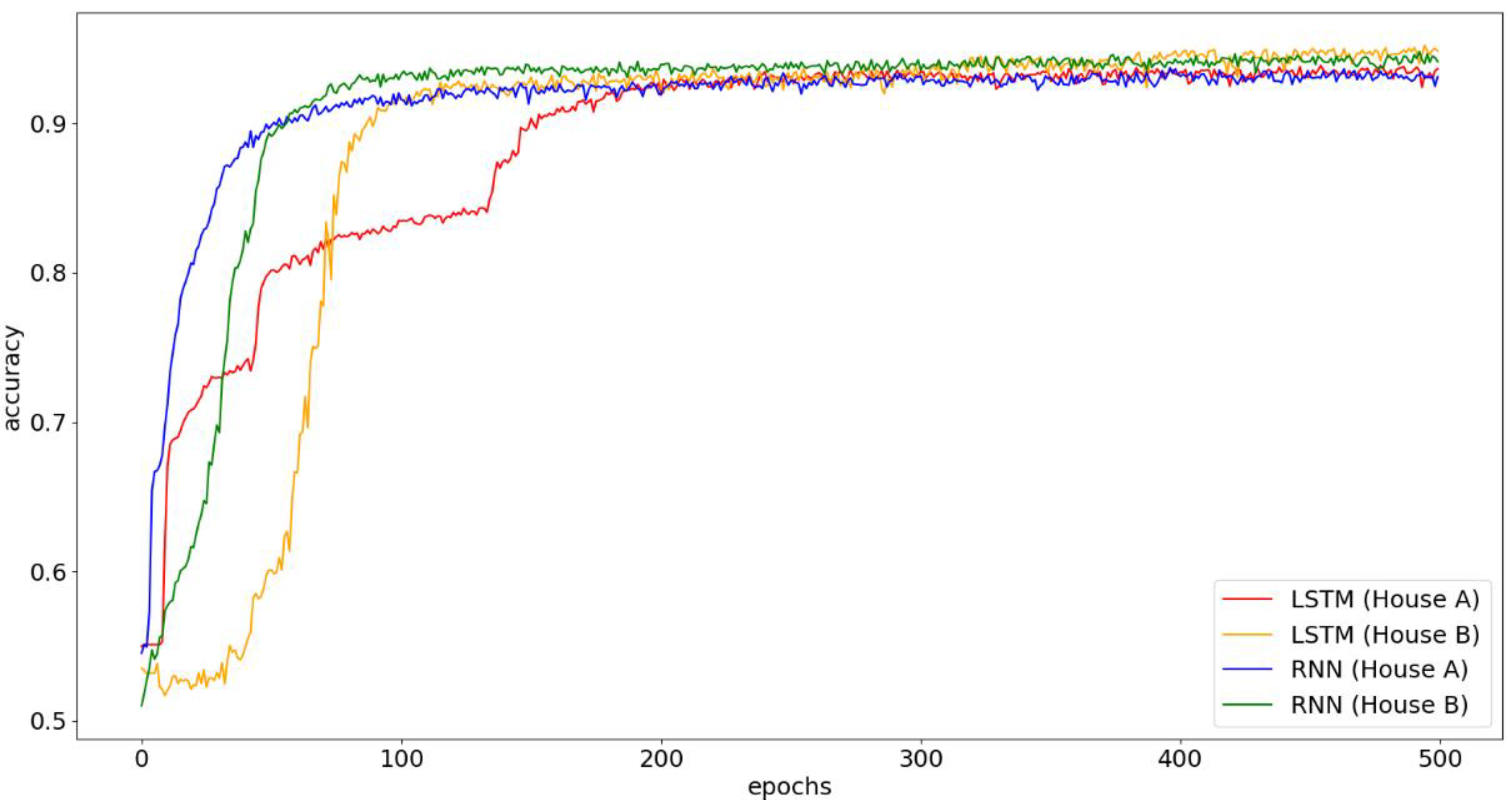
5.6. Computational Complexity
5.7. Observations
5.8. Discussions
6. Conclusions
Author Contributions
Funding
Institutional Review Board Statement
Informed Consent Statement
Data Availability Statement
Conflicts of Interest
References
- Zikria, Y.B.; KhalilAfzal, M.; Kim, S.W.; Marin, A.; Guizani, M. Deep learning for intelligent IoT: Opportunities, challenges and solutions. Comput. Commun. 2020, 164, 50–53. [Google Scholar] [CrossRef]
- Pereira, C.; Mesquita, J.; Guimarães, D.; Santos, F.; Almeida, L.; Aguiar, A. Open IoT Architecture for continuous patient monitoring in emergency wards. Electronics 2019, 8, 1074. [Google Scholar] [CrossRef] [Green Version]
- Hassan, S.R.; Ahmad, I.; Ahmad, S.; Alfaify, A.; Shafiq, M. Remote pain monitoring using fog computing for e-Healthcare: An efficient architecture. Sensors 2020, 20, 6574. [Google Scholar] [CrossRef] [PubMed]
- Sampath, P.; Packiriswamy, G.; Kumar, N.P.; Shanmuganathan, V.; Song, O.-Y.; Tariq, U.; Nawaz, R. IoT based health-Related topic recognition from emerging online health community (Med Help) using machine learning technique. Electronics 2020, 9, 1469. [Google Scholar] [CrossRef]
- Lussier, M.; Aboujaoudé, A.; Couture, M.; Moreau, M.; Laliberté, C.; Giroux, S.; Pigot, H.; Gaboury, S.; Bouchard, K.; Belchior, P.; et al. Using ambient assisted living to monitor older adults with alzheimer disease: Single-case study to validate the monitoring report. JMIR Med. Inform. 2020, 8, 1–16. [Google Scholar] [CrossRef] [PubMed]
- Wang, J.; Chen, Y.; Hao, S.; Peng, X.; Hu, L. Deep learning for sensor-based activity recognition: A survey. Pattern Recognit. Lett. 2019, 119, 3–11. [Google Scholar] [CrossRef] [Green Version]
- Hamad, R.A.; Hidalgo, A.S.; Bouguelia, M.-R.; Estevez, M.E.; Quero, J.M. Efficient activity recognition in smart homes using delayed fuzzy temporal windows on binary sensors. IEEE J. Biomed. Health Inform. 2020, 24, 387–395. [Google Scholar] [CrossRef]
- Thapa, K.; Abdullah, A.; Lamichhane, Z.M.; Yang, S.-H. A deep machine learning method for concurrent and interleaved human activity recognition. Sensors 2020, 20, 5770. [Google Scholar] [CrossRef] [PubMed]
- Kim, K.; Jalal, A.; Mahmood, M. Vision-based human activity recognition system using depth silhouettes: A smart home system for monitoring the residents. J. Electr. Eng. Technol. 2019, 14, 2567–2573. [Google Scholar] [CrossRef]
- Jeghama, I.; Khalifab, A.B.; Alouanic, I.; Mahjoub, M.A. Vision-based human action recognition: An overview and real world challenges. Forensic Sci. Int. Digit. Investig. 2020, 32, 1–17. [Google Scholar] [CrossRef]
- Du, W.; Li, A.; Zhou, P.; Niu, B.; Wu, D. Privacyeye: A privacy-preserving and computationally efficient deep learning-based mobile video analytics system. IEEE Trans. Mob. Comput. 2021, 1, 1–18. [Google Scholar] [CrossRef]
- Hu, N.; Su, S.; Tang, C.; Wang, L. Wearable-sensors based activity recognition for smart human healthcare using internet of things. Int. Wirel. Commun. Mob. Comput. 2020, 1909–1915. [Google Scholar] [CrossRef]
- Malasé, A.; Maurice, P.; Colas, F.; Charpillet, F.; Ivaldi, S. Activity recognition with multiple wearable sensors for industrial applications. In Proceedings of the the Eleventh International Conference on Advances in Computer-Human Interactions, Rome, Italy, 25–29 March 2018. [Google Scholar]
- Wang, J.; Chen, Y.; Hao, S.; Peng, X.; Hu, L. Deep human activity recognition with localisation of wearable sensors. IEEE Access 2020, 8, 155060–155070. [Google Scholar]
- Wan, S.; Qi, L.; Xu, X.; Tong, C.; Gu, Z. Deep learning models for real-time human activity recognition with smartphones. Mob. Netw. Appl. 2020, 25, 743–755. [Google Scholar] [CrossRef]
- Bai, Y.; Wang, X. CARIN: Wireless CSI-based driver activity recognition under the interference of passengers. ACM Interact. Mob. Wearable Ubiquitous Technol. 2020, 4, 1–28. [Google Scholar] [CrossRef] [Green Version]
- Aging Project: Living Together with Your Friends. Available online: http://www.activageproject.eu/blog/2020/02/11/Aging-Project-Living-together-with-your-friends/ (accessed on 15 February 2021).
- Arrigoitia, M.F.; West, K. Interdependence, commitment, learning and love. The case of the United Kingdom′s first older women’s co-housing community. Ageing Soc. 2020, 1–35. [Google Scholar] [CrossRef] [Green Version]
- Dühr, S. The role of government in supporting co-housing accommodation models for older people in Germany: Towards a research agenda. Univ. S. Aust. 2020, 1–35. [Google Scholar] [CrossRef]
- Mohamed, R.; Perumal, T.; Sulaiman, M.N.; Mustapha, N.; Zainudin, M.N.S. Modeling activity recognition of multi resident using label combination of multilabel classification in smart home. AIP Conf. Proc. 2017, 1–7. [Google Scholar] [CrossRef] [Green Version]
- Rogelj, V.; Bogataj, D. Ambient assisted living technologies and environments: Literature review and research agenda. In Proceedings of the International Conference on Control, Decision and Information Technologies, Prague, Czech Republic, 29 June–2 July 2020; pp. 762–767. [Google Scholar]
- Manuel, J.G.G.; Augusto, J.C.; Stewart, J. AnAbEL: Towards empowering people living with dementia in ambient assisted living. Univers. Access Inf. Soc. 2020, 1, 1–20. [Google Scholar]
- Taylor, W.; Shah, S.A.; Dashtipour, K.; Zahid, A.; Abbasi, Q.H.; Imran, M.A. An intelligent non-invasive real-time human activity recognition system for next-generation healthcare. Sensors 2020, 20, 2653. [Google Scholar] [CrossRef] [PubMed]
- Alemdar, H.; Ertan, H.; Ersoy, O.D.I.C. ARAS human activity datasets in multiple homes with multiple residents. In Proceedings of the International Conference on Pervasive Computing Technologies for Healthcare and Workshops, Venice, Italy, 5–8 May 2013; pp. 1–4. [Google Scholar]
- Shalabi, L.A.; Shaaban, Z. Normalization as a preprocessing engine for data mining and the approach of preference matrix. In Proceedings of the International Conference on Dependability of Complex Systems, Wrocław, Poland, 27 June–1 July 2016; pp. 1–8. [Google Scholar]
- Gunn, S.R. Support vector machines for classification and regression. ISIS Tech. Rep. 1998, 14, 5–16. [Google Scholar]
- Peterson, L.E. K-nearest neighbor. Scholarpedia 2009, 4, 1–8. [Google Scholar] [CrossRef]
- Hsu, C.-W.; Lin, C.-J. A comparison of methods for multiclass support vector machines. IEEE Trans. Neural Netw. 2002, 13, 415–425. [Google Scholar] [PubMed] [Green Version]
- Amendolia, S.R.; Cossu, G.; Ganadu, M.L.; Golosio, B. A comparative study of k-nearest neighbor, support vector machine and multi-layer perceptron for thalassemia screening. Chemom. Intell. Lab. Syst. 2013, 69, 13–20. [Google Scholar] [CrossRef]
- Weinberger, K.Q.; Blitzer, J.; Saul, L.K. Distance metric learning for large margin nearest neighbor classification. J. Mach. Learn. Res. 2009, 10, 1–38. [Google Scholar]
- Liaw, A.; Wiener, M. Classification and regression by random forest. R. News 2002, 2, 18–22. [Google Scholar]
- Hssina, B.; Merbouha, A.; Ezzikouri, H.; Erritali, M. A comparative study of decision tree ID3 and C4.5. Int. J. Adv. Comput. Sci. Appl. 2014, 4, 13–19. [Google Scholar] [CrossRef] [Green Version]
- Dietterich, T.G. An experimental comparison of three methods for constructing ensembles of decision trees: Bagging, boosting, and randomization. Mach. Learn. 2000, 4, 139–157. [Google Scholar] [CrossRef]
- Bhargava, N.; Sharma, G.; Bhargava, R.; Mathurla, M. Decision tree analysis on J48 algorithm for data mining. Int. J. Adv. Res. Comput. Sci. Softw. Eng. 2013, 3, 1–6. [Google Scholar]
- Connor, J.T.; Martin, R.D.; Atlas, L.E. Recurrent neural networks and robust time series prediction. IEEE Trans. Neural Netw. 1994, 5, 240–254. [Google Scholar] [CrossRef] [Green Version]
- Olah, C. Understanding LSTM networks. Google Res. 2015. [Google Scholar]
- Fushiki, T. Estimation of prediction error by using K-fold cross-validation. Stat. Comput. 2011, 21, 137–146. [Google Scholar] [CrossRef]


| Reference | Aim | Proposed Methods | Pros | Cons |
|---|---|---|---|---|
| [23] | To demonstrate how human motions can be detected in a quasi-real-time scenario. | Non-invasive machine learning algorithm | (1) Less expensive (2) Requires fewer resources | Limited activity consideration. |
| [9] | To provide monitoring, recording and identification of human daily activities through cameras | To identify the daily activities of the elderly based on the characteristics of skeleton and joint. | Enriching the data diversity | Face privacy concern. |
| [10] | To introduce vision-based human action recognition | To quantify and compare the vision-based methods | Providing an overview and summarize the challenges | Face privacy concern |
| [11] | To design a privacy-preserving and computationally efficient framework | Using mobile video analytics based on convolutional neural network model | Less data processing time | Not focusing on identification |
| [12] | To design wearable-sensors based healthcare system for human activity recognition. | IoT and blockchain based data acquisition, transmission and data encryption modules | Alarming feature | Needing to wear sensors |
| [13] | To use multiple wearable sensors for activity recognition | To exploit a probabilistic model based on Hidden Markov Models | Useful for automatic ergonomic evaluation for industrial applications | Needing to wear sensors |
| [14] | To recognize activity based on the localization of wearable sensors | Using a two-stream Convolutional Neural Networks | Simultaneous recognition of both human activity and sensor location | Needing to wear sensors |
| [15] | To make wearable devices be the ubiquitous platform for data acquisition and analysis | To obtain body action through inertial sensors of wearable devices and mobile phones | Easy to get and implement | Needing to wear sensors |
| [16] | To recognize activity under the interference of passengers | Based on multiple WiFi signal information | Increasing the diversity of fusion data | Focusing on single-person (i.e., the driver) activity recognition. |
| Num. | Activity | Num. | Activity |
|---|---|---|---|
| 1 | Idle | 15 | Toileting |
| 2 | Going out | 16 | Napping |
| 3 | Preparing breakfast | 17 | Using Internet |
| 4 | Having breakfast | 18 | Reading book |
| 5 | Preparing lunch | 19 | Laundry |
| 6 | Having lunch | 20 | Shaving |
| 7 | Preparing dinner | 21 | Brushing teeth |
| 8 | Having dinner | 22 | Talking on the phone |
| 9 | Washing dishes | 23 | Listening to music |
| 10 | Having snack | 24 | Cleaning |
| 11 | Sleeping | 25 | Chat |
| 12 | Watching TV | 26 | Having guest |
| 13 | Studying | 27 | Changing clothes |
| 14 | Having shower | ||
| Historical Activity List(Ai, Ti, Ui) | |
|---|---|
| A1 | (12, 17, 22, 12, 15, 17, 21, 15, 17, 11, 11, 20, 21, 15, 27, 2, 1, 12, 3, 4, 15, 17, 21, 13, 22, …) |
| T1 | (00:00:01, 00:00:01, 00:09:03, 00:14:05, 00:43:42, 00:50:02, 00:56:18, 01:00:00, 01:04:12, …) |
| U1 | (user1, user2, user1, user1, user2, user2, user1, user1, user1, …) |
| A2 | (17, 2, 10, 17, 10, 12, 13, 21, …) |
| T2 | (00:00:01, 00:00:01, 00:0042, 00:06:46, 00:19:40, 00:23:22, 01:07:55, 02:32:28, …) |
| U2 | (user1, user2, user1, user1, user1, user1, user1, user1, …) |
| A3 | (10,10,17,12,25,12,21,17,15, …) |
| T3 | (00:00:01, 00:00:01, 00:01:38, 00:18:49, 00:29:01, 00:47:54, 01:29:31, 01:30:35, 01:36:05, …) |
| U3 | (user1, user2, user2, user1, user1, user1, user2, user1, user2, …) |
| A4 | (12, 17, 21, 17, 11, 22, 17, 21, 11, …) |
| T4 | (00:00:01, 00:00:01, 00:05:11, 00:06:13, 00:08:28, 00:12:02, 00:23:45, 01:03:08, 01:12:26, …) |
| U4 | (user1, user2, user2, user1, user2, user1, user1, user1, user1, …) |
| A5 | (22, 2, 12, 17, 21, 11, 25, 25, 25, 27, …) |
| T5 | (00:00:01, 00:00:01, 00:10:06, 01:20:22, 01:44:29, 01:48:57, 09:16:17, 09:16:36, 09:27:18, …) |
| U5 | (user1, user2, user1, user1, user1, user1, user2, user1, user2, …) |
| Unlabeled Data (Ax, Tx, Ux) | |
| Ax | (12, 2, 17, 15, 21, 11, 12, 1, 3, 17, 3, 2, 4, 22, 4, 9, 15, 21, 12, 17, 15, 14, 17, 5, 22, 5, 6, 26, 6, 9, …) |
| Tx | (00:00:01, 00:00:01, 00:01:02, 00:06:01, 00:52:04, 01:15:03, 01:55:20, 02:22:26, 02:54:54, …) |
| Ux | (user1, user2, user1, ?, ?, ?, ?, user1, ?, ?, ?, …) |
| Notation | Definition |
|---|---|
| Ai | Activity sequence of day i |
| Ui | User sequence of day i |
| Ti | Activity occurrence time of day i |
| Ax | Activity sequence of unknown user |
| Tx | Activity occurrence time (corresponding to Ax) |
| Ux | Unknown user sequence (corresponding to Ax) |
| Average value | |
| Standard deviation | |
| xd | The value of the input layer |
| sk | The value from the input layer to the hidden layer |
| vik | The weight of the i-th input to the k-th hidden node |
| zj | The value from the hidden layer to the output layer |
| wkj | The weight of the k-th hidden node outputting to the j-th output value |
| yj | The j-th output value |
| ht | The t-th hidden layer |
| ft | The t-th forgetting gate in LSTM model |
| Ct | Current memory data |
| Ot | The output of the t-th hidden layer |
| TP | True Positive |
| TN | True Negative |
| FP | False Positive |
| FN | False Negative |
| Attribute | House A | House B |
|---|---|---|
| Num. of residents | 2 males (both aged 25) | Married couple (age average 34) |
| Size of the house | 50 m2 | 90 m2 |
| House information | One bedroom, one living room, one kitchen, one bathroom | Two bedrooms, one living room, one kitchen, one bathroom. |
| Num. of ambient sensors | 20 of 7 different types | 20 of 6 different types |
| Duration | 30 days | 30 days |
| Num. of activities | 27 | 27 |
| Num. of data records (user1: user2) | 1594:1288 | 1180:1021 |
| Num. | Activity | Num. | Activity |
|---|---|---|---|
| 1 | Idle | 13 | Using Internet |
| 2 | Going out | 14 | Reading book |
| 3 | Cooking | 15 | Laundry |
| 4 | Eating | 16 | Shaving |
| 5 | Washing dishes | 17 | Brushing teeth |
| 6 | Having snack | 18 | Talking on the phone |
| 7 | Sleeping | 19 | Listening to music |
| 8 | Watching TV | 20 | Cleaning |
| 9 | Studying | 21 | Chat |
| 10 | Having shower | 22 | Having guest |
| 11 | Toileting | 23 | Changing clothes |
| 12 | Napping | ||
| ID | Day | Chat | Clean | Cloth | Cook | Toilet | TV | … | User |
|---|---|---|---|---|---|---|---|---|---|
| 1 | 1 | 0 | 0 | 0 | 0 | 0 | 1 | … | 1 |
| 2 | 1 | 0 | 0 | 0 | 0 | 0 | 0 | … | 1 |
| 3 | 1 | 0 | 0 | 0 | 0 | 1 | 0 | … | 2 |
| 4 | 1 | 0 | 0 | 0 | 0 | 0 | 0 | … | 2 |
| 5 | 1 | 0 | 0 | 0 | 0 | 0 | 0 | … | 1 |
| ID | Day | Chat | Clean | Cloth | Cook | … | Toilet | TV | User1 | User2 |
|---|---|---|---|---|---|---|---|---|---|---|
| 1 | 1 | 0 | 0 | 0 | 0 | … | 0 | 1 | 1 | 0 |
| 2 | 1 | 0 | 0 | 0 | 0 | … | 0 | 0 | 1 | 0 |
| 3 | 1 | 0 | 0 | 0 | 0 | … | 1 | 0 | 0 | 1 |
| 4 | 1 | 0 | 0 | 0 | 0 | … | 0 | 0 | 0 | 1 |
| 5 | 1 | 0 | 0 | 0 | 0 | … | 0 | 0 | 1 | 0 |
| … | … | … | … | … | … | … | … | … | … | … |
| 2876 | 30 | 0 | 0 | 1 | 0 | … | 0 | 0 | 1 | 0 |
| 2877 | 30 | 0 | 0 | 0 | 0 | … | 0 | 0 | 1 | 0 |
| 2878 | 30 | 0 | 0 | 0 | 0 | … | 0 | 0 | 1 | 0 |
| 2879 | 30 | 0 | 0 | 0 | 0 | … | 0 | 1 | 1 | 0 |
| 2880 | 30 | 0 | 0 | 0 | 0 | … | 0 | 0 | 0 | 1 |
| ID | Day | uniqueID | Times | Duration | Period | Time2 | Ratio | User1 | User2 |
|---|---|---|---|---|---|---|---|---|---|
| 1 | 1 | 1 | 3 | 0.150 | 1 | 1 | 0.12 | 1 | 0 |
| 2 | 1 | 2 | 5 | 0.083 | 1 | 1 | 0.04 | 1 | 0 |
| 3 | 1 | 3 | 3 | 0.116 | 1 | 1 | 0.02 | 0 | 1 |
| 4 | 1 | 4 | 5 | 0.716 | 1 | 1 | 0.03 | 0 | 1 |
| 5 | 1 | 5 | 3 | 0.066 | 1 | 1 | 0.01 | 1 | 0 |
| Actual Class\Predicted Class | Positive | Negative |
|---|---|---|
| Positive | TP | FN |
| Negative | FP | TN |
Publisher’s Note: MDPI stays neutral with regard to jurisdictional claims in published maps and institutional affiliations. |
© 2021 by the authors. Licensee MDPI, Basel, Switzerland. This article is an open access article distributed under the terms and conditions of the Creative Commons Attribution (CC BY) license (https://creativecommons.org/licenses/by/4.0/).
Share and Cite
Liang, J.-M.; Chung, P.-L.; Ye, Y.-J.; Mishra, S. Applying Machine Learning Technologies Based on Historical Activity Features for Multi-Resident Activity Recognition. Sensors 2021, 21, 2520. https://doi.org/10.3390/s21072520
Liang J-M, Chung P-L, Ye Y-J, Mishra S. Applying Machine Learning Technologies Based on Historical Activity Features for Multi-Resident Activity Recognition. Sensors. 2021; 21(7):2520. https://doi.org/10.3390/s21072520
Chicago/Turabian StyleLiang, Jia-Ming, Ping-Lin Chung, Yi-Jyun Ye, and Shashank Mishra. 2021. "Applying Machine Learning Technologies Based on Historical Activity Features for Multi-Resident Activity Recognition" Sensors 21, no. 7: 2520. https://doi.org/10.3390/s21072520