
Induced Magnetic Field-Based Indoor Positioning System for Underwater Environments


Abstract
:1. Introduction and Related Work
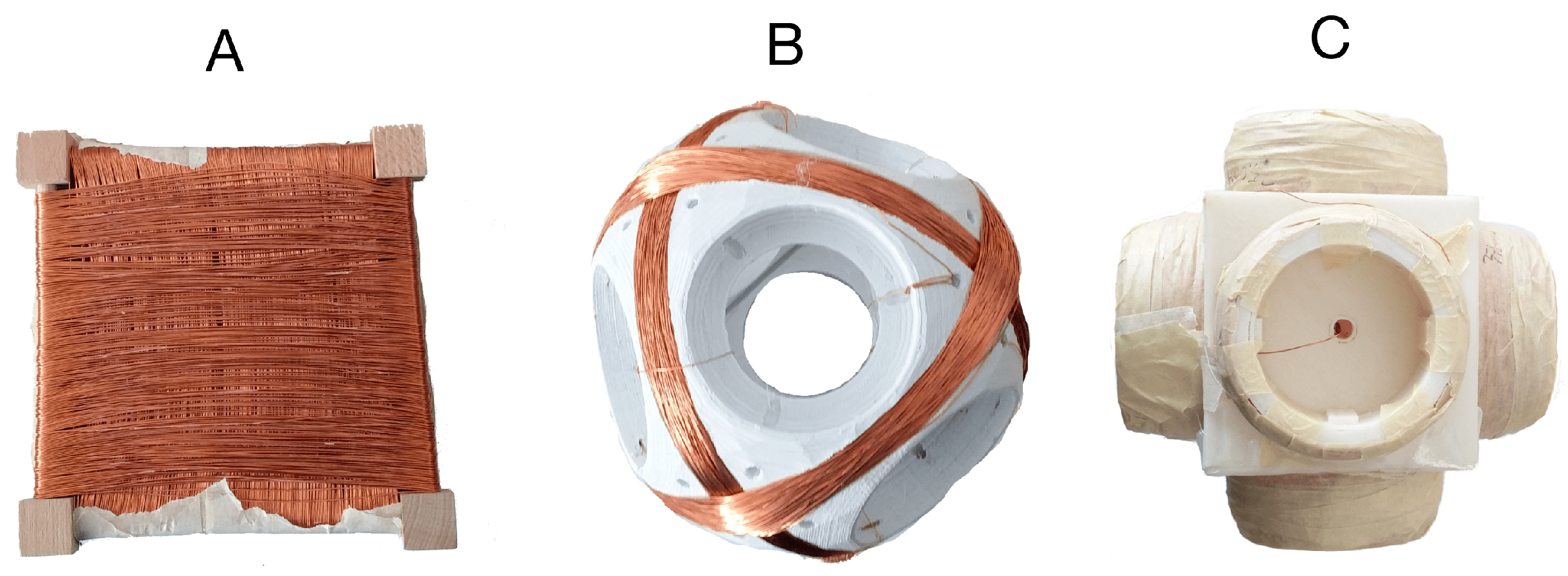
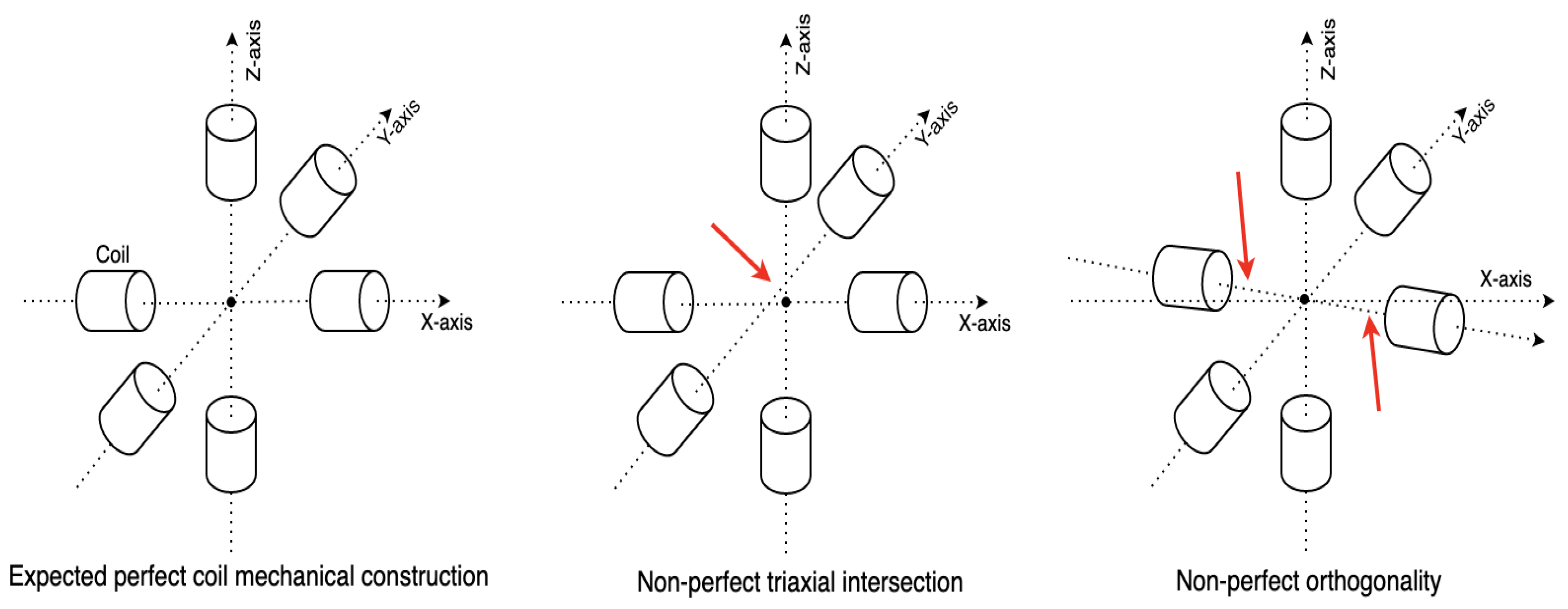
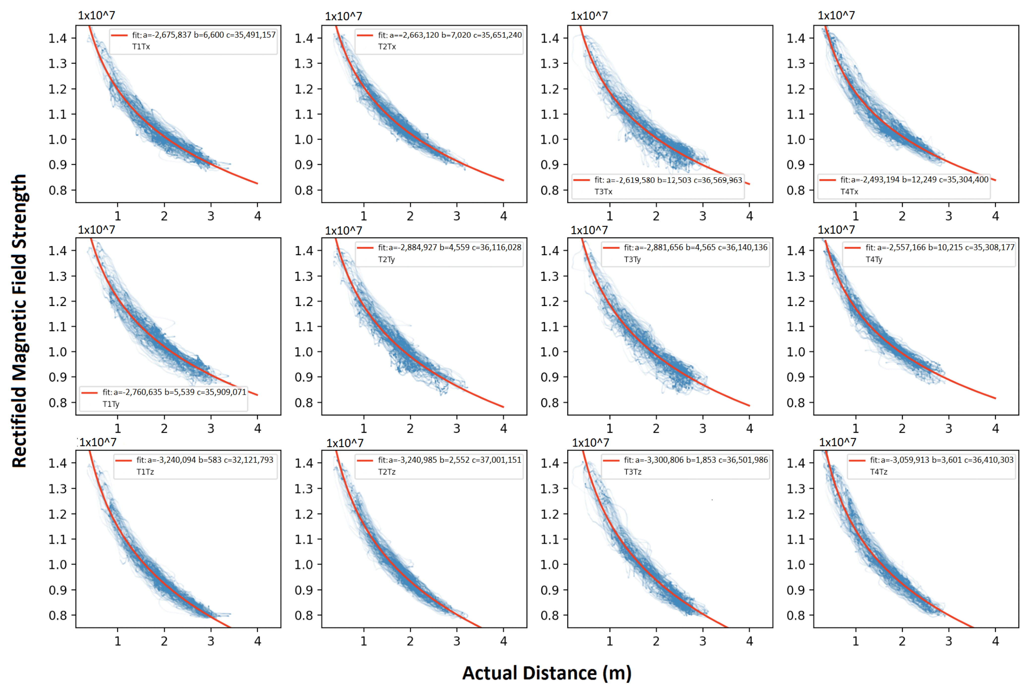
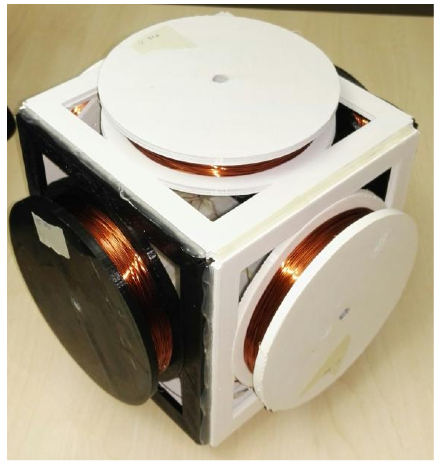
- We optimized the triaxial magnetic antenna (coils) regarding our previous work [23,24], significantly decreased the crosstalk of the magnetic field generated in each axis. We also redesigned the signal processing unit at the magnetic field strength sensing side and decreased the noise, thus improved the positioning accuracy.
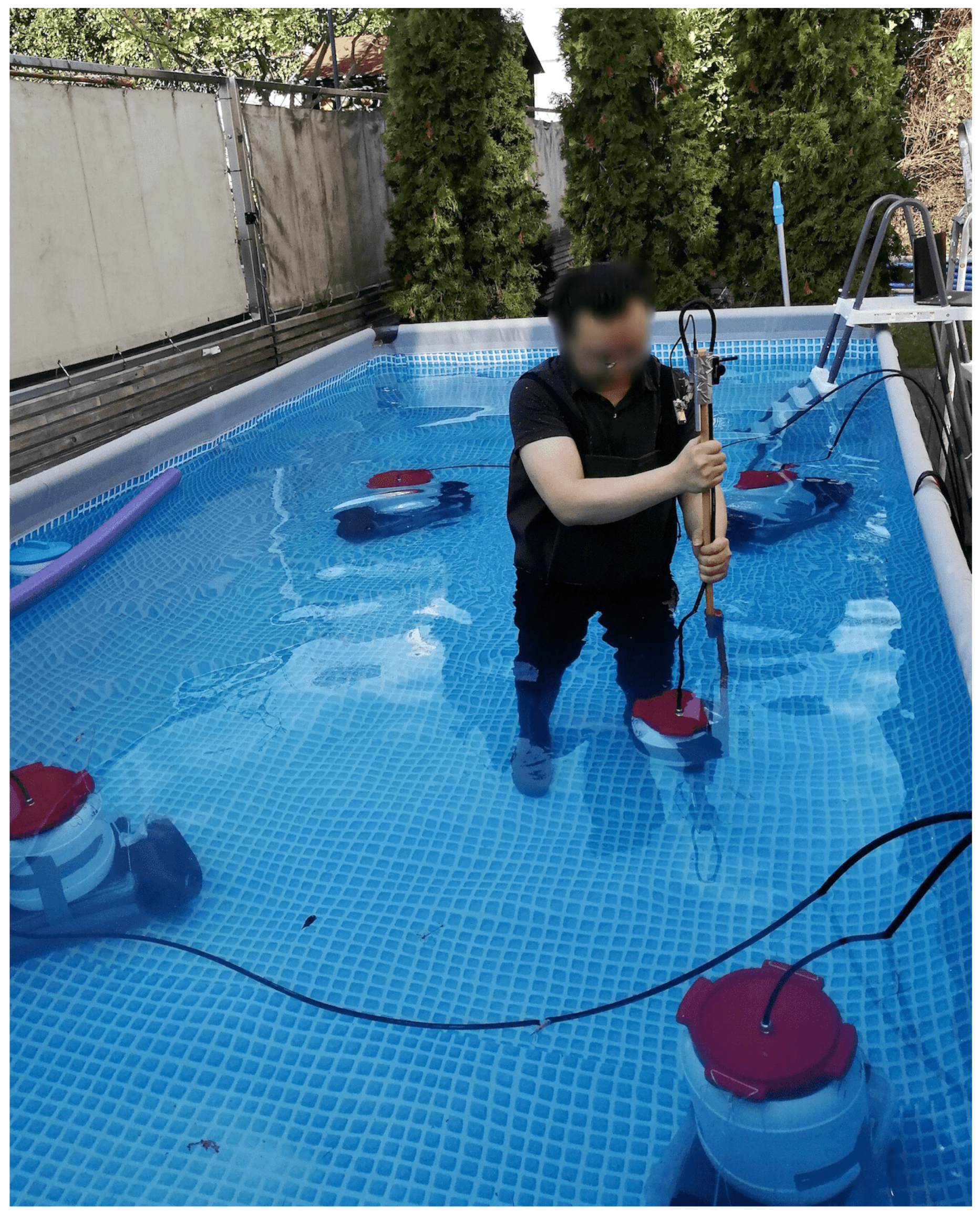
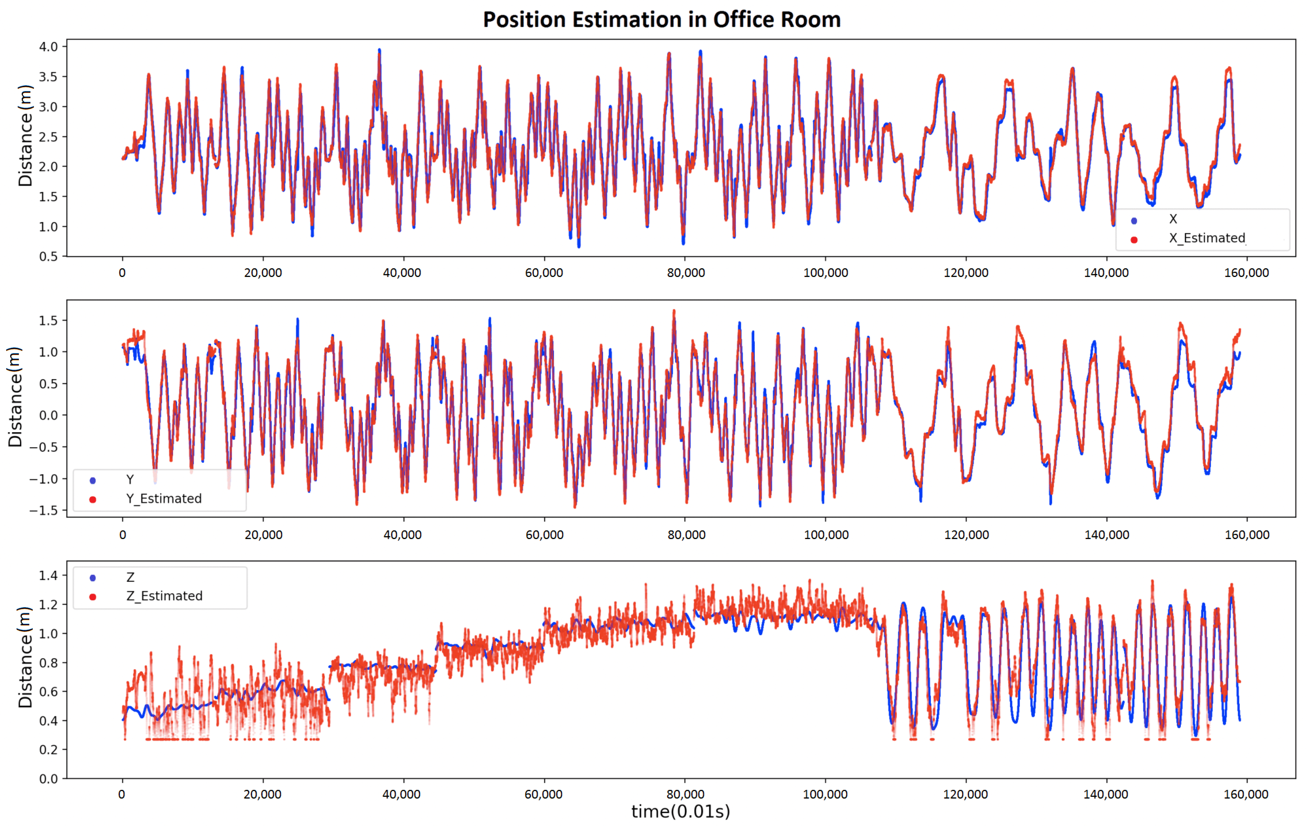
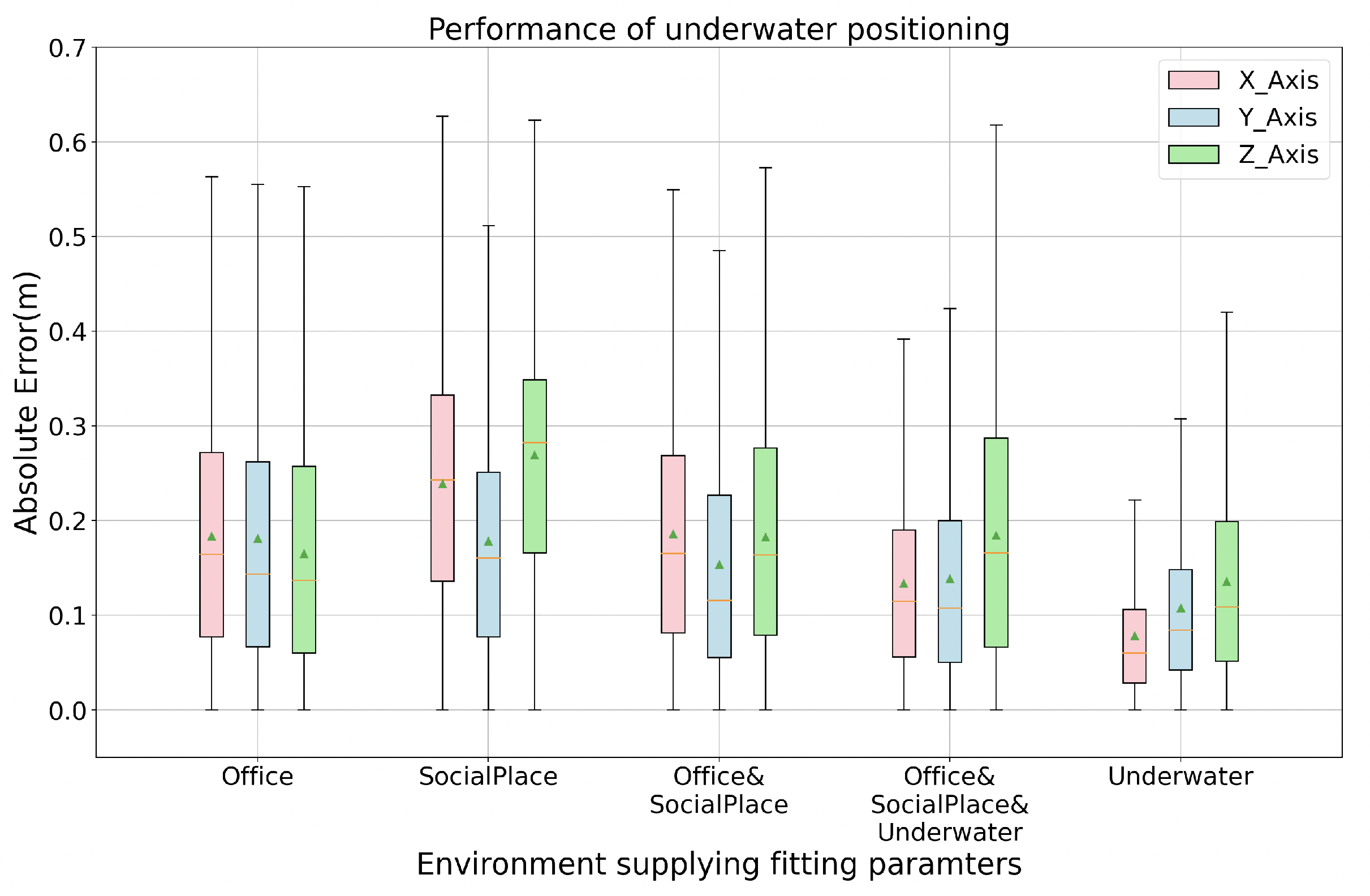
- We evaluated the magnetic-based positioning system in a swimming pool and compared the performance to full-equipped office room with chairs, tables, desktop computers, a social place with empty space, and a household. Evaluations show that the system can provide the positioning accuracy of 15.3 cm indoors and 13.3 cm underwater in 2D and 18.0 cm indoors and 19.0 cm underwater in 3D.
- The system is low cost, low power consumption, scalable for extensive coverage area, and could plug-and-play without pre-calibration.
2. Approach
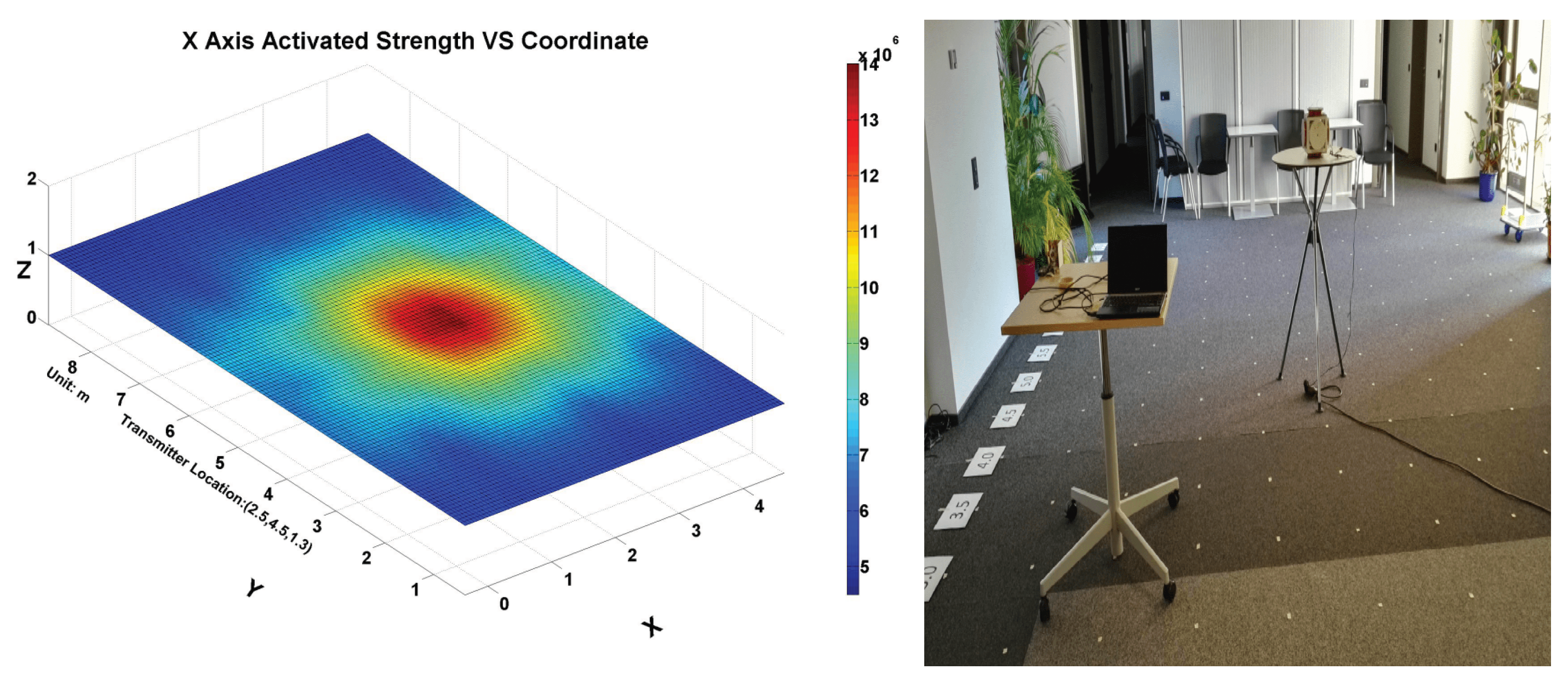
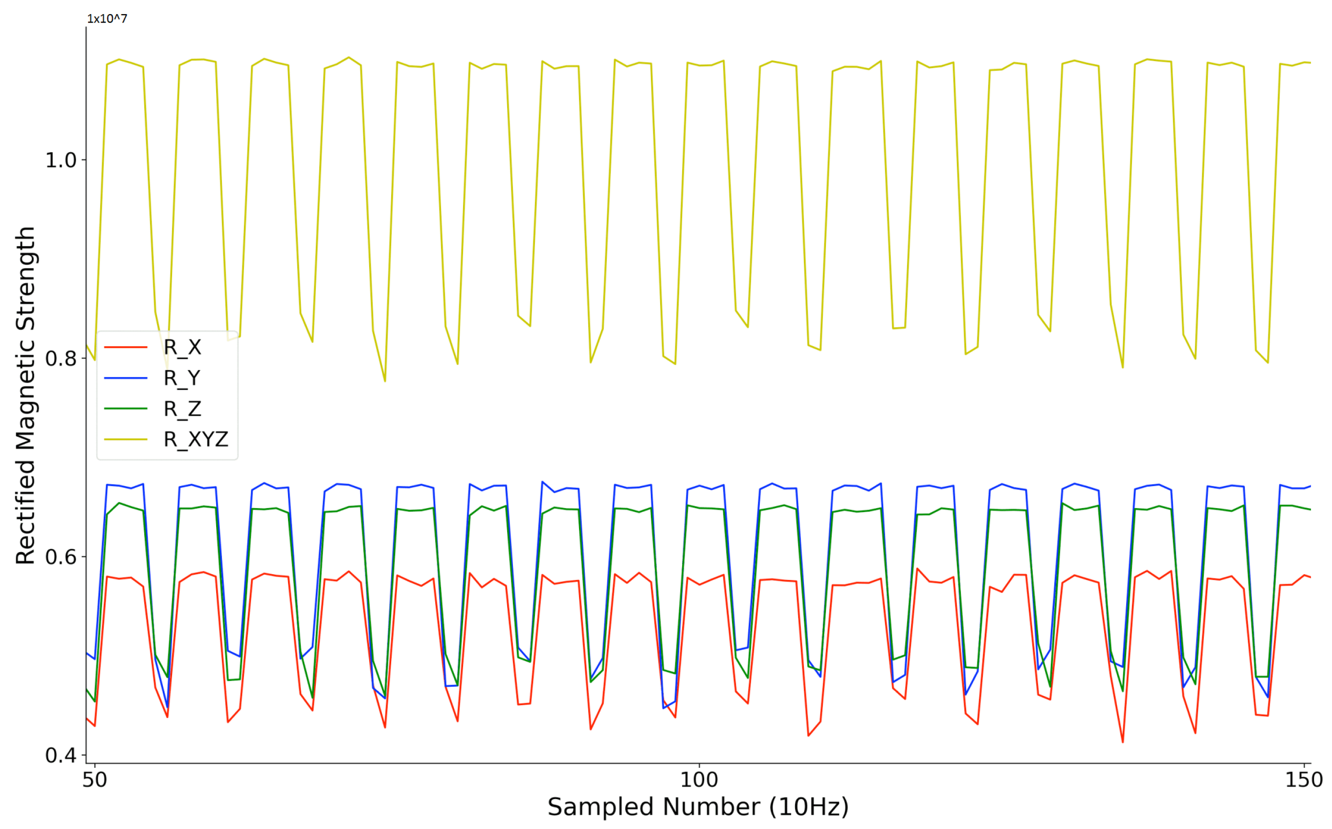
2.1. Physical Principle
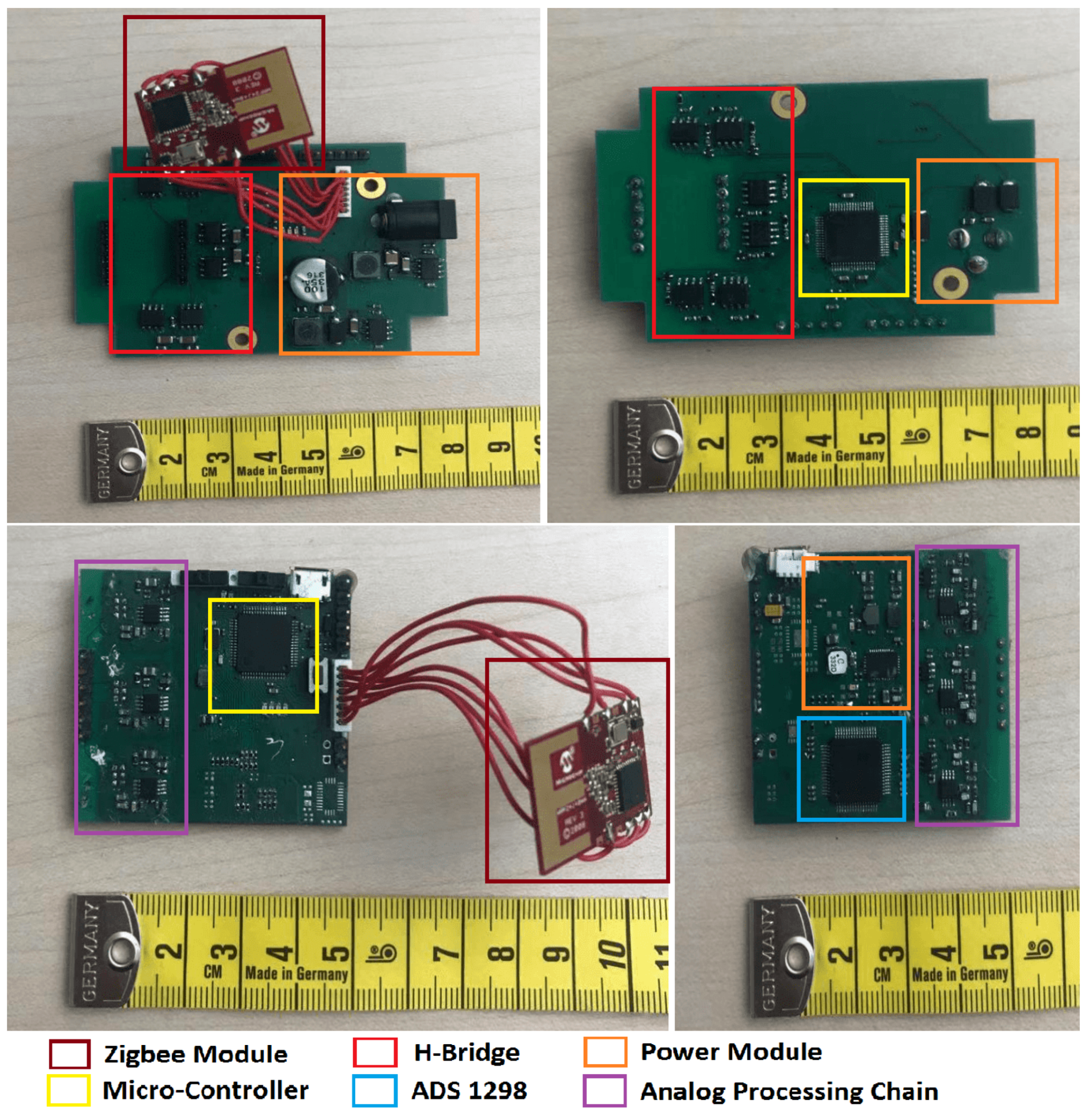
2.2. Transmitter and Receiver Coils
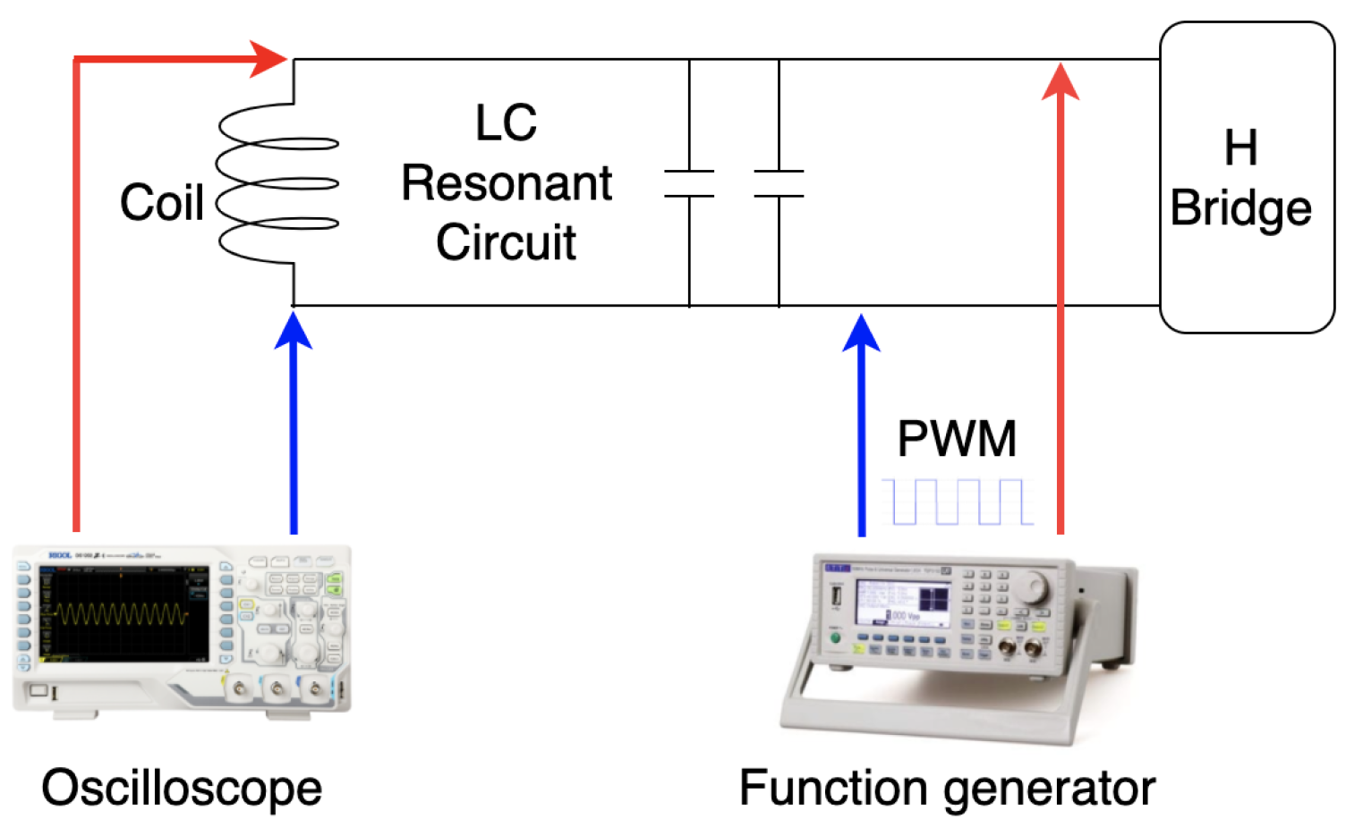
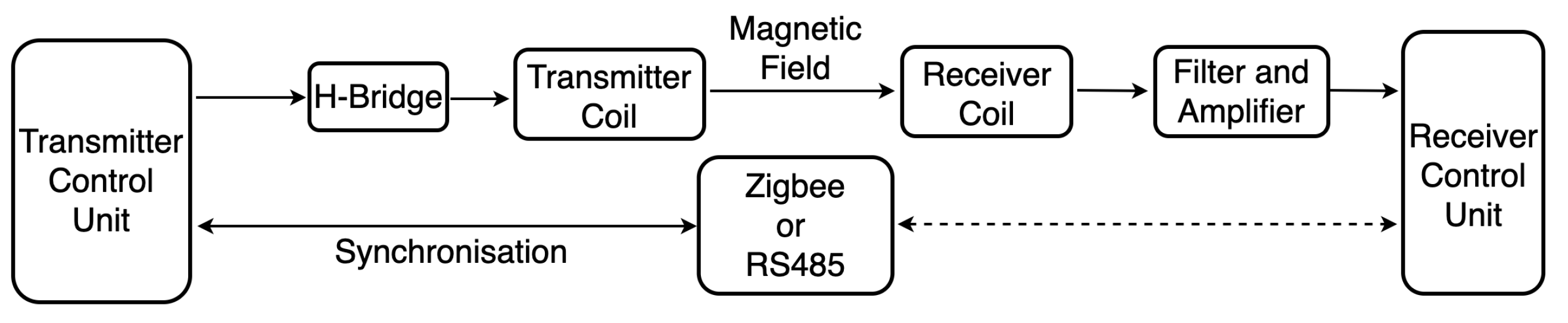
2.3. System Architecture
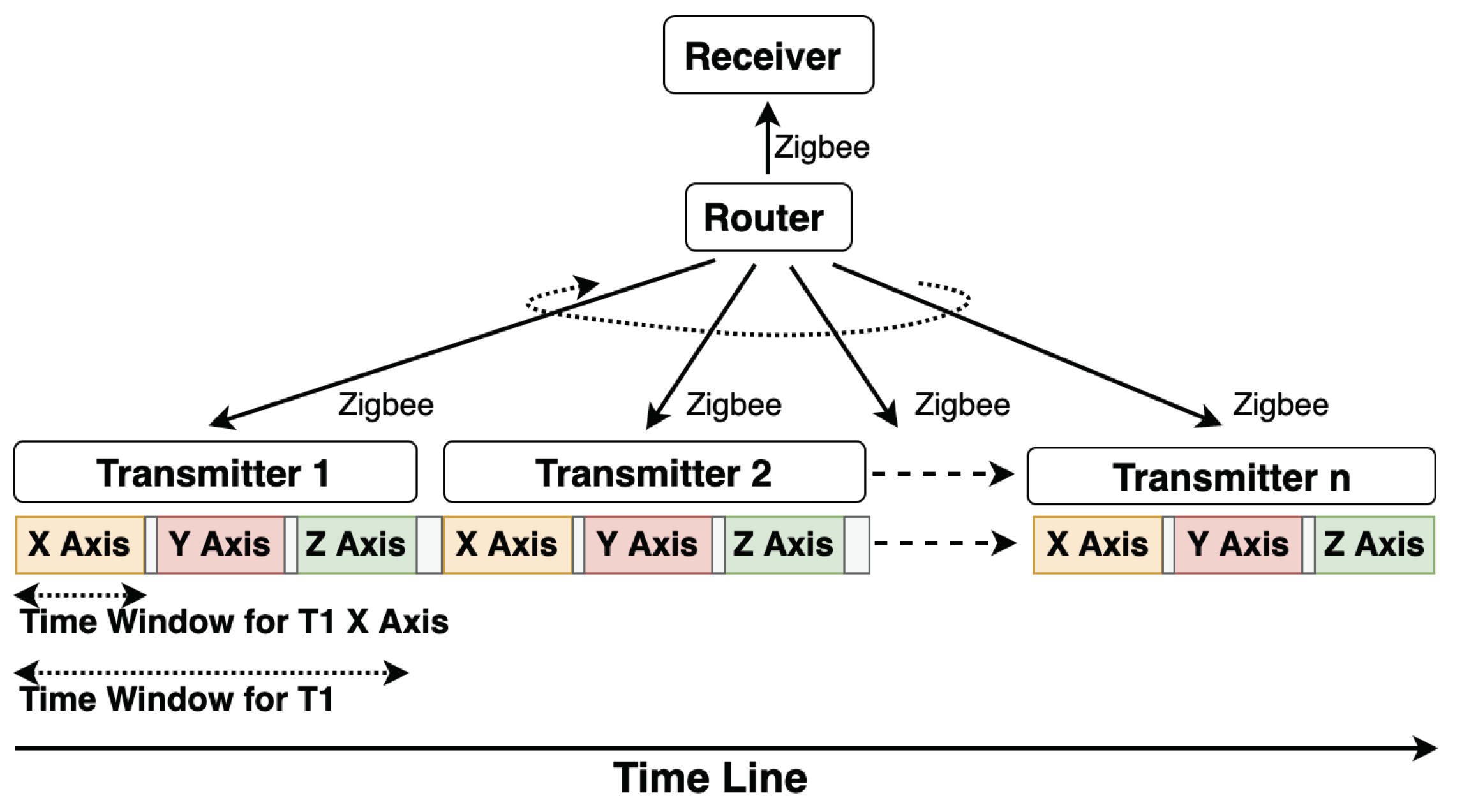
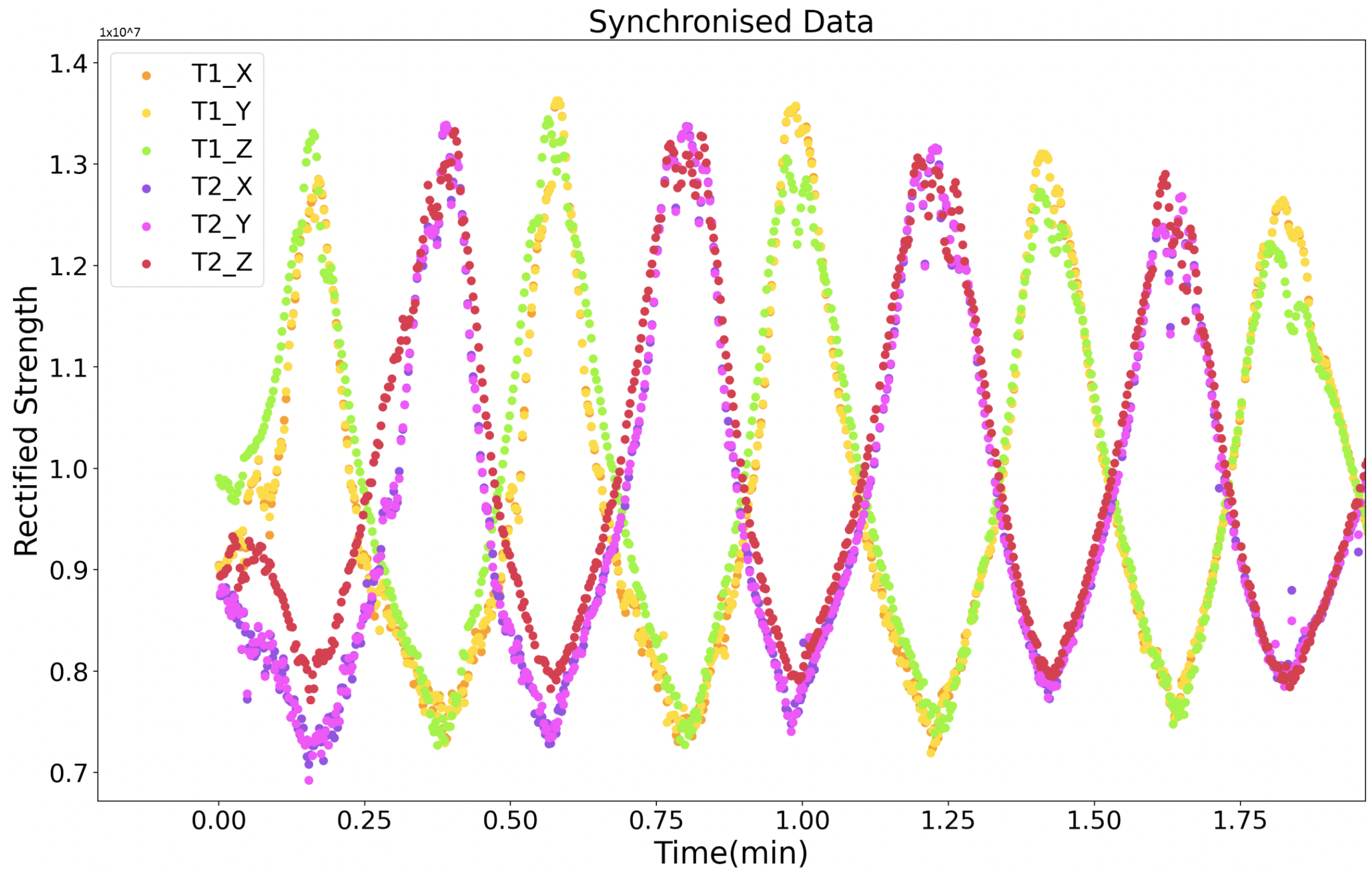
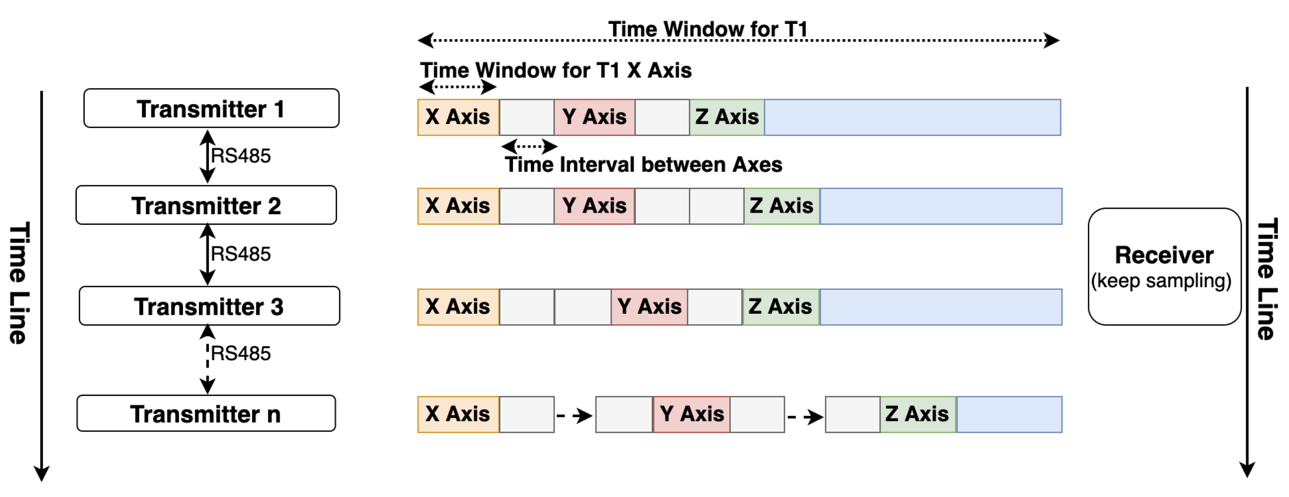
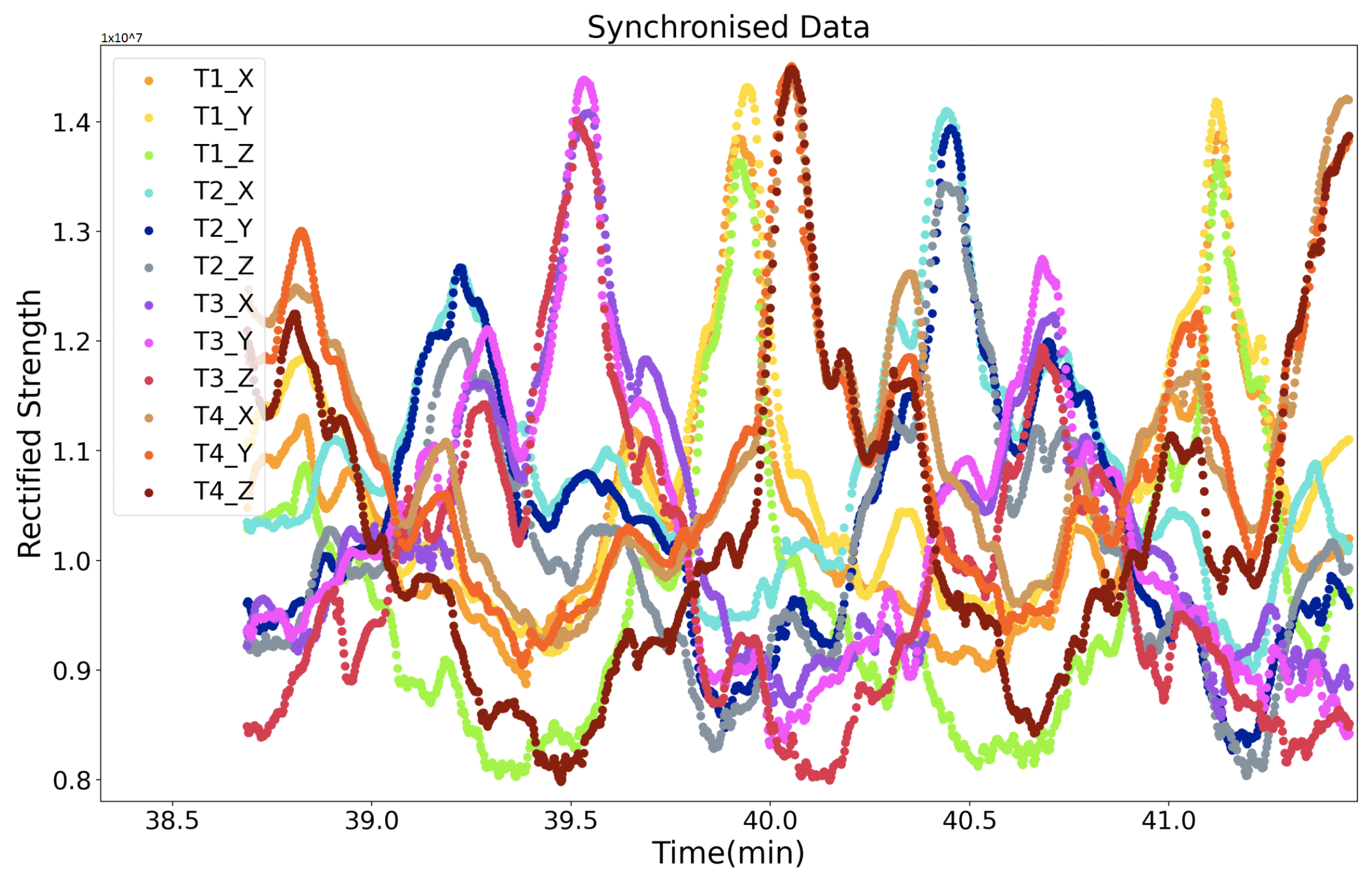
2.4. Transmitter Synchronization and Identification
2.4.1. Zigbee for Wireless Approach
2.4.2. RS485 for Wired Approach
2.4.3. Scalability of the System
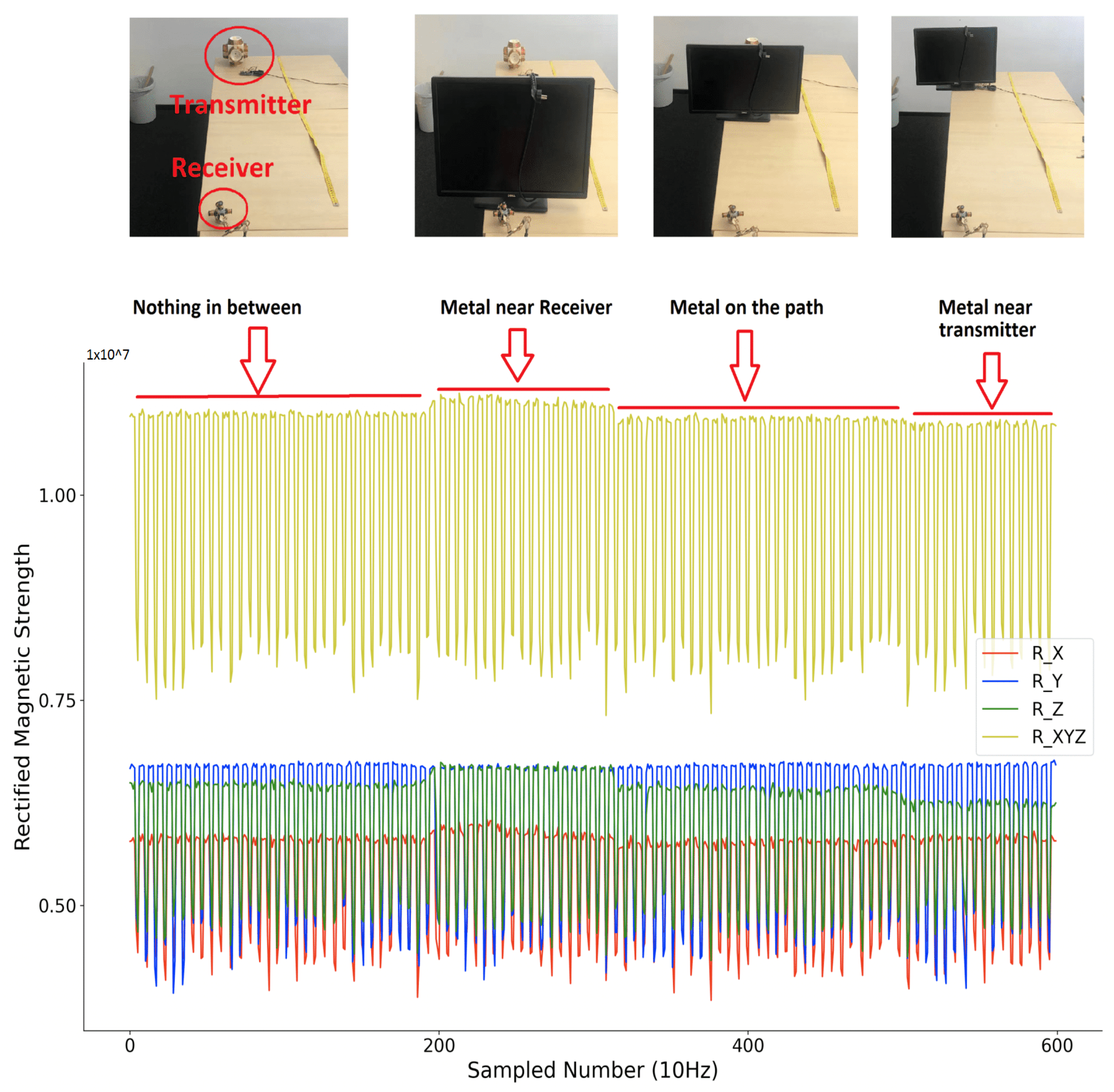
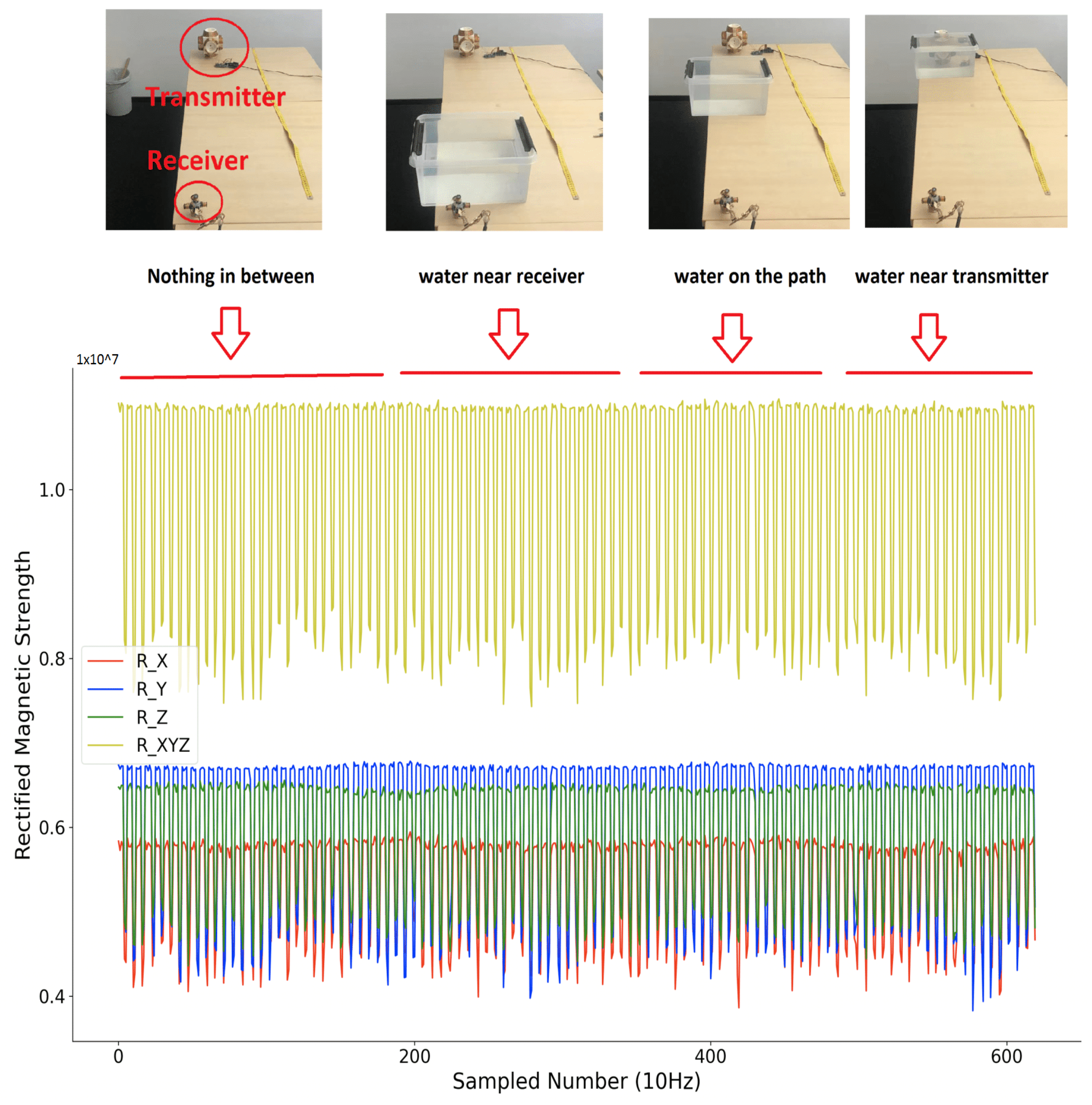
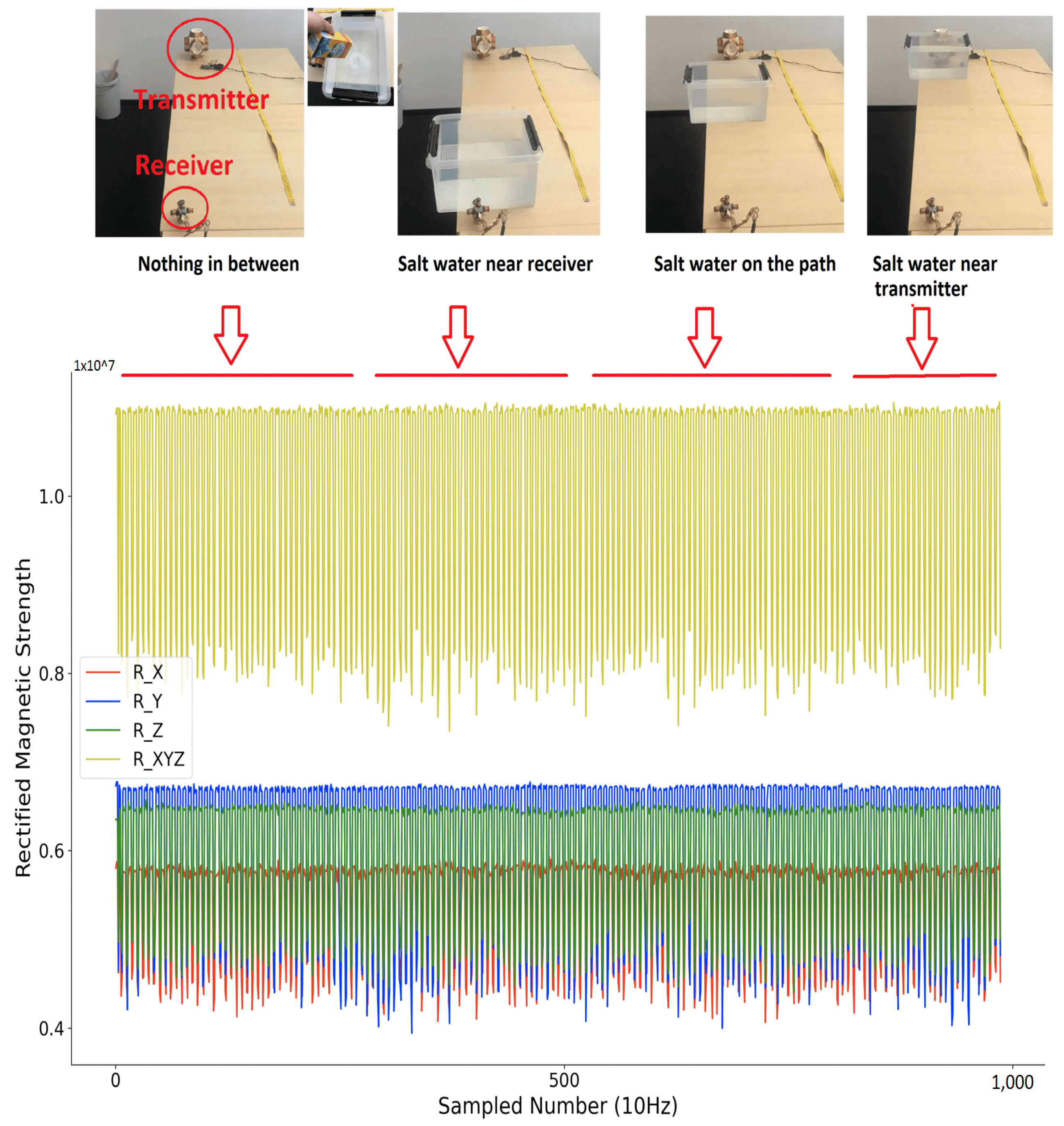
2.5. Preliminary Disturbance Test
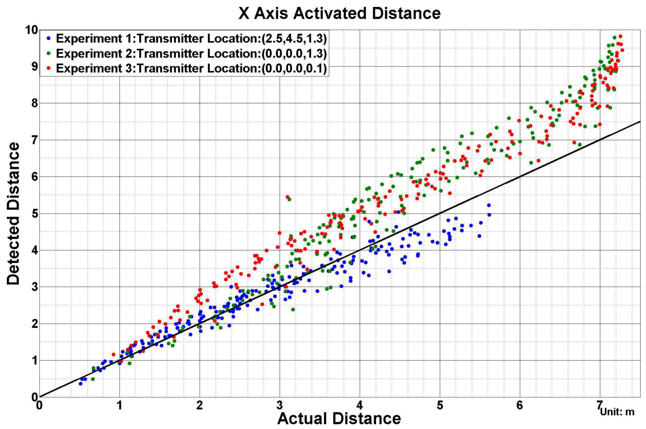
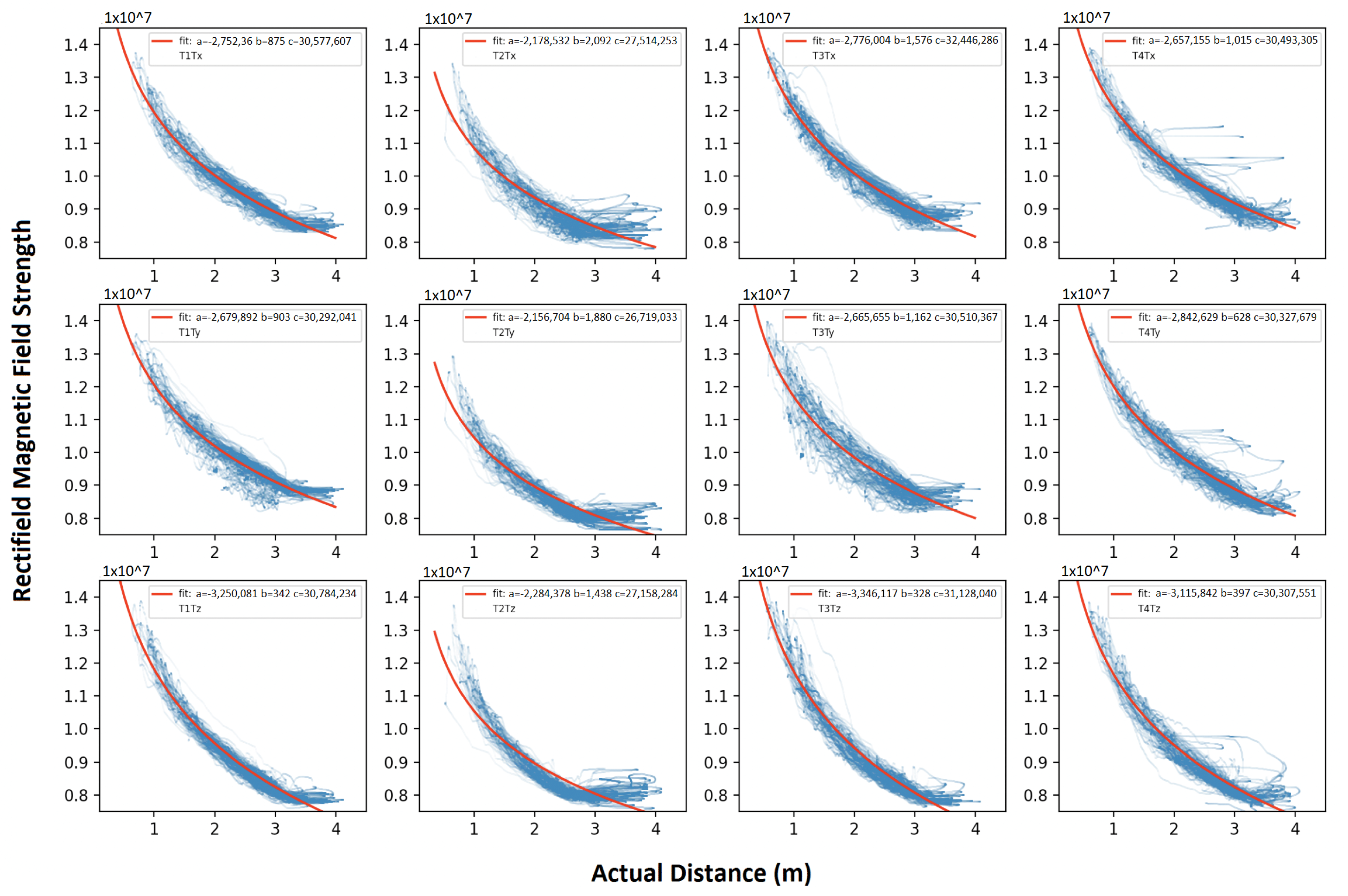
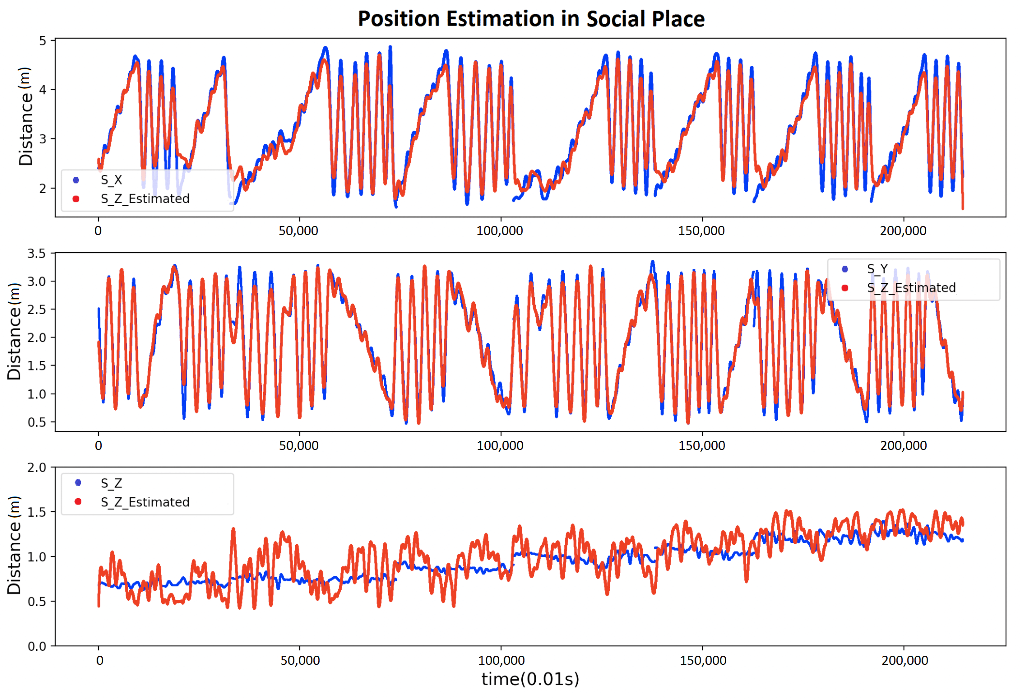
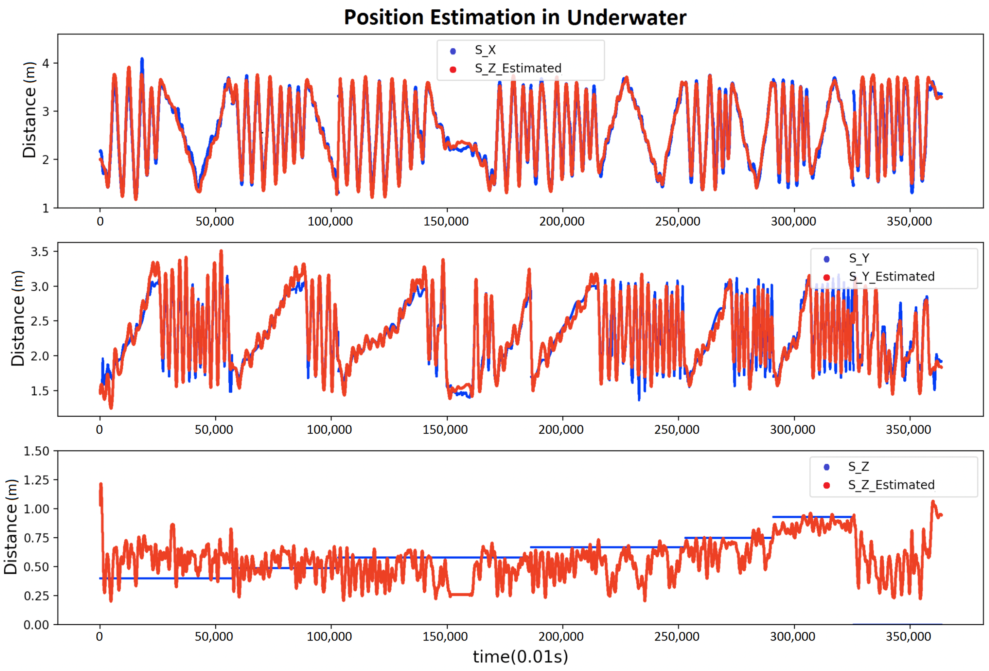
3. Evaluation
4. Conclusions and Future Work
Author Contributions
Funding
Institutional Review Board Statement
Informed Consent Statement
Data Availability Statement
Conflicts of Interest
Abbreviations
| ToF | Time of Flight |
| RSS | Received Signal Strength |
| LiDAR | Light and Radar |
| UWB | Ultra-wideband |
| RF | Radio Frequency |
| ID | Identification |
| MAE | Mean Absolute Error |
| IMU | Inertial Measurement Unit |
| PWM | Pulse-Width Modulation |
| AUV | Autonomous underwater vehicles |
| SLAM | Simultaneous localization and mapping |
Appendix A


References
- European Commission. The EU Blue Economy Report 2020; Technical Report; Publications Office of the European Union: Luxembourg, 2020. [Google Scholar]
- Verband für Schiffbau und Meerestechnik e.V.; VSM Jahresbericht 2018/2019; VSM Technical Report; VSM: Hamburg, Germany, 2019.
- Kampmann, P.; Christensen, L.; Fritsche, M.; Gaudig, C.; Hanff, H.; Hildebrandt, M.; Kirchner, F. How AI and Robotics can Support Marine Mining. In Proceedings of the Offshore Technology Conference (OTC-2018), Houston, TX, USA, 29 April–4 May 2018. [Google Scholar]
- Petillot, Y.R.; Antonelli, G.; Casalino, G.; Ferreira, F. Underwater Robots: From Remotely Operated Vehicles to Intervention-Autonomous Underwater Vehicles. IEEE Robot. Autom. Mag. 2019, 26, 94–101. [Google Scholar] [CrossRef]
- Napolitano, F.; Cretollier, F.; Pelletier, H. GAPS, Combined USBL + INS + GPS Tracking System for Fast Deployable High Accuracy Multiple Target Positioning; Europe Oceans: Brussels, Belgium, 2005; Volume 2, pp. 1415–1420. [Google Scholar]
- Zhao, S.; Wang, Z.; He, K.; Ding, N. Investigation on underwater positioning stochastic model based on acoustic ray incidence angle. Appl. Ocean. Res. 2018, 77, 69–77. [Google Scholar] [CrossRef]
- Reis, J.; Morgado, M.; Batista, P.; Oliveira, P.; Silvestre, C. Design and experimental validation of a USBL underwater acoustic positioning system. Sensors 2016, 16, 1491. [Google Scholar] [CrossRef] [PubMed] [Green Version]
- Kebkal, O.; Kebkal, K.; Bannasch, R. Long-baseline Hydro-acoustic positioning using D-MAC communication protocol. In Proceedings of the 2012 Oceans-Yeosu, Yeosu, Korea, 21–24 May 2012; pp. 1–7. [Google Scholar]
- Wu, Y.; Ta, X.; Xiao, R.; Wei, Y.; An, D.; Li, D. Survey of underwater robot positioning navigation. Appl. Ocean. Res. 2019, 90, 101845. [Google Scholar] [CrossRef]
- Islam, T.; Park, S.H. A Comprehensive Survey of the Recently Proposed Localization Protocols for Underwater Sensor Networks. IEEE Access 2020. [Google Scholar] [CrossRef]
- Morgado, M.; Oliveira, P.; Silvestre, C. Tightly coupled ultrashort baseline and inertial navigation system for underwater vehicles: An experimental validation. J. Field Robot. 2013, 30, 142–170. [Google Scholar] [CrossRef]
- Liu, S.; Ozay, M.; Okatani, T.; Xu, H.; Sun, K.; Lin, Y. Detection and pose estimation for short-range vision-based underwater docking. IEEE Access 2018, 7, 2720–2749. [Google Scholar] [CrossRef]
- Jia, Y.; Liu, T.; Gao, L.; Wang, D. Mobile robot localization and navigation system based on monocular vision. Trans. Tianjin Univ. 2012, 18, 335–342. [Google Scholar] [CrossRef]
- Akhoundi, F.; Minoofar, A.; Salehi, J.A. Underwater positioning system based on cellular underwater wireless optical CDMA networks. In Proceedings of the 2017 26th Wireless and Optical Communication Conference (WOCC), Newark, NJ, USA, 7–8 April 2017; pp. 1–3. [Google Scholar]
- Saeed, N.; Celik, A.; Al-Naffouri, T.Y.; Alouini, M.S. Underwater optical wireless communications, networking, and localization: A survey. Ad Hoc Netw. 2019, 94, 101935. [Google Scholar] [CrossRef] [Green Version]
- Aulinas, J.; Carreras, M.; Llado, X.; Salvi, J.; Garcia, R.; Prados, R.; Petillot, Y.R. Feature extraction for underwater visual SLAM. In Proceedings of the OCEANS 2011 IEEE-Spain, Santander, Spain, 6–9 June 2011; pp. 1–7. [Google Scholar]
- Chen, W.; Sun, R. Range-Only SLAM for Underwater Navigation System with Uncertain Beacons. In Proceedings of the 2018 10th International Conference on Modelling, Identification and Control (ICMIC), Guiyang, China, 2–4 July 2018; pp. 1–5. [Google Scholar]
- Yuan, X.; Martínez-Ortega, J.F.; Fernández, J.A.S.; Eckert, M. AEKF-SLAM: A new algorithm for robotic underwater navigation. Sensors 2017, 17, 1174. [Google Scholar] [CrossRef] [Green Version]
- Hildebrandt, M.; Gaudig, C.; Christensen, L.; Natarajan, S.; Hidalgo Carrió, J.; Merz Paranhos, P.; Kirchner, F. A Validation Process for Underwater Localization Algorithms. Int. J. Adv. Robot. Syst. 2014, 11, 138. [Google Scholar] [CrossRef]
- Kinsey, J.C.; Eustice, R.M.; Whitcomb, L.L. A survey of underwater vehicle navigation: Recent advances and new challenges. In Proceedings of the IFAC Conference of Manoeuvering and Control of Marine Craft, Lisbon, Portugal, 20–22 September 2006; Volume 88, pp. 1–12. [Google Scholar]
- Christensen, L.; Fritsche, M.; Albiez, J.; Kirchner, F. USBL pose estimation using multiple responders. In Proceedings of the OCEANS’10 IEEE SYDNEY, Sydney, Australia, 24–27 May 2010; pp. 1–9. [Google Scholar]
- Arnold, S.; Medagoda, L. Robust Model-Aided Inertial Localization for Autonomous Underwater Vehicles. In Proceedings of the 2018 IEEE International Conference on Robotics and Automation (ICRA), Brisbane, Australia, 21–25 May 2018; pp. 4889–4896. [Google Scholar]
- Pirkl, G.; Lukowicz, P. Resonant magnetic coupling indoor localization system. In Proceedings of the 2013 ACM conference on Pervasive and Ubiquitous Computing Adjunct Publication, Zurich, Switzerland, 8–12 September 2013; pp. 59–62. [Google Scholar]
- Pirkl, G.; Lukowicz, P. Robust, low cost indoor positioning using magnetic resonant coupling. In Proceedings of the 2012 ACM Conference on Ubiquitous Computing, Pittsburgh, PA, USA, 5–8 September 2012; pp. 431–440. [Google Scholar]
- Bian, S.; Zhou, B.; Bello, H.; Lukowicz, P. A wearable magnetic field based proximity sensing system for monitoring COVID-19 social distancing. In Proceedings of the 2020 International Symposium on Wearable Computers, Cancún, Mexico, 12–17 September 2020; pp. 22–26. [Google Scholar]
- Bian, S.; Zhou, B.; Lukowicz, P. Social distance monitor with a wearable magnetic field proximity sensor. Sensors 2020, 20, 5101. [Google Scholar] [CrossRef]
- Christensen, L. Robot Navigation in Distorted Magnetic Fields. Ph.D. Thesis, Faculty of Mathematics and Computer Science, University of Bremen, Bremen, Germany, 28 November 2019. [Google Scholar]
- Christensen, L.; Gaudig, C.; Kirchner, F. Distortion-robust distributed magnetometer for underwater pose estimation in confined UUVs. In Proceedings of the OCEANS 2015—MTS/IEEE Washington, Washington, DC, USA, 19–22 October 2015; pp. 1–8. [Google Scholar]
- Hildebrandt, M.; Christensen, L.; Kirchner, F. Combining cameras, magnetometers and machine-learning into a close-range localization system for docking and homing. In Proceedings of the OCEANS 2017—Anchorage, Anchorage, AK, USA, 18–21 September 2017; pp. 1–6. [Google Scholar]
- Guo, H.; Sun, Z.; Wang, P. Multiple frequency band channel modeling and analysis for magnetic induction communication in practical underwater environments. IEEE Trans. Veh. Technol. 2017, 66, 6619–6632. [Google Scholar] [CrossRef]
- Li, Y.; Wang, S.; Jin, C.; Zhang, Y.; Jiang, T. A survey of underwater magnetic induction communications: Fundamental issues, recent advances, and challenges. IEEE Commun. Surv. Tutor. 2019, 21, 2466–2487. [Google Scholar] [CrossRef]
- Akyildiz, I.F.; Wang, P.; Sun, Z. Realizing underwater communication through magnetic induction. IEEE Commun. Mag. 2015, 53, 42–48. [Google Scholar] [CrossRef]
- Xiang, X.; Yu, C.; Niu, Z.; Zhang, Q. Subsea cable tracking by autonomous underwater vehicle with magnetic sensing guidance. Sensors 2016, 16, 1335. [Google Scholar] [CrossRef] [Green Version]
- Callmer, J.; Skoglund, M.; Gustafsson, F. Silent localization of underwater sensors using magnetometers. Eurasip J. Adv. Signal Process. 2010, 2010, 1–8. [Google Scholar] [CrossRef] [Green Version]
- Groben, D.; Thongpull, K.; Kammara, A.C.; König, A. Neural Virtual Sensors for Adaptive Magnetic Localization of Autonomous Dataloggers. Adv. Artif. Neural Syst. 2015, 2014. [Google Scholar] [CrossRef] [Green Version]
- Marvelmind. Precise (±2 cm) Indoor Positioning and Navigation, 2020. Commercial Product. Available online: https://marvelmind.com/ (accessed on 22 March 2021).
- ESP32. A Feature-Rich MCU with Integrated Wi-Fi and Bluetooth Connectivity for a Wide-Range of Applications. Commercial Product. 2020. Available online: https://www.espressif.com/en/products/socs/esp32/ (accessed on 22 March 2021).
- Scipy. Minimization of Scalar Function of One or More Variables. Scipy Libaray. Available online: https://docs.scipy.org/doc/scipy/ (accessed on 22 March 2021).
- Savitzky-Golay. Savitzky-Golay Filter. Scipy Libaray. 2020. Available online: https://docs.scipy.org/doc/scipy/ (accessed on 22 March 2021).
- Wu, F.; Liang, Y.; Fu, Y.; Ji, X. A robust indoor positioning system based on encoded magnetic field and low-cost IMU. In Proceedings of the 2016 IEEE/ION Position, Location and Navigation Symposium (PLANS), Savannah, GA, USA, 11–14 April 2016; pp. 204–212. [Google Scholar]
- Pasku, V.; De Angelis, A.; Dionigi, M.; De Angelis, G.; Moschitta, A.; Carbone, P. A positioning system based on low-frequency magnetic fields. IEEE Trans. Ind. Electron. 2015, 63, 2457–2468. [Google Scholar] [CrossRef]
- Sheinker, A.; Ginzburg, B.; Salomonski, N.; Frumkis, L.; Kaplan, B.Z. Remote tracking of a magnetic receiver using low frequency beacons. Meas. Sci. Technol. 2014, 25, 105101. [Google Scholar] [CrossRef]
- Gulbahar, B.; Akan, O.B. A communication theoretical modeling and analysis of underwater magneto-inductive wireless channels. IEEE Trans. Wirel. Commun. 2012, 11, 3326–3334. [Google Scholar] [CrossRef]


| Transmitter Coil | Activated Axis | Voltage on X | Voltage on Y | Voltage on Z |
|---|---|---|---|---|
| Figure 1A | X | 232 | 155 (63%) | 137 (58%) |
| Y | 158 (68%) | 245 | 179 (67%) | |
| Z | 132 (57%) | 167 (68%) | 236 | |
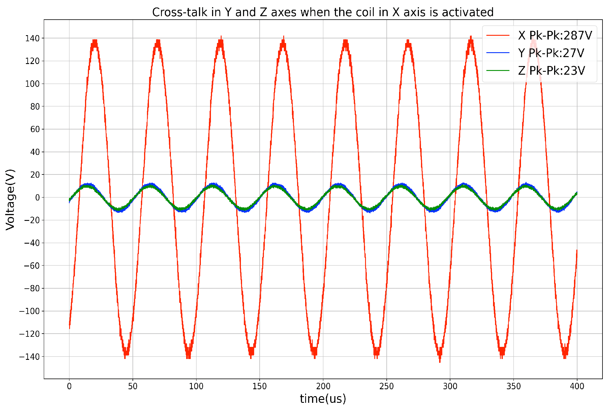
| Figure 1C | X | 287 | 21 (8%) | 30 (11%) |
| Y | 27 (9%) | 270 | 24 (9%) | |
| Z | 23 (8%) | 27 (10%) | 272 |
| Environment | X | Y | Z |
|---|---|---|---|
| Underwater | 0.078 (0.073) | 0.108 (0.091) | 0.136 (0.106) |
| Office | 0.099 (0.071) | 0.117 (0.085) | 0.095 (0.078) |
| Social Place | 0.164 (0.149) | 0.116 (0.093) | 0.153 (0.101) |
| Env-A | Env-B | X | Y | Z |
|---|---|---|---|---|
| Underwater | Office | 0.184 (0.128) | 0.181 (0.146) | 0.165 (0.123) |
| Underwater | SocialPlace | 0.239 (0.131) | 0.179 (0.125) | 0.269 (0.134) |
| Underwater | SocialPlace & Office | 0.186 (0.128) | 0.154 (0.129) | 0.183 (0.126) |
| Underwater | Underwater & SocialPlace & Office | 0.133 (0.101) | 0.139 (0.116) | 0.184 (0.135) |
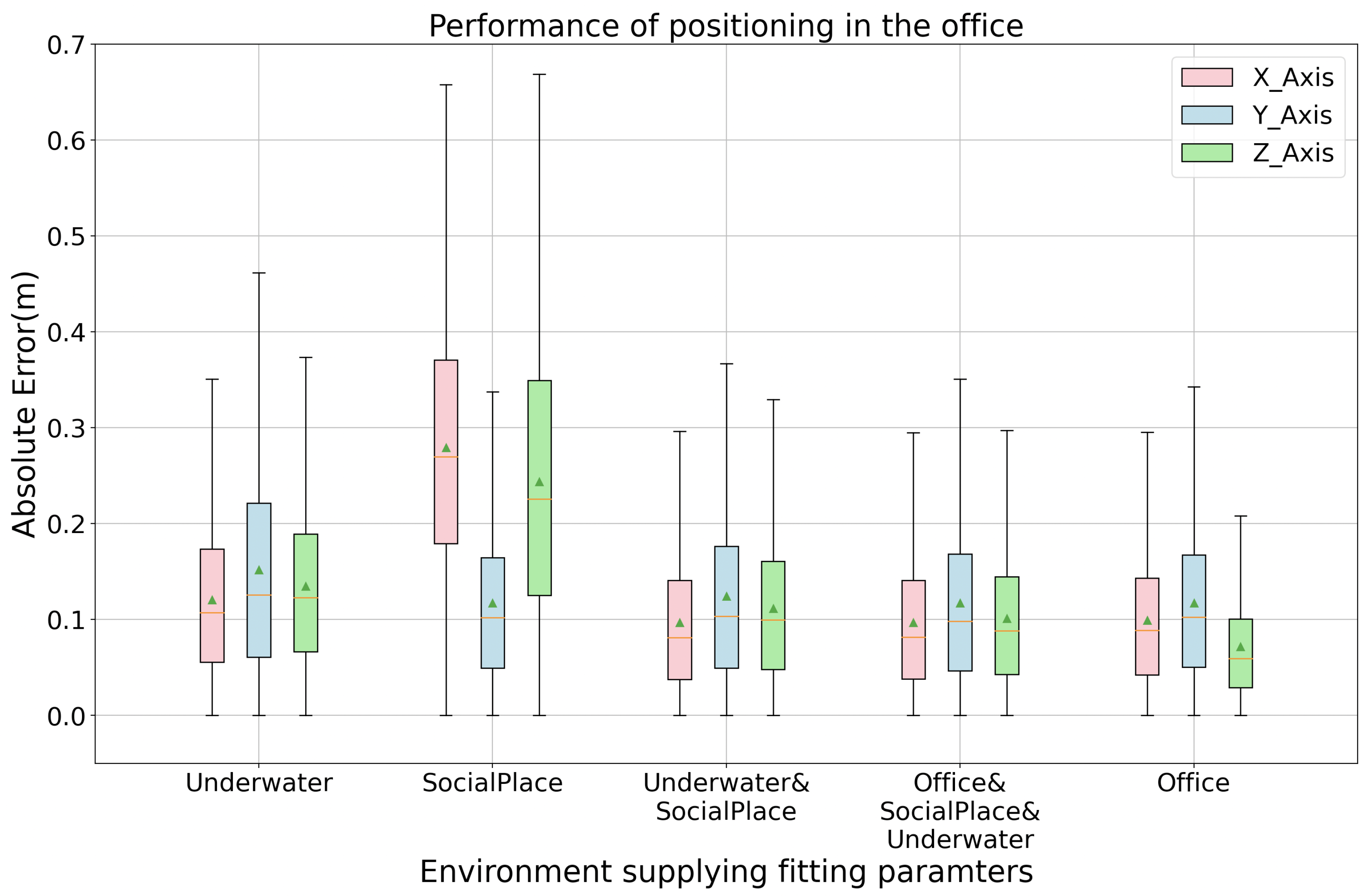
| Office | SocialPlace | 0.280 (0.142) | 0.117 (0.087) | 0.245 (0.149) |
| Office | Underwater | 0.121 (0.082) | 0.152 (0.115) | 0.135 (0.087) |
| Office | SocialPlace & Underwater | 0.097 (0.075) | 0.124 (0.096) | 0.111 (0.078) |
| Office | SocialPlace & Underwater & Office | 0.097 (0.074) | 0.117 (0.090) | 0.101 (0.073) |
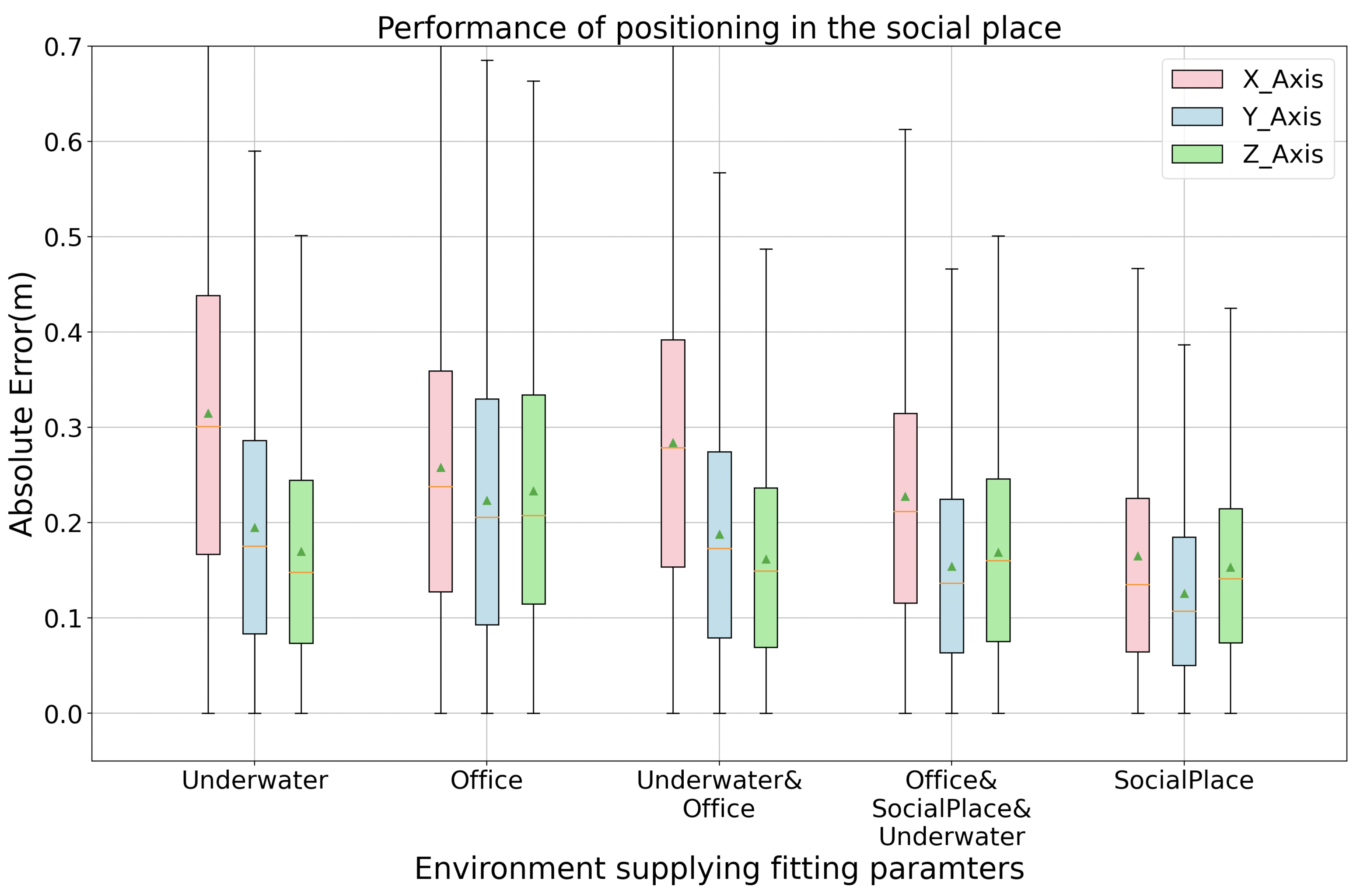
| SocialPlace | Office | 0.258 (0.166) | 0.220 (0.143) | 0.233 (0.152) |
| SocialPlace | Underwater | 0.315 (0.187) | 0.195 (0.134) | 0.170 (0.122) |
| SocialPlace | Underwater & Office | 0.285 (0.165) | 0.188 (0.129) | 0.162 (0.108) |
| SocialPlace | SocialPlace & Underwater & Office | 0.227 (0.148) | 0.154 (0.110) | 0.169 (0.110) |
Publisher’s Note: MDPI stays neutral with regard to jurisdictional claims in published maps and institutional affiliations. |
© 2021 by the authors. Licensee MDPI, Basel, Switzerland. This article is an open access article distributed under the terms and conditions of the Creative Commons Attribution (CC BY) license (http://creativecommons.org/licenses/by/4.0/).
Share and Cite
Bian, S.; Hevesi, P.; Christensen, L.; Lukowicz, P. Induced Magnetic Field-Based Indoor Positioning System for Underwater Environments. Sensors 2021, 21, 2218. https://doi.org/10.3390/s21062218
Bian S, Hevesi P, Christensen L, Lukowicz P. Induced Magnetic Field-Based Indoor Positioning System for Underwater Environments. Sensors. 2021; 21(6):2218. https://doi.org/10.3390/s21062218
Chicago/Turabian StyleBian, Sizhen, Peter Hevesi, Leif Christensen, and Paul Lukowicz. 2021. "Induced Magnetic Field-Based Indoor Positioning System for Underwater Environments" Sensors 21, no. 6: 2218. https://doi.org/10.3390/s21062218