
Modular MA-XRF Scanner Development in the Multi-Analytical Characterisation of a 17th Century Azulejo from Portugal †

 ,
,  ,
,  , ,
, ,  and
and
Abstract
:
1. Introduction
2. Materials and Methods
2.1. MA-XRF Scanning
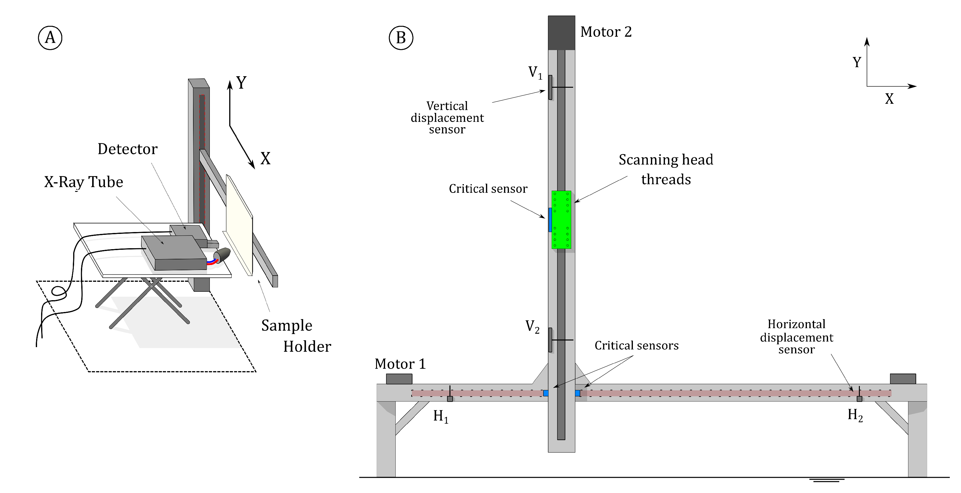
2.1.1. System Development
2.1.2. Data Acquisition
2.2. Monte Carlo Simulations
2.3. -Raman Analysis
3. Results and Discussion
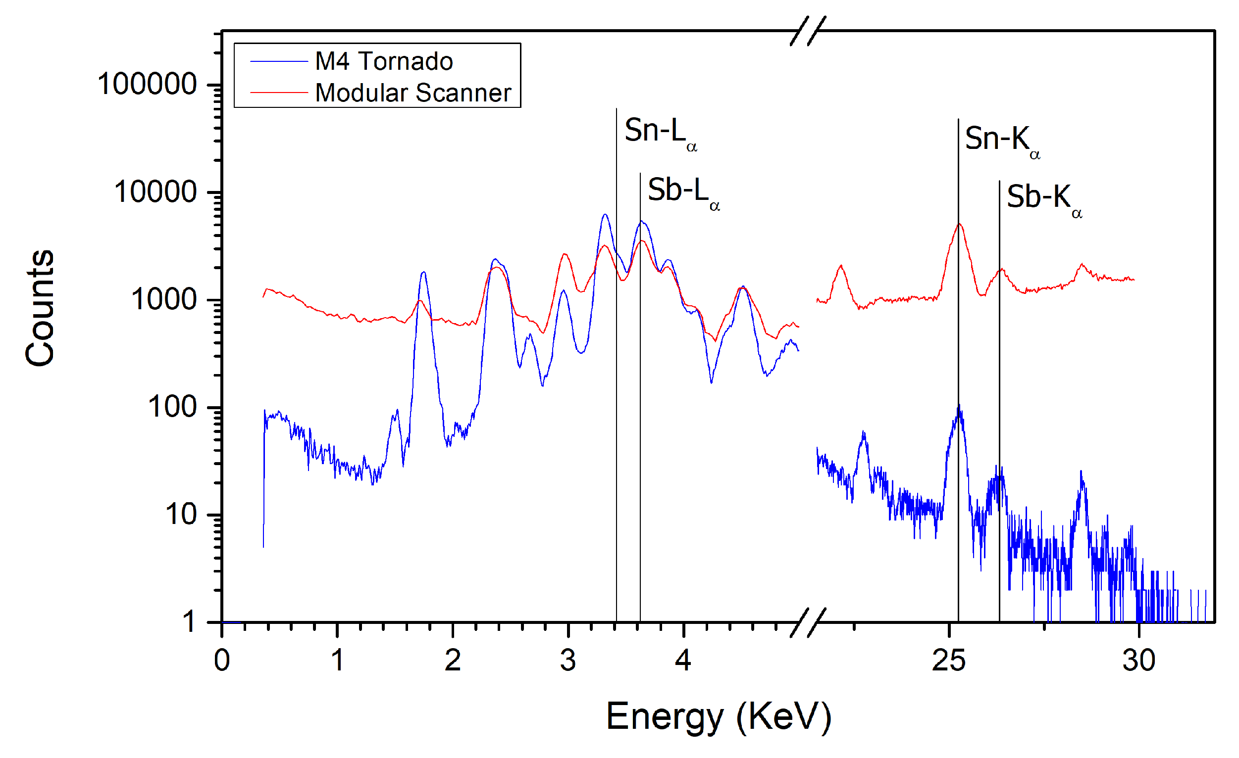
3.1. Scanner Performance
3.2. White Glaze
3.3. Blue Colour
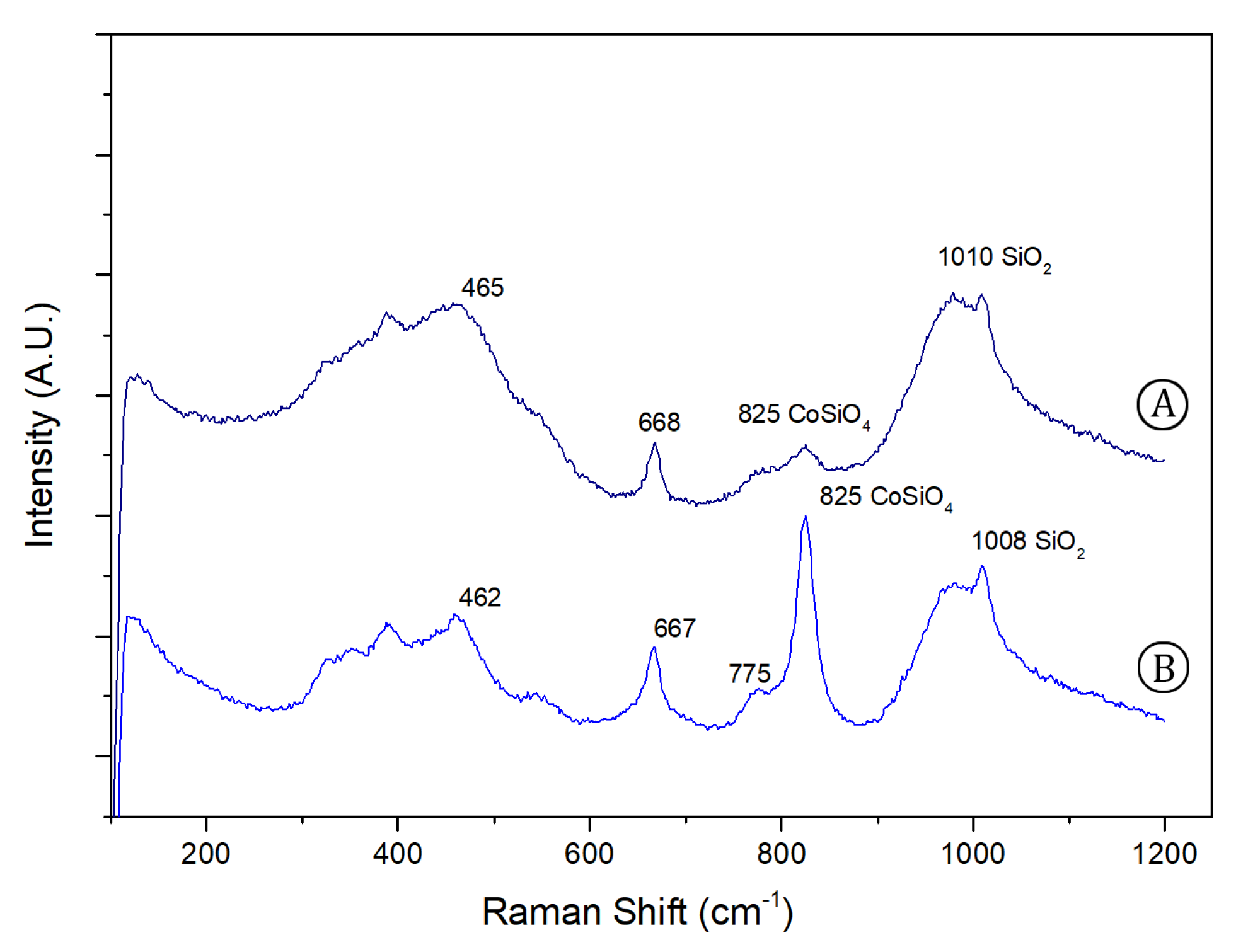
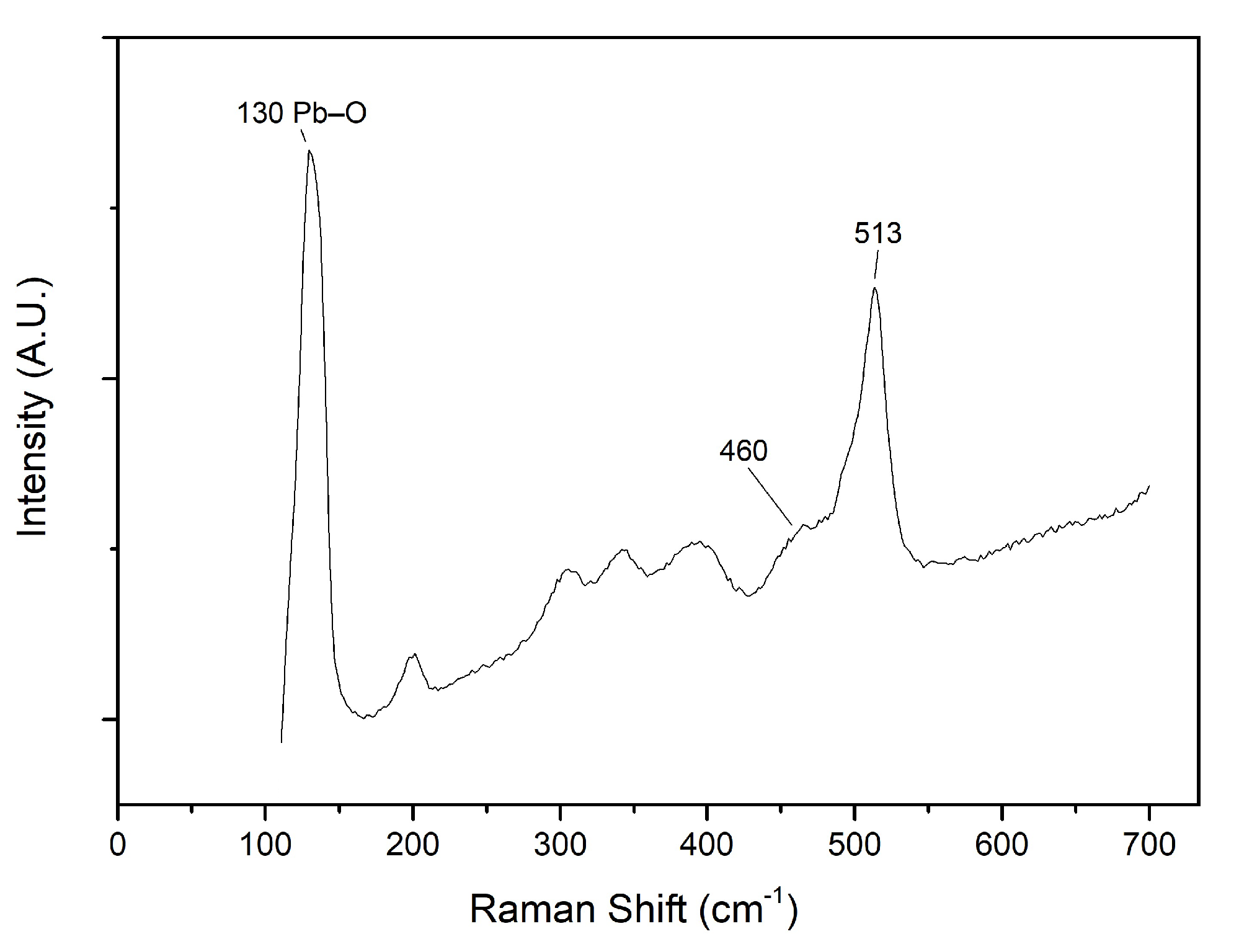
3.4. Yellow Colour
3.5. Orange Colour
4. Conclusions
Supplementary Materials
Author Contributions
Funding
Institutional Review Board Statement
Informed Consent Statement
Data Availability Statement
Acknowledgments
Conflicts of Interest
References
- Coentro, S.; Mimoso, J.M.; Lima, A.M.; Silva, A.S.; Pais, A.N.; Muralha, V.S. Multi-analytical identification of pigments and pigment mixtures used in 17th century Portuguese azulejos. J. Eur. Ceram. Soc. 2012, 32, 37–48. [Google Scholar] [CrossRef] [Green Version]
- Leal, A.S.; Alves, L.C.; Coentro, S.; Pereira, S.; Relvas, C.; Ferreira, T.; Mirão, J.; Fernandes, L.; Muralha, V.S. Caracterização química, física e mineralógica da colecção de azulejos hispano-mouriscos do Museu de Lisboa—Teatro Romano. Conservar Património 2018, 29, 25–39. [Google Scholar] [CrossRef] [Green Version]
- Barcellos Lins, S.A.; Manso, M.; Gigante, G.E.; Cesareo, R.; Tortora, L.; Branchini, P.; Ridolfi, S. Modular MA-XRF scanner potentialities and further advances. In Proceedings of the IMEKO International Conference on Metrology for Archaeology and Cultural Heritage, Trento, Italy, 22–24 October 2020; pp. 496–500. [Google Scholar]
- Mortari, C.; Nobre Pais, A.; Esteves, L.; Gago da Câmara, A.; Carvalho, M.L.; Manso, M. Raman and X-ray fluorescence glaze characterisation of Maria Keil’s decorative tile panels. J. Raman Spectrosc. 2021, 52, 59–70. [Google Scholar] [CrossRef]
- Mimoso, J.M.; Pais, A.; Ferreira, M.; Esteves, M.d.L.; Pereira, S.R.M.; Antunes, M.A.; Valona, R.; Cardoso, A.M.; Candeias, A. Instrumental Study of the 16th Century Azulejo Panel Decorating a Public Fountain in Alcacer do Sal-Portugal; LABORATÓRIO NACIONAL DE ENGENHARIA CIVIL, I.P. LNEC: Lisbon, Portugal, 2019; pp. 19–34. [Google Scholar]
- Barcellos Lins, S.A.; Gigante, G.E.; Cesareo, R.; Ridolfi, S.; Brunetti, A. Testing the Accuracy of the Calculation of Gold Leaf Thickness by MC Simulations and MA-XRF Scanning. Appl. Sci. 2020, 10, 3582. [Google Scholar] [CrossRef]
- Brunetti, A.; Golosio, B.; Schoonjans, T.; Oliva, P. Use of Monte Carlo simulations for cultural heritage X-ray fluorescence analysis. Spectrochim. Acta Part B At. Spectrosc. 2015, 108, 15–20. [Google Scholar] [CrossRef]
- Brunetti, A.; Fabian, J.; La Torre, C.W.; Schiavon, N. A combined XRF/Monte Carlo simulation study of multilayered Peruvian metal artifacts from the tomb of the Priestess of Chornancap. Appl. Phys. A 2016, 122, 571. [Google Scholar] [CrossRef]
- Ravaud, E.; Pichon, L.; Laval, E.; Gonzalez, V.; Eveno, M.; Calligaro, T. Development of a versatile XRF scanner for the elemental imaging of paintworks. Appl. Phys. A Mater. Sci. Process. 2016, 122, 1–7. [Google Scholar] [CrossRef]
- Dik, J.; Janssens, K.; Van Der Snickt, G.; Van Der Loeff, L.; Rickers, K.; Cotte, M. Visualization of a lost painting by Vincent van Gogh using synchrotron radiation based X-ray fluorescence elemental mapping. Anal. Chem. 2008, 80, 6436–6442. [Google Scholar] [CrossRef]
- Nervo, M.; Romano, F.P.; Caliri, C.; Piccirillo, A.; Triolo, P.; Demonte, D.; Gatti, A.; Vergallo, E.; Cardinali, M.; Ferrero, M. “Costruzione del viadotto”: MA-XRF in the pictorial executive technique of Agostino Bosia. X-ray Spectrom. 2020. [Google Scholar] [CrossRef]
- Turner, N.K.; Patterson, C.S.; MacLennan, D.K.; Trentelman, K. Visualizing underdrawings in medieval manuscript illuminations with macro-X-ray fluorescence scanning. X-Ray Spectrom. 2019, 48, 251–261. [Google Scholar] [CrossRef]
- Saverwyns, S.; Currie, C.; Lamas-Delgado, E. Macro X-ray fluorescence scanning (MA-XRF) as tool in the authentication of paintings. Microchem. J. 2018, 137, 139–147. [Google Scholar] [CrossRef]
- Impallaria, A.; Petrucci, F.; Chiozzi, S.; Evangelisti, F.; Squerzanti, S. A scanner for in situ X-ray radiography of large paintings: The case of “Paolo and Francesca” by G. Previati. Eur. Phys. J. Plus 2021, 136, 126. [Google Scholar] [CrossRef]
- Alberti, R.; Frizzi, T.; Bombelli, L.; Gironda, M.; Aresi, N.; Rosi, F.; Miliani, C.; Tranquilli, G.; Talarico, F.; Cartechini, L. CRONO: A fast and reconfigurable macro X-ray fluorescence scanner for in-situ investigations of polychrome surfaces. X-Ray Spectrom. 2017, 46, 297–302. [Google Scholar] [CrossRef] [Green Version]
- Campos, P.H.; Appoloni, C.R.; Rizzutto, M.A.; Leite, A.R.; Assis, R.F.; Santos, H.C.; Silva, T.F.; Rodrigues, C.L.; Tabacniks, M.H.; Added, N. A low-cost portable system for elemental mapping by XRF aiming in situ analyses. Appl. Radiat. Isot. 2019, 152, 78–85. [Google Scholar] [CrossRef]
- Hocquet, F.P.; Calvo, H.; Xicotencatl, A.C.; Micha, E.; Strivay, D. Elemental 2D imaging of paintings with a mobile EDXRF system. Anal. Bioanal. Chem. 2011, 399, 3109–3116. [Google Scholar] [CrossRef]
- Polese, C.; Dabagov, S.; Esposito, A.; Liedl, A.; Hampai, D.; Bartùli, C.; Ferretti, M. Proposal for a prototype of portable micro-XRF spectrometer. Nucl. Instrum. Methods Phys. Res. Sect. Beam Interact. Mater. Atoms 2015, 355, 281–284. [Google Scholar] [CrossRef]
- Shugar, A.N. Handheld Macro-XRF Scanning: Development of Collimators for Sub-mm Resolution; The Institute of Analytical Philately: Akron, OH, USA, 2020; Chapter 3; pp. 13–19. [Google Scholar]
- Barcellos Lins, S.A.; Ridolfi, S.; Gigante, G.E.; Cesareo, R.; Albini, M.; Riccucci, C.; Carlo, G.; Fabbri, A.; Branchini, P.; Tortora, L. Differential X-Ray Attenuation in MA-XRF Analysis for a Non-invasive Determination of Gilding Thickness. Front. Chem. 2020, 8, 175. [Google Scholar] [CrossRef] [PubMed]
- Barcellos Lins, S.A.; Bremmers, B.; Gigante, G.E. XISMuS—X-ray fluorescence imaging software for multiple samples. SoftwareX 2020, 12, 100621. [Google Scholar] [CrossRef]
- Brunetti, A.; Sanchez Del Rio, M.; Golosio, B.; Simionovici, A.; Somogyi, A. A library for X-ray-matter interaction cross sections for X-ray fluorescence applications. Spectrochim. Acta Part B At. Spectrosc. 2004, 59, 1725–1731. [Google Scholar] [CrossRef]
- Guerra, M.F. The Study of the Characterisation and Provenance of Coins and Other Metalwork Using XRF, PIXE and Activation Analysis; Elsevier: Amsterdam, The Netherlands, 2000; pp. 378–416. [Google Scholar] [CrossRef]
- Schiavon, N.; de Palmas, A.; Bulla, C.; Piga, G.; Brunetti, A. An Energy-Dispersive X-Ray Fluorescence Spectrometry and Monte Carlo simulation study of Iron-Age Nuragic small bronzes (“Navicelle”) from Sardinia, Italy. Spectrochim. Acta Part B At. Spectrosc. 2016, 123, 42–46. [Google Scholar] [CrossRef]
- Wang, Z.; Bovik, A. A universal image quality index. IEEE Signal Process. Lett. 2002, 9, 81–84. [Google Scholar] [CrossRef]
- Nilsson, J.; Akenine-Möller, T. Understanding SSIM. arXiv 2020, arXiv:2006.13846. [Google Scholar]
- Alfeld, M.; Janssens, K.; Dik, J.; De Nolf, W.; Van Der Snickt, G. Optimization of mobile scanning macro-XRF systems for the in situ investigation of historical paintings. J. Anal. At. Spectrom. 2011, 26, 899–909. [Google Scholar] [CrossRef]
- de Waal, D. Micro-Raman and portable Raman spectroscopic investigation of blue pigments in selected Delft plates (17–20th Century). J. Raman Spectrosc. 2009, 40, 2162–2170. [Google Scholar] [CrossRef]
- Vieira Ferreira, L.; Casimiro, T.; Colomban, P. Portuguese tin-glazed earthenware from the 17th century. Part 1: Pigments and glazes characterization. Spectrochim. Acta Part A Mol. Biomol. Spectrosc. 2013, 104, 437–444. [Google Scholar] [CrossRef]
- RRUFF Database. Available online: https://rruff.info/quartz/display=default/R150074 (accessed on 20 November 2020).
- Pereira, M.; de Lacerda-Arôso, T.; Gomes, M.; Mata, A.; Alves, L.; Colomban, P. Ancient Portuguese Ceramic Wall Tiles (“Azulejos”): Characterization of the Glaze and Ceramic Pigments. J. Nano Res. 2009, 8, 79–88. [Google Scholar] [CrossRef]
- Sakellariou, K.; Miliani, C.; Morresi, A.; Ombelli, M. Spectroscopic investigation of yellow majolica glazes. J. Raman Spectrosc. 2004, 35, 61–67. [Google Scholar] [CrossRef]
- Rosi, F.; Manuali, V.; Miliani, C.; Brunetti, B.G.; Sgamellotti, A.; Grygar, T.; Hradil, D. Raman scattering features of lead pyroantimonate compounds. Part I: XRD and Raman characterization of Pb2Sb2O7 doped with tin and zinc. J. Raman Spectrosc. 2009, 40, 107–111. [Google Scholar] [CrossRef]
- Sandalinas, C.; Ruiz-Moreno, S.; López-Gil, A.; Miralles, J. Experimental confirmation by Raman spectroscopy of a Pb-Sn-Sb triple oxide yellow pigment in sixteenth-century Italian pottery. J. Raman Spectrosc. 2006, 37, 1146–1153. [Google Scholar] [CrossRef]
- Picolpasso, C. I Tre Libri Dell’ Arte Del Vasajo, Nei Quali Si Tratta Non Solo La Pratica, Ma Brevemente Tutti I Secreti Di Essa Cosa Che Persino Al Di’ D’oggi E’ Stata Senpre Tenuta Ascosta—Primary Source Edition; Nabu Press: Charleston, SC, USA, 2014; p. 126. [Google Scholar]


| Element | MSE | SSIM | MSE | SSIM | MSE | SSIM | MSE | SSIM |
| Fe | 539.30 | 0.71 | - | - | - | - | - | - |
| Co | 556.82 | 0.68 | - | - | - | - | - | - |
| Ni | 678.35 | 0.44 | - | - | - | - | - | - |
| Zn | 781.04 | 0.40 | - | - | - | - | - | - |
| As | - | - | 1116.47 | 0.27 | - | - | - | - |
| Sn | 1673.41 | 0.11 | - | - | 1957.48 | 0.11 | - | - |
| Sb | 2194.59 | 0.21 | - | - | 1167.72 | 0.50 | - | - |
| Pb | - | - | - | - | 146.66 | 0.14 | 2883.70 | 0.12 |
Publisher’s Note: MDPI stays neutral with regard to jurisdictional claims in published maps and institutional affiliations. |
© 2021 by the authors. Licensee MDPI, Basel, Switzerland. This article is an open access article distributed under the terms and conditions of the Creative Commons Attribution (CC BY) license (http://creativecommons.org/licenses/by/4.0/).
Share and Cite
Lins, S.A.B.; Manso, M.; Lins, P.A.B.; Brunetti, A.; Sodo, A.; Gigante, G.E.; Fabbri, A.; Branchini, P.; Tortora, L.; Ridolfi, S. Modular MA-XRF Scanner Development in the Multi-Analytical Characterisation of a 17th Century Azulejo from Portugal. Sensors 2021, 21, 1913. https://doi.org/10.3390/s21051913
Lins SAB, Manso M, Lins PAB, Brunetti A, Sodo A, Gigante GE, Fabbri A, Branchini P, Tortora L, Ridolfi S. Modular MA-XRF Scanner Development in the Multi-Analytical Characterisation of a 17th Century Azulejo from Portugal. Sensors. 2021; 21(5):1913. https://doi.org/10.3390/s21051913
Chicago/Turabian StyleLins, Sergio Augusto Barcellos, Marta Manso, Pedro Augusto Barcellos Lins, Antonio Brunetti, Armida Sodo, Giovanni Ettore Gigante, Andrea Fabbri, Paolo Branchini, Luca Tortora, and Stefano Ridolfi. 2021. "Modular MA-XRF Scanner Development in the Multi-Analytical Characterisation of a 17th Century Azulejo from Portugal" Sensors 21, no. 5: 1913. https://doi.org/10.3390/s21051913