Author Contributions
Conceptualization, A.K.; methodology, A.K.; software, A.K.; validation, A.K.; formal analysis, A.K.; investigation, A.K.; resources, A.K., M.V., and J.T.; data curation, A.K.; writing—original draft preparation, A.K., M.V., and J.T.; writing—review and editing, A.K., M.V., and J.T.; visualization, A.K.; supervision, M.V. and J.T.; project administration, M.V. and J.T.; funding acquisition, M.V. and J.T. All authors have read and agreed to the published version of the manuscript.
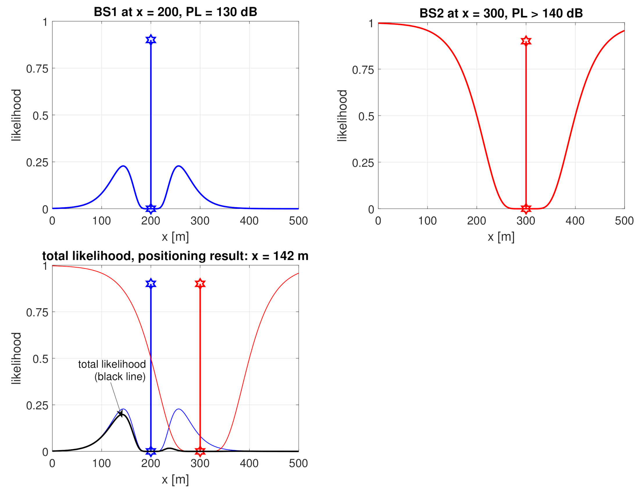
Figure 1.
Likelihood function illustration example in 1D: measured path loss (PL) of 130 dB to BS1, censored PL dB to BS2, and the combined likelihood function. Note that one measured and one censored PL are sufficient to get a unique positioning solution and the same is true in 2D and 3D.
Figure 1.
Likelihood function illustration example in 1D: measured path loss (PL) of 130 dB to BS1, censored PL dB to BS2, and the combined likelihood function. Note that one measured and one censored PL are sufficient to get a unique positioning solution and the same is true in 2D and 3D.
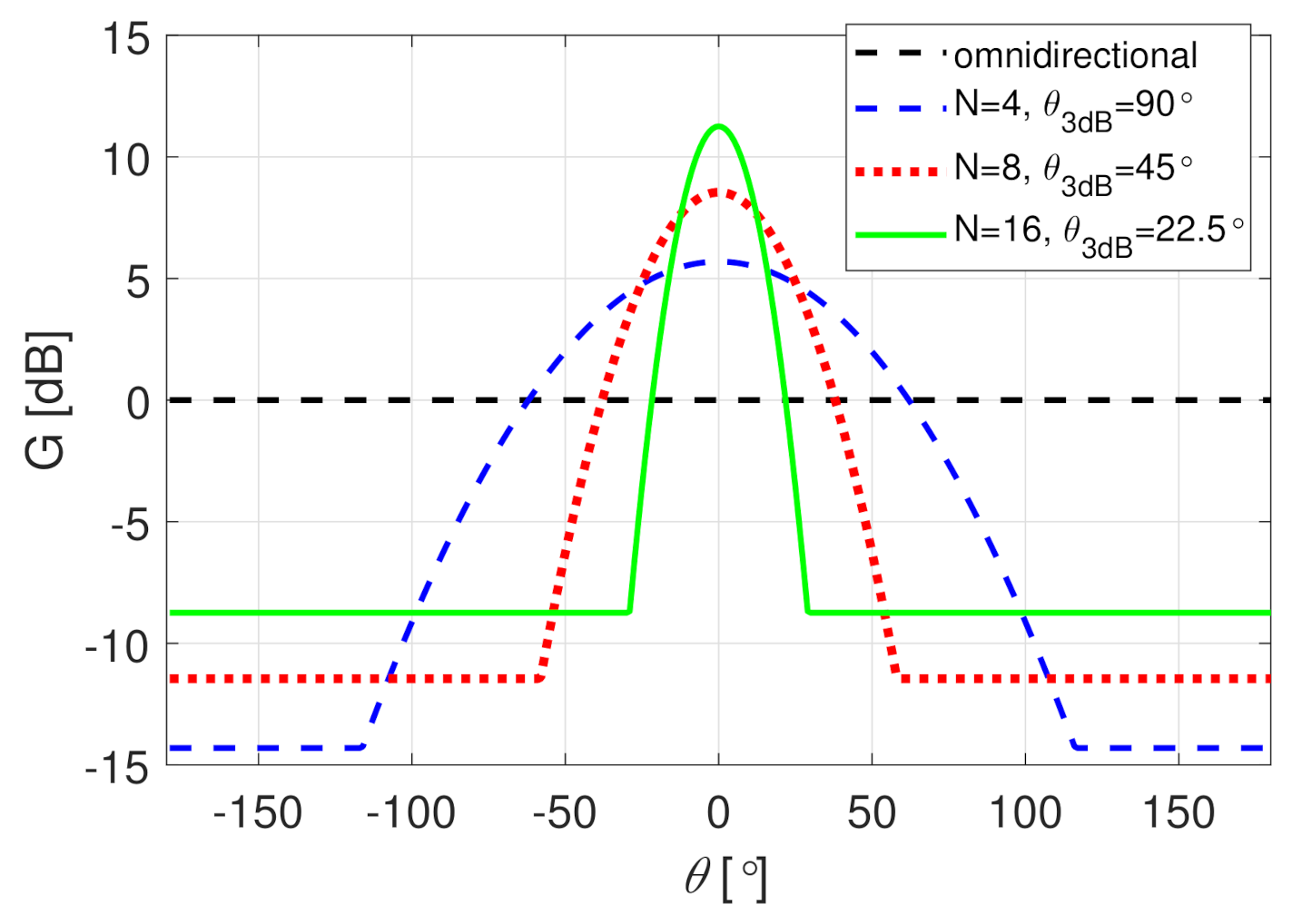
Figure 2.
Antenna gain as a function of the offset angle . The directive beam patterns have beam-width of .
Figure 2.
Antenna gain as a function of the offset angle . The directive beam patterns have beam-width of .
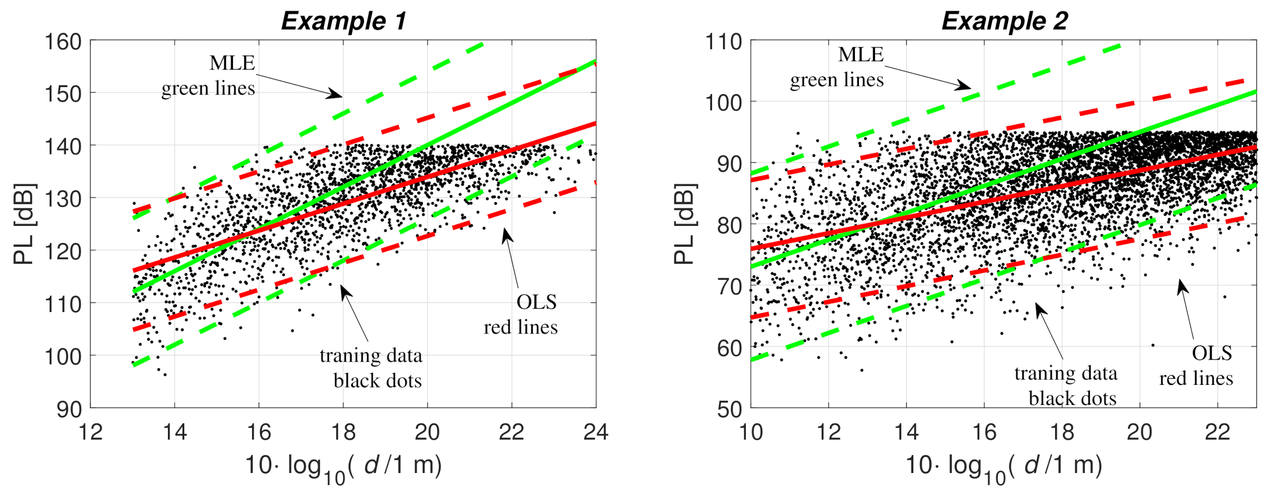
Figure 3.
Fitting the path loss model to the training data with OLS (green) and MLE (red)—Example 1 (, , ) and Example 2 (, ). Training data with under the noise threshold are shown with black dots, solid lines show , and the dash lines are .
Figure 3.
Fitting the path loss model to the training data with OLS (green) and MLE (red)—Example 1 (, , ) and Example 2 (, ). Training data with under the noise threshold are shown with black dots, solid lines show , and the dash lines are .
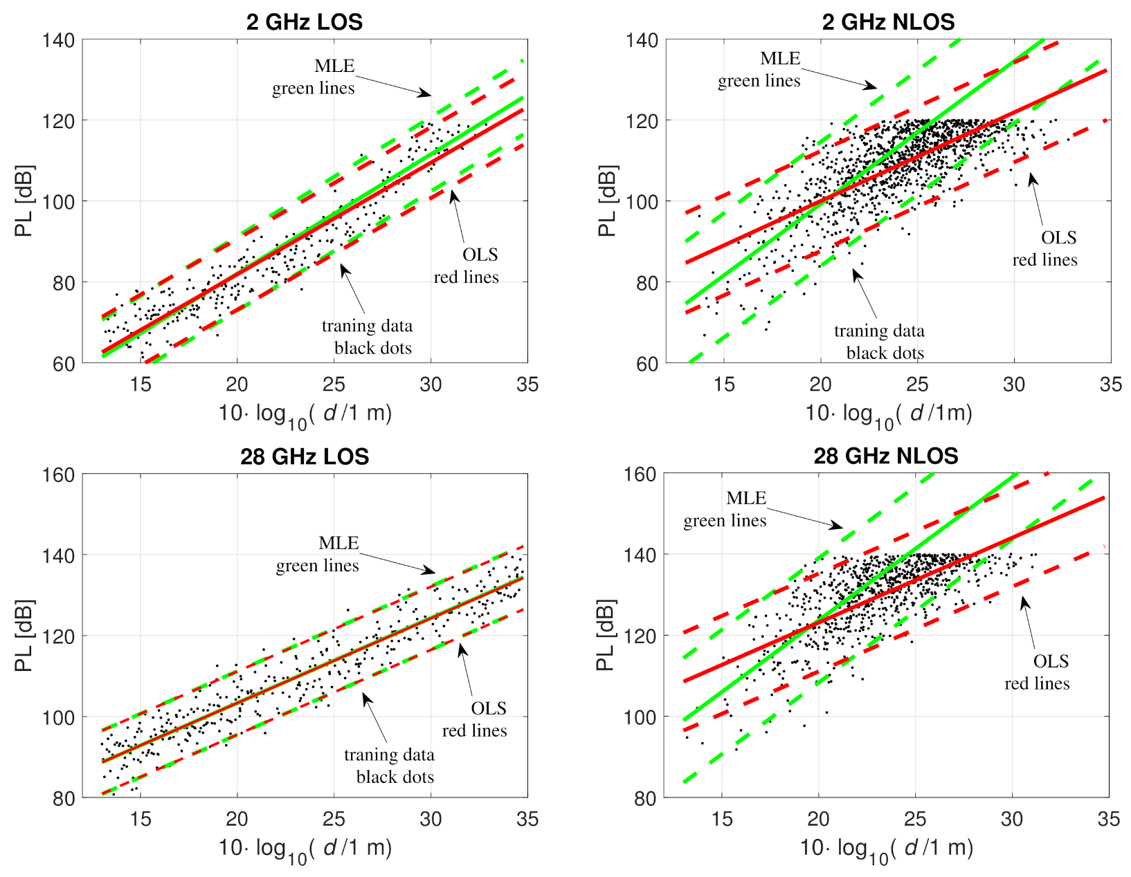
Figure 4.
Fitting the path loss model to the training data with OLS (green) and MLE (red); Example 3, 2 GHz LOS, 2 GHz NLOS, 28 GHz LOS, 28 GHz NLOS. Training data with under the noise threshold are shown with black dots, solid lines show , and the dash lines are .
Figure 4.
Fitting the path loss model to the training data with OLS (green) and MLE (red); Example 3, 2 GHz LOS, 2 GHz NLOS, 28 GHz LOS, 28 GHz NLOS. Training data with under the noise threshold are shown with black dots, solid lines show , and the dash lines are .
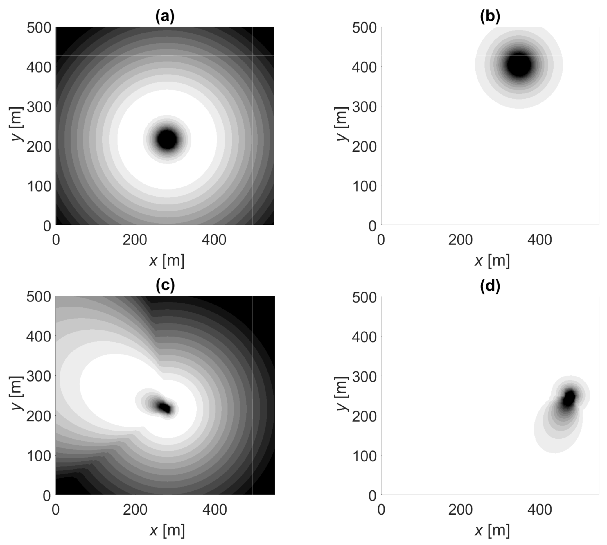
Figure 5.
Likelihood function illustrations: (a) measured PL and omnidirectional antenna, (b) censored PL and omnidirectional antenna, (c) measured PL and directive beam (), (d) censored PL and directive beam (). White is likely, gray is possible, and black is an unlikely location.
Figure 5.
Likelihood function illustrations: (a) measured PL and omnidirectional antenna, (b) censored PL and omnidirectional antenna, (c) measured PL and directive beam (), (d) censored PL and directive beam (). White is likely, gray is possible, and black is an unlikely location.
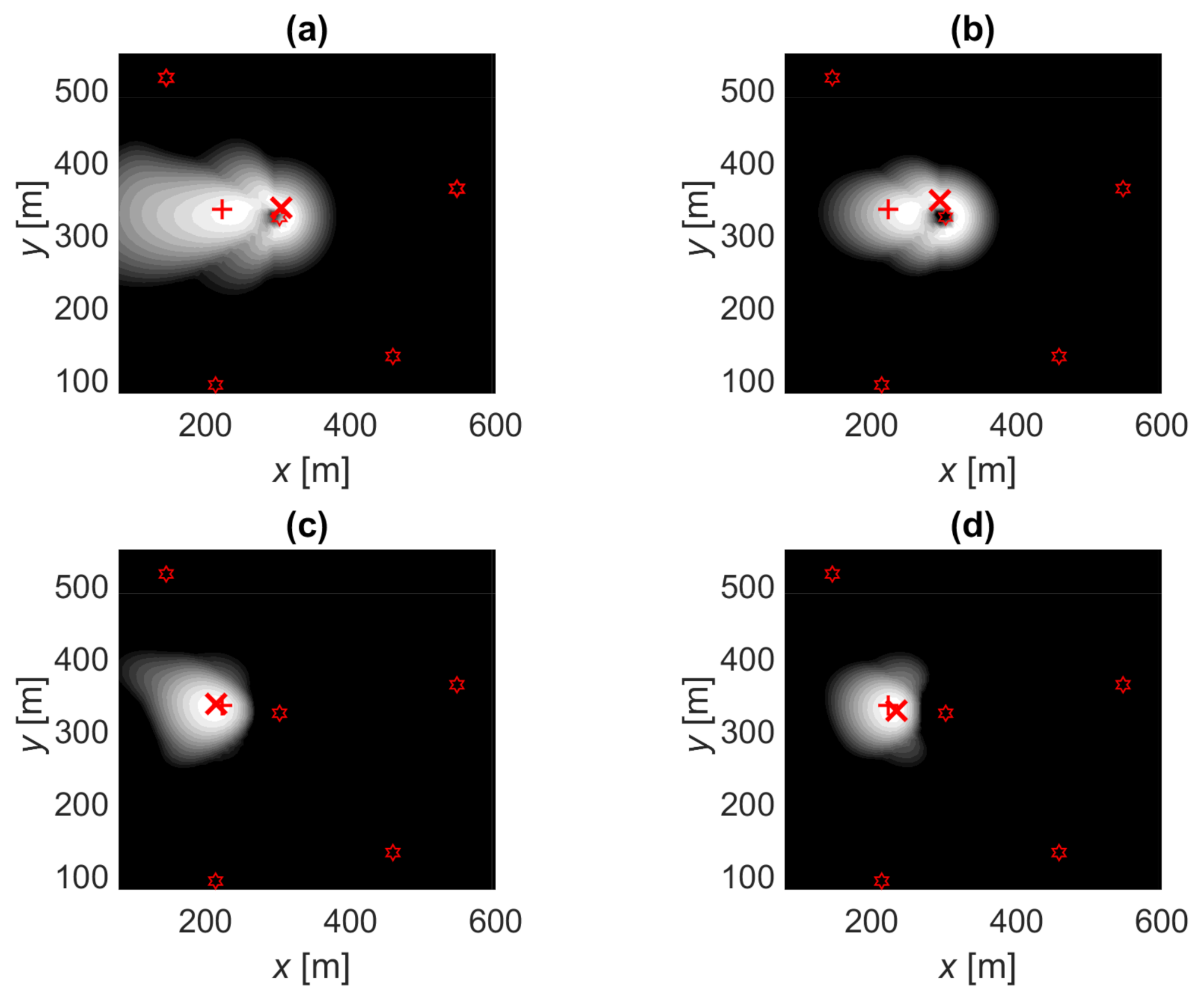
Figure 6.
Likelihood function illustrations: true location (+), position estimate (×), base stations (BSs; stars), contact with three BSs with directive antennas () at = (302,324), (547,363), and (146,516). White is likely, gray is possible, and black is an unlikely location.(a) OLS-OPT: ordinary least squares fitting and trilateration positioning. (b) MLE-OPT: Tobit MLE fitting and the ordinary trilateration positioning. (c) OLS-MLE: ordinary least squares fitting and the Tobit MLE positioning. (d) MLE-MLE: Tobit MLE fitting and the Tobit MLE positioning.
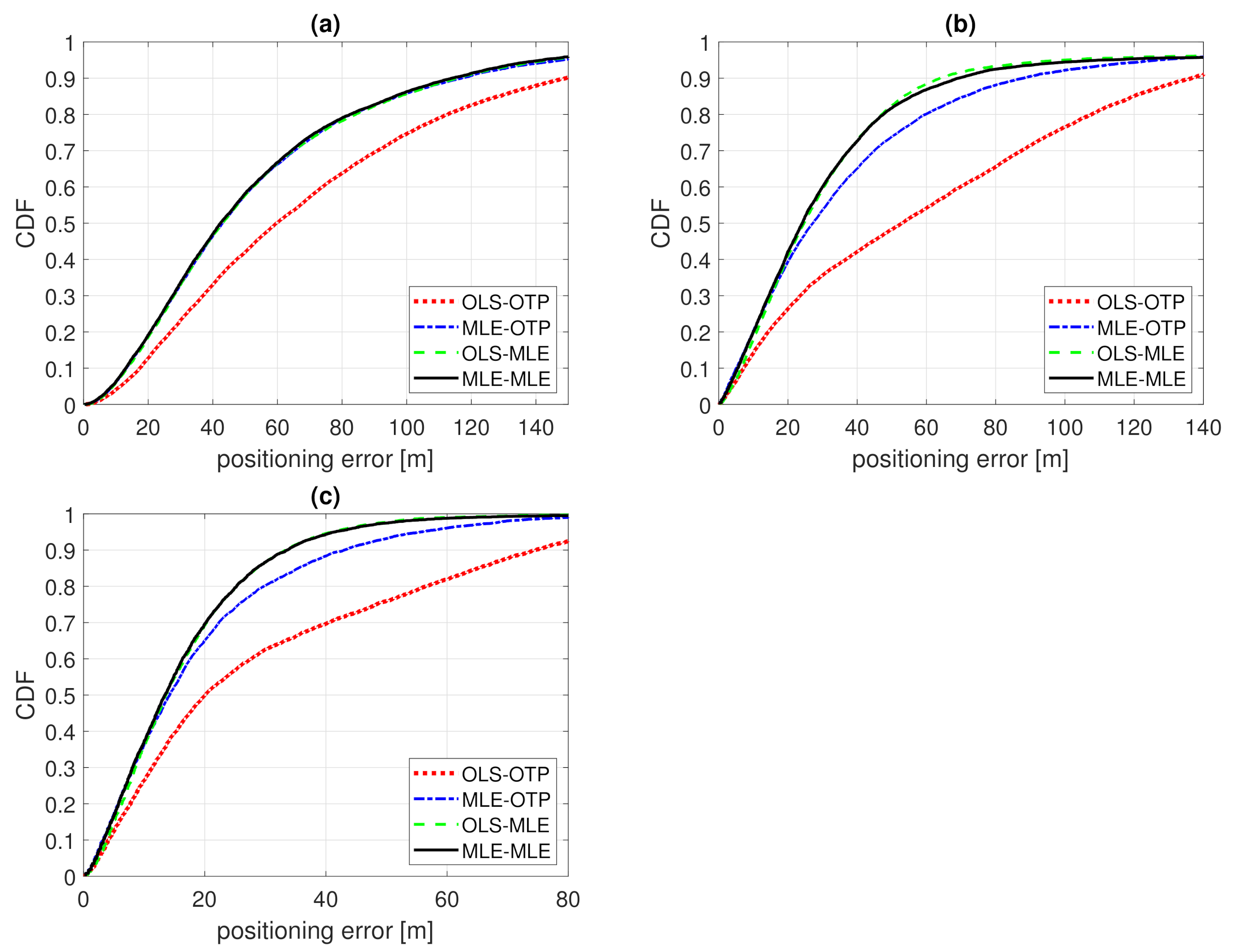
Figure 7.
CDF of positioning error of Example 1. Model fitting to training data with ordinary least squares (OLS-) or Tobit MLE fitting (MLE-) and positioning with either ordinary trilateration (-OTP) of Tobit MLE positioning (-MLE). (a) , ; (b) , ; (c) , .
Figure 7.
CDF of positioning error of Example 1. Model fitting to training data with ordinary least squares (OLS-) or Tobit MLE fitting (MLE-) and positioning with either ordinary trilateration (-OTP) of Tobit MLE positioning (-MLE). (a) , ; (b) , ; (c) , .
Figure 8.
CDF of positioning error of Example 2. Model fitting to training data with ordinary least squares (OLS-) or Tobit MLE fitting (MLE-) and positioning with either ordinary trilateration (-OTP) of Tobit MLE positioning (-MLE). (a) , ; (b) , ; (c) , .
Figure 8.
CDF of positioning error of Example 2. Model fitting to training data with ordinary least squares (OLS-) or Tobit MLE fitting (MLE-) and positioning with either ordinary trilateration (-OTP) of Tobit MLE positioning (-MLE). (a) , ; (b) , ; (c) , .
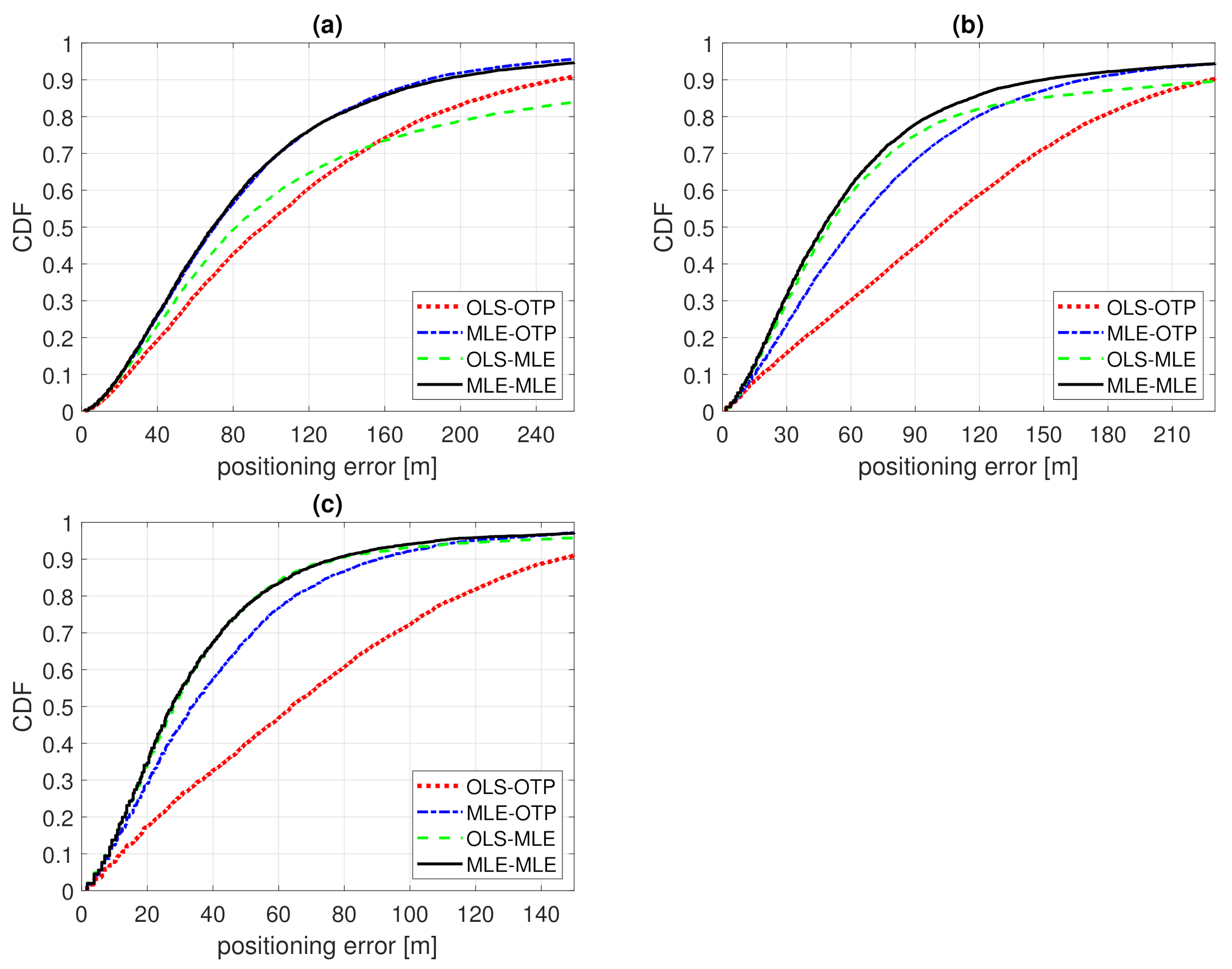
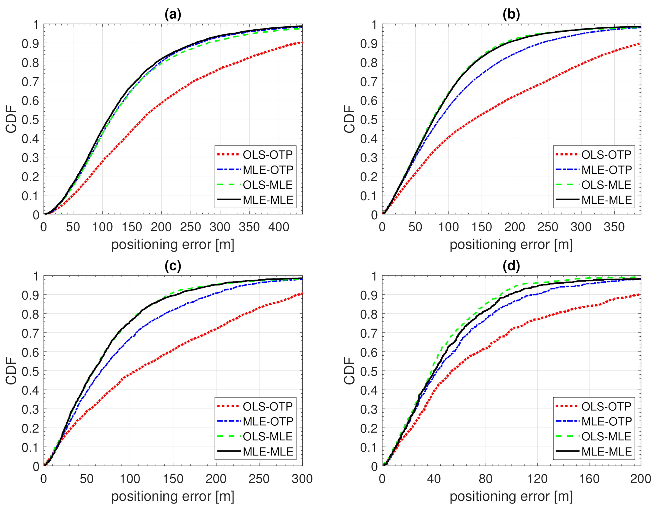
Figure 9.
CDF of positioning error of Example 3. Model fitting to training data with ordinary least squares (OLS-) or Tobit MLE fitting (MLE-) and positioning with either ordinary trilateration (-OTP) of Tobit MLE positioning (-MLE). (a) 2 GHz, , , (b) 2 GHz, , , (c) 28 GHz, , , (d) 28 GHz, , .
Figure 9.
CDF of positioning error of Example 3. Model fitting to training data with ordinary least squares (OLS-) or Tobit MLE fitting (MLE-) and positioning with either ordinary trilateration (-OTP) of Tobit MLE positioning (-MLE). (a) 2 GHz, , , (b) 2 GHz, , , (c) 28 GHz, , , (d) 28 GHz, , .
Table 1.
Fitted ordinary least squares (OLS) and maximum likelihood estimation (MLE) parameter estimates for Example 1 (, , ) and Example 2 (, , ).
Table 1.
Fitted ordinary least squares (OLS) and maximum likelihood estimation (MLE) parameter estimates for Example 1 (, , ) and Example 2 (, , ).
| | | | | |
|---|
| Example 1 | OLS | 2.5 | 83 | 5.8 |
| MLE | 4.0 | 60 | 7.0 |
| Example 2 | OLS | 1.3 | 63 | 5.6 |
| MLE | 2.2 | 51 | 7.6 |
Table 2.
Fitted OLS and MLE parameter estimates for Example 3 at 2 and 28 GHz.
Table 2.
Fitted OLS and MLE parameter estimates for Example 3 at 2 and 28 GHz.
| | | | | | |
|---|
| 2 GHz | LOS | OLS | 2.8 | 27 | 4.5 |
| MLE | 3.0 | 23 | 4.7 |
| NLOS | OLS | 2.2 | 56 | 6.3 |
| MLE | 3.5 | 29 | 7.8 |
| 28 GHz | LOS | OLS | 2.1 | 61 | 4.0 |
| MLE | 2.1 | 61 | 4.0 |
| NLOS | OLS | 2.1 | 81 | 6.2 |
| MLE | 3.5 | 53 | 7.8 |
Table 3.
Positioning error, in meters, 50th and 90th percentiles of Example 1. Base stations have omnidirectional () or directional antennas () and the average number of contacted BSs is 2, 3, or 5.
Table 3.
Positioning error, in meters, 50th and 90th percentiles of Example 1. Base stations have omnidirectional () or directional antennas () and the average number of contacted BSs is 2, 3, or 5.
| 2 | 3 | 5 | 2 | 3 | 5 |
| N | 1 | 1 | 1 | 8 | 8 | 8 |
| 159 | 129 | 100 | 245 | 199 | 154 |
| | 50% | 90% | 50% | 90% | 50% | 90% | 50% | 90% | 50% | 90% | 50% | 90% |
| OLS-OTP | 60 | 149 | 43 | 108 | 29 | 77 | 53 | 137 | 34 | 101 | 20 | 74 |
| MLE-OTP | 43 | 117 | 29 | 72 | 20 | 48 | 27 | 88 | 19 | 59 | 14 | 43 |
| OLS-MLE | 43 | 116 | 28 | 72 | 20 | 44 | 25 | 64 | 19 | 44 | 14 | 33 |
| MLE-MLE | 42 | 114 | 28 | 69 | 19 | 43 | 24 | 69 | 18 | 45 | 13 | 34 |
Table 4.
Positioning error, in meters, 50th and 90th percentiles of Example 2. Base stations have omnidirectional () or directional antennas () and the average number of contacted BSs is 5 or 10.
Table 4.
Positioning error, in meters, 50th and 90th percentiles of Example 2. Base stations have omnidirectional () or directional antennas () and the average number of contacted BSs is 5 or 10.
| 5 | 10 | 5 | 10 |
| N | 1 | 1 | 8 | 8 |
| 459 | 325 | 515 | 420 |
| | 50% | 90% | 50% | 90% | 50% | 90% | 50% | 90% |
| OLS-OTP | 96 | 251 | 66 | 164 | 101 | 228 | 64 | 146 |
| MLE-OTP | 71 | 182 | 46 | 105 | 61 | 168 | 34 | 90 |
| OLS-MLE | 82 | 352 | 49 | 259 | 49 | 236 | 28 | 78 |
| MLE-MLE | 69 | 190 | 45 | 106 | 47 | 149 | 28 | 77 |
Table 5.
Positioning error, in meters, 50th and 90th percentiles of Example 3 (2 GHz) with variable noise threshold level . Base stations have omni-directional (N = 1) BS antennas and the average number of contacted BSs is 5.
Table 5.
Positioning error, in meters, 50th and 90th percentiles of Example 3 (2 GHz) with variable noise threshold level . Base stations have omni-directional (N = 1) BS antennas and the average number of contacted BSs is 5.
| 120 dB | 125 dB | 130 dB | 135 dB | 140 dB |
| 459 m | 623 m | 846 m | 1164 m | 1600 m |
| | 50% | 90% | 50% | 90% | 50% | 90% | 50% | 90% | 50% | 90% |
| OLS-OTP | 168 | 434 | 234 | 595 | 316 | 801 | 425 | 1063 | 554 | 1396 |
| MLE-OTP | 114 | 265 | 158 | 377 | 218 | 525 | 302 | 716 | 416 | 987 |
| OLS-MLE | 114 | 279 | 154 | 361 | 206 | 500 | 283 | 683 | 395 | 950 |
| MLE-MLE | 110 | 259 | 150 | 351 | 203 | 485 | 283 | 674 | 391 | 929 |
Table 6.
Positioning error, in meters, 50th and 90th percentiles of Example 3 (28 GHz) with variable LOS detection probability in the positioning phase . Base stations have directional antennas () and the average number of contacted BSs is 10.
Table 6.
Positioning error, in meters, 50th and 90th percentiles of Example 3 (28 GHz) with variable LOS detection probability in the positioning phase . Base stations have directional antennas () and the average number of contacted BSs is 10.
| 100 | 95 | 90 | 85 | 80 |
| | 50% | 90% | 50% | 90% | 50% | 90% | 50% | 90% | 50% | 90% |
| OLS-OTP | 54 | 198 | 64 | 258 | 78 | 357 | 98 | 458 | 126 | 548 |
| MLE-OTP | 42 | 117 | 50 | 183 | 61 | 270 | 74 | 341 | 96 | 436 |
| OLS-MLE | 38 | 92 | 41 | 126 | 47 | 196 | 55 | 288 | 66 | 403 |
| MLE-MLE | 40 | 98 | 45 | 148 | 53 | 244 | 63 | 329 | 78 | 421 |
Table 7.
Positioning error, in meters, 50th and 90th percentiles of Example 3 (2 GHz). Base stations have omnidirectional () or directional antennas () and the average number of contacted BSs is 5 or 10.
Table 7.
Positioning error, in meters, 50th and 90th percentiles of Example 3 (2 GHz). Base stations have omnidirectional () or directional antennas () and the average number of contacted BSs is 5 or 10.
| 5 | 10 | 5 | 10 |
| N | 1 | 1 | 8 | 8 |
| 253 | 207 | 160 | 113 |
| | 50% | 90% | 50% | 90% | 50% | 90% | 50% | 90% |
| OLS-OTP | 168 | 434 | 104 | 273 | 139 | 392 | 73 | 250 |
| MLE-OTP | 114 | 265 | 73 | 162 | 86 | 240 | 57 | 156 |
| OLS-MLE | 114 | 279 | 73 | 158 | 76 | 184 | 50 | 119 |
| MLE-MLE | 110 | 259 | 70 | 150 | 77 | 188 | 53 | 132 |
Table 8.
Positioning error, in meters, 50th and 90th percentiles of Example 3 (28 GHz). Base stations have omnidirectional () or directional antennas () and the average number of contacted BSs is 5 or 10.
Table 8.
Positioning error, in meters, 50th and 90th percentiles of Example 3 (28 GHz). Base stations have omnidirectional () or directional antennas () and the average number of contacted BSs is 5 or 10.
| 5 | 10 | 5 | 10 |
| N | 1 | 1 | 8 | 8 |
| 390 | 276 | 565 | 399 |
| | 50% | 90% | 50% | 90% | 50% | 90% | 50% | 90% |
| OLS-OTP | 158 | 394 | 97 | 250 | 107 | 295 | 54 | 198 |
| MLE-OTP | 110 | 258 | 68 | 160 | 66 | 195 | 42 | 117 |
| OLS-MLE | 109 | 275 | 66 | 146 | 59 | 144 | 38 | 92 |
| MLE-MLE | 107 | 253 | 64 | 144 | 58 | 154 | 40 | 98 |


