
Ion Current Sensor for Gas Turbine Condition Dynamical Monitoring: Modeling and Characterization

 ,
,  , , ,
, , ,
Abstract
:1. Introduction
2. Measurement System Model
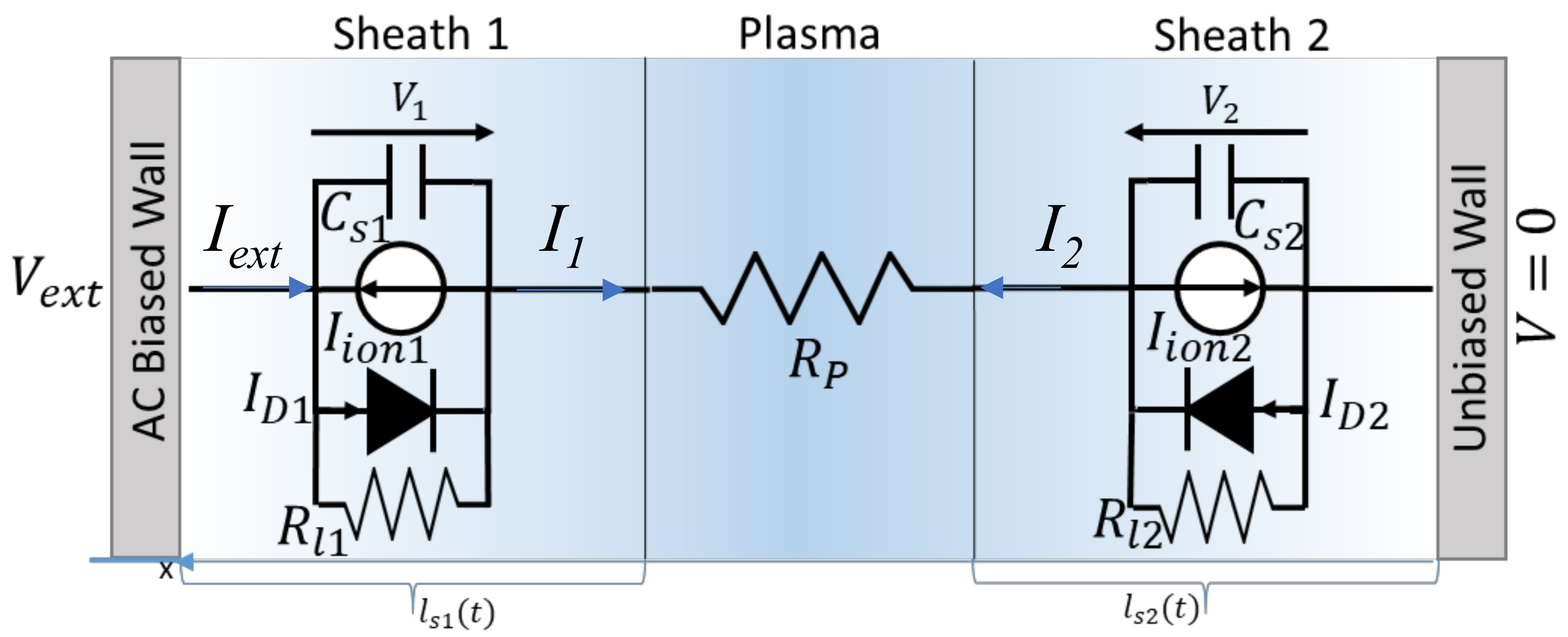
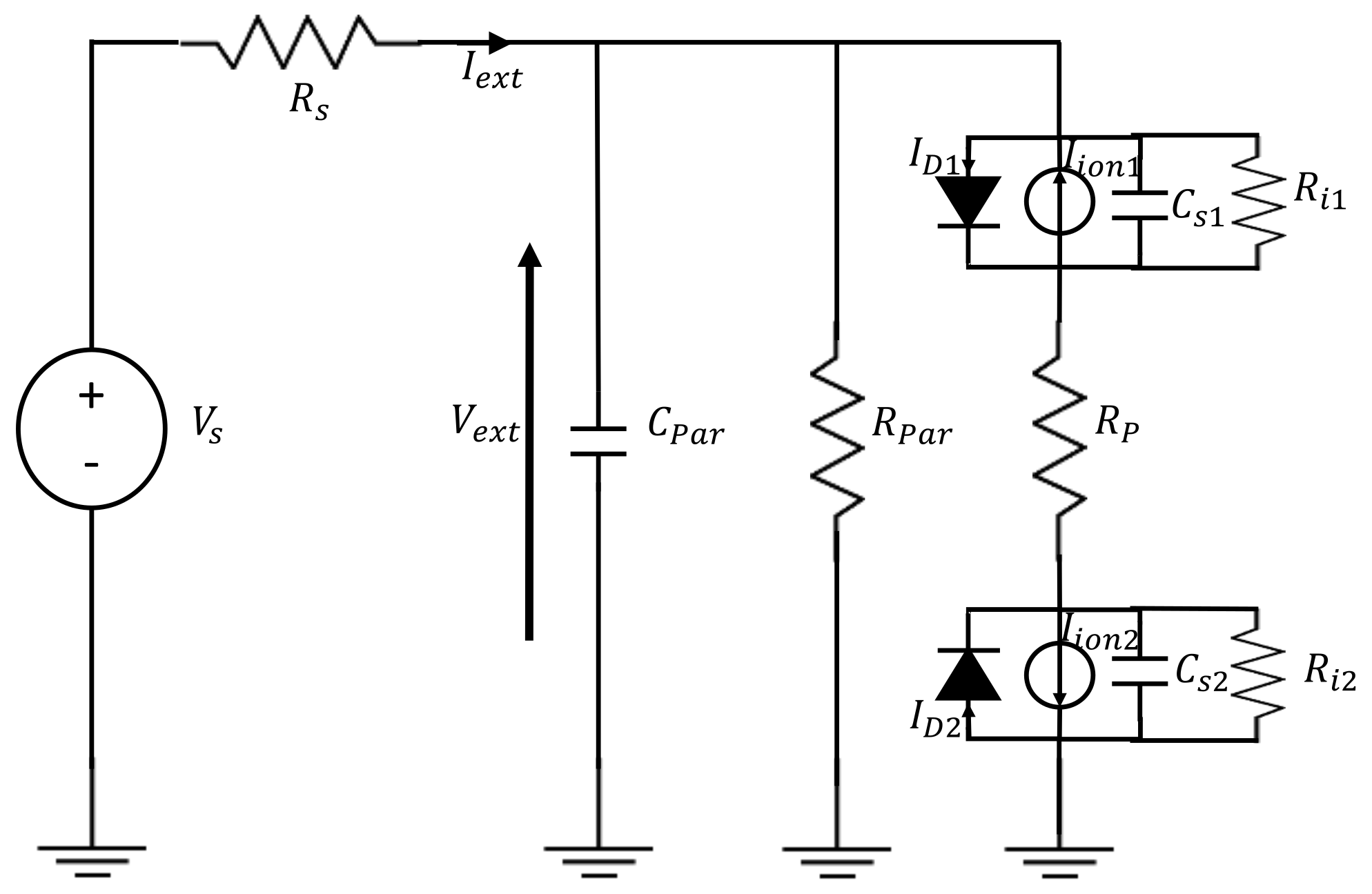
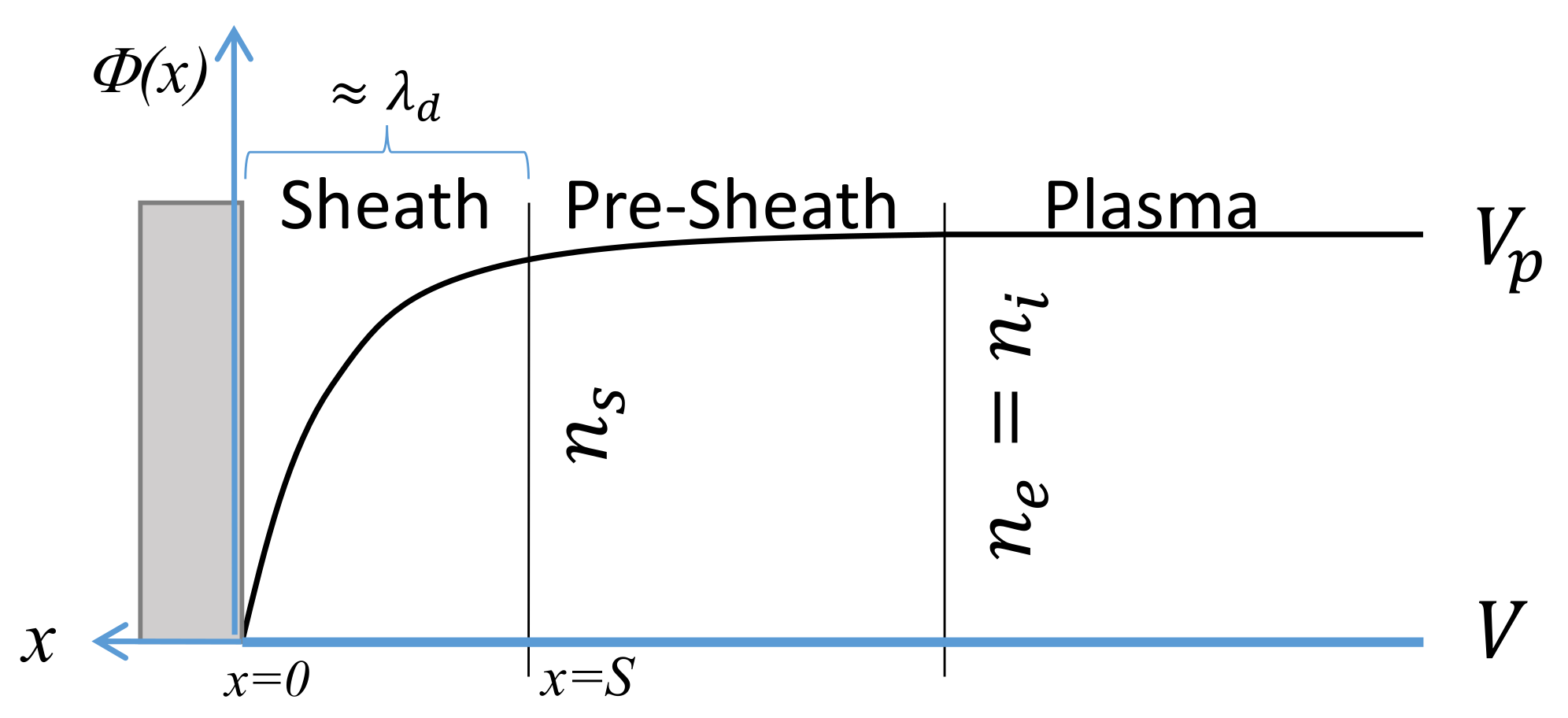
2.1. Sensor Model
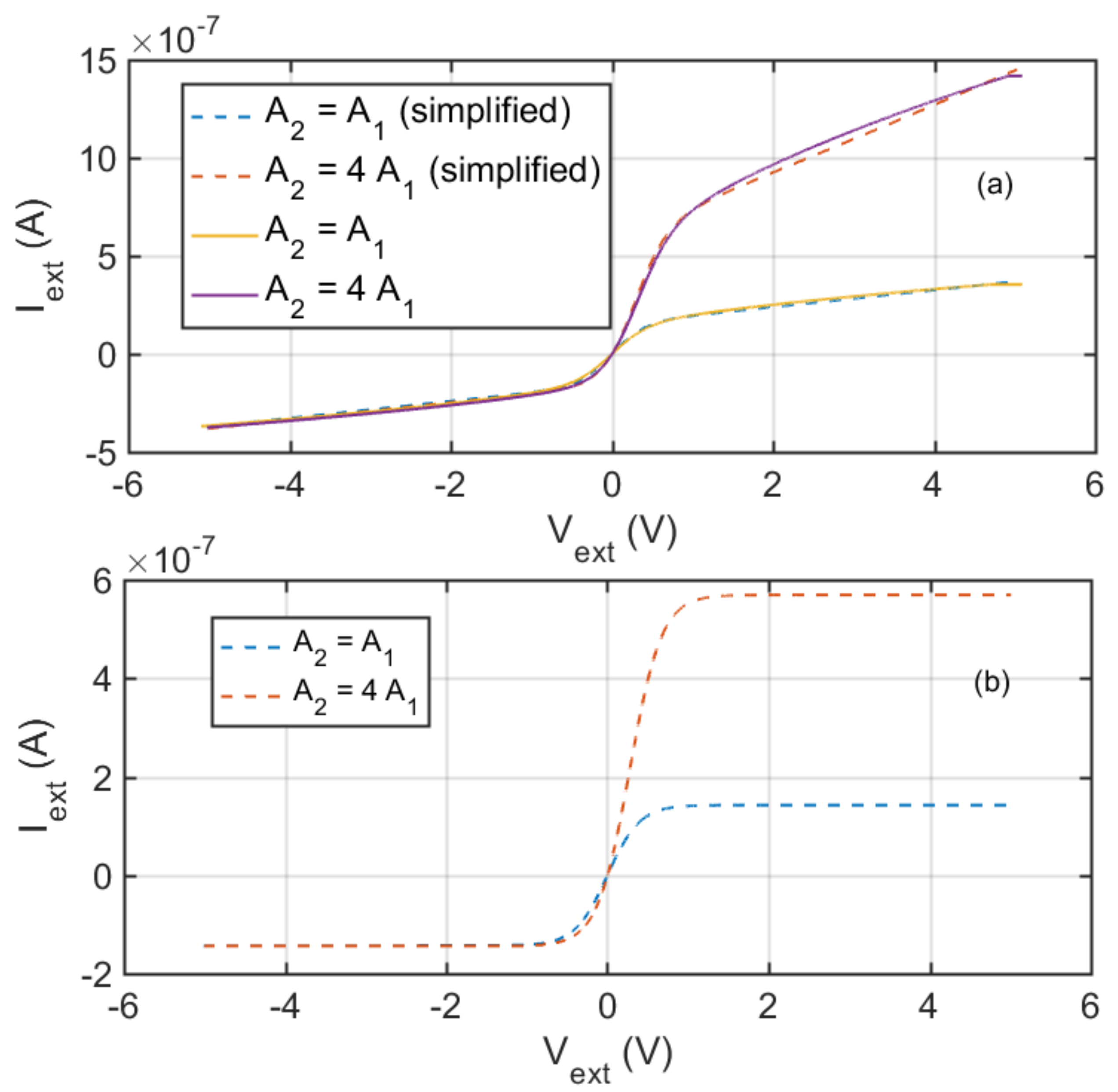
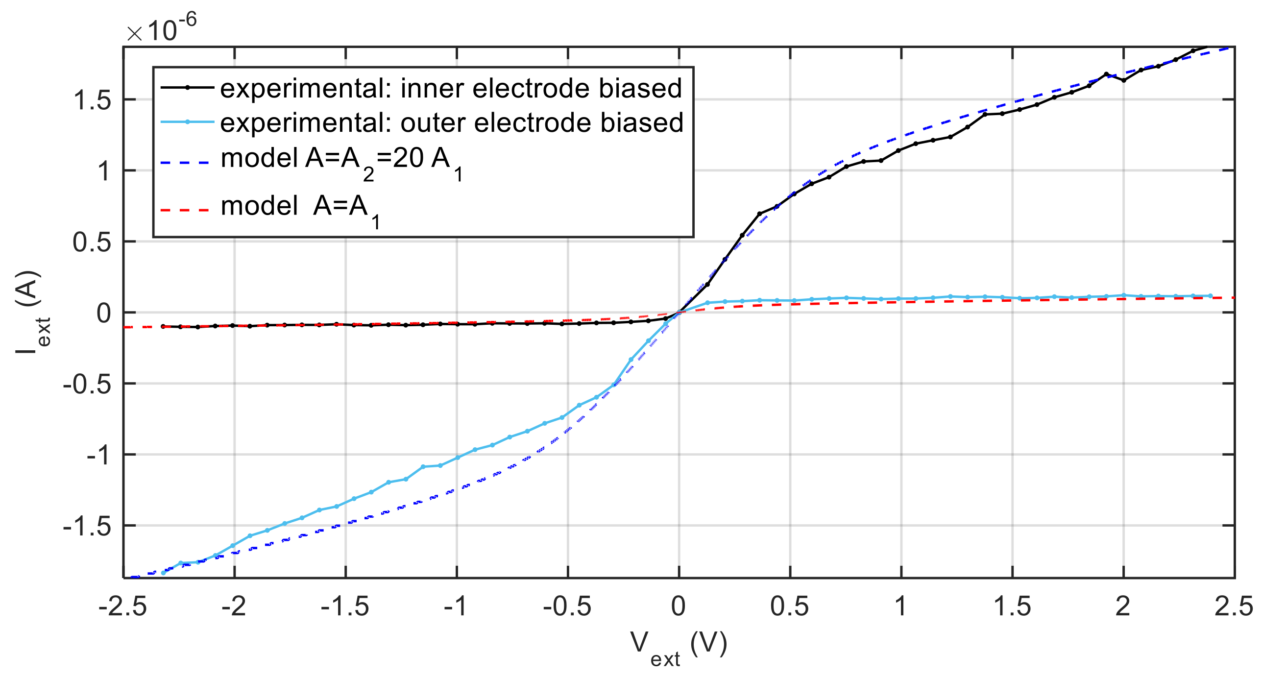
2.2. Response of the Ion Sensor to Small Dynamic Signals
3. Experimental Setup
3.1. Measurement Technique
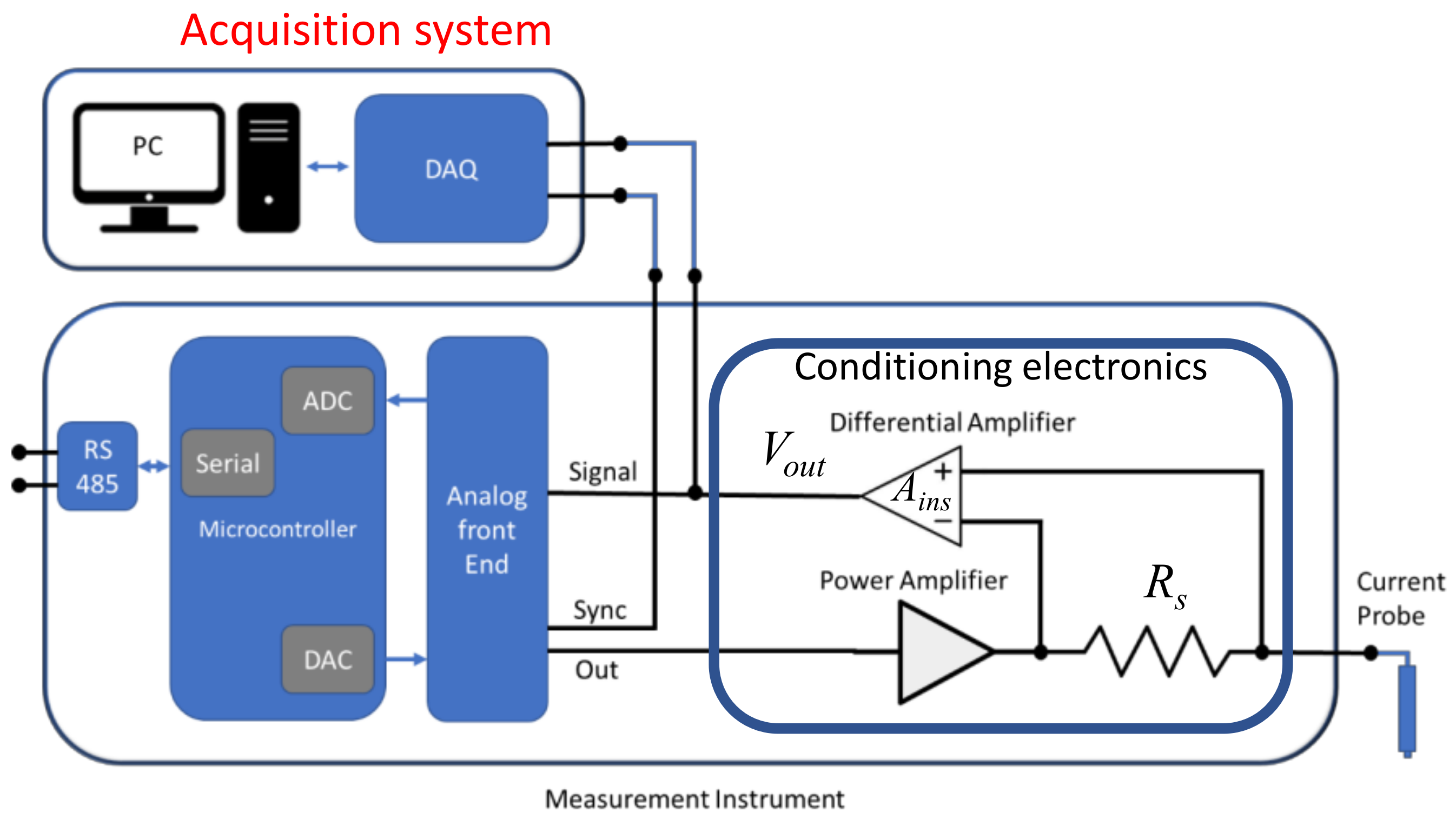
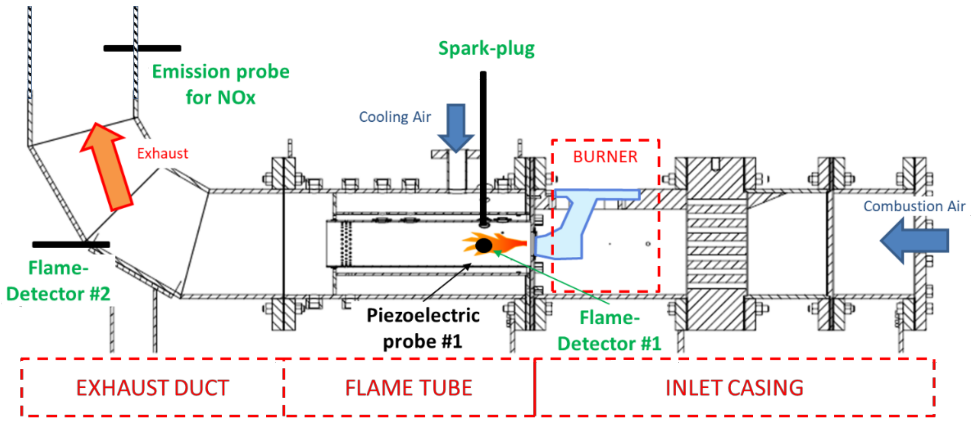
3.2. Measurement Setup
4. Experimental Results
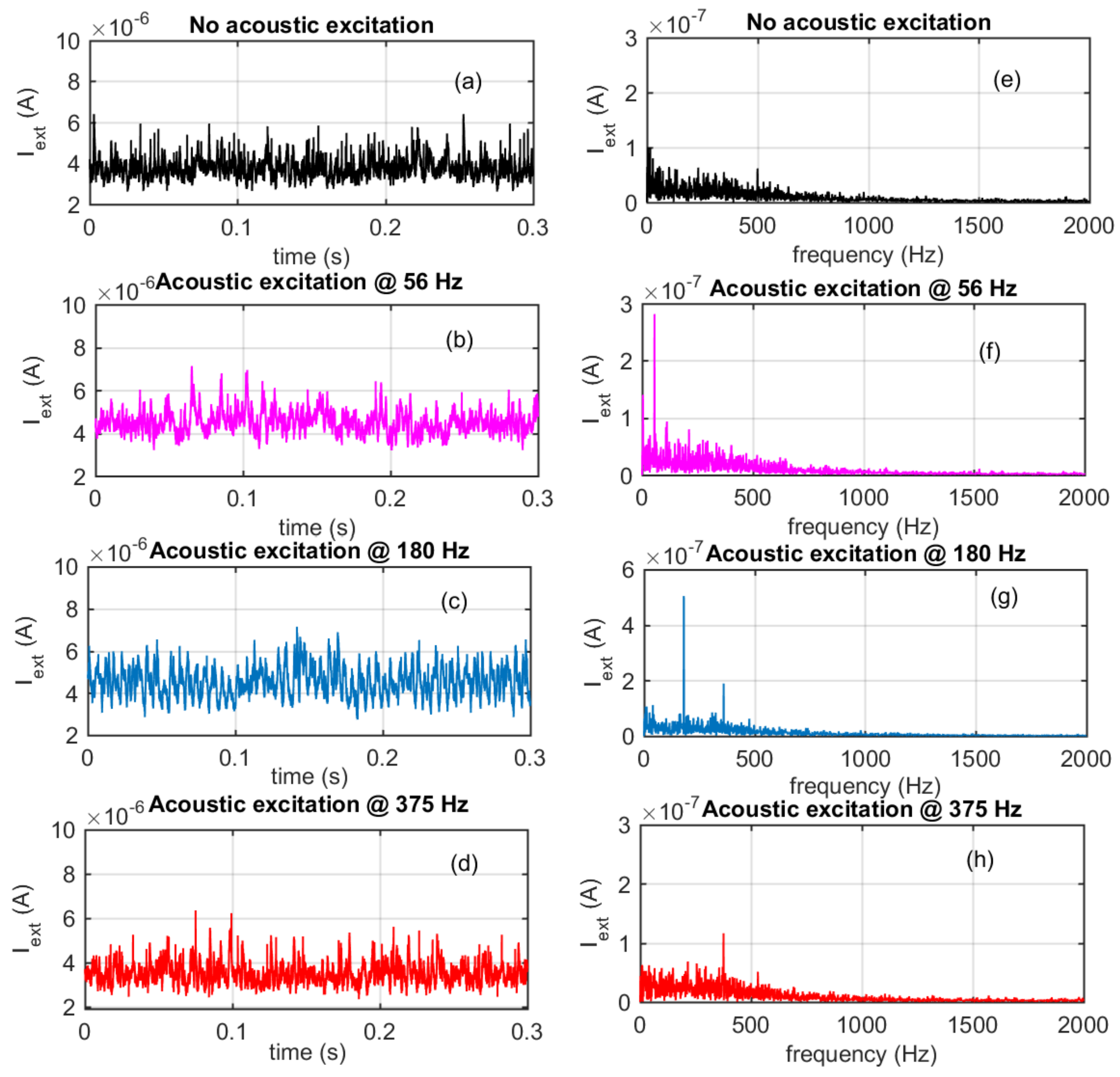
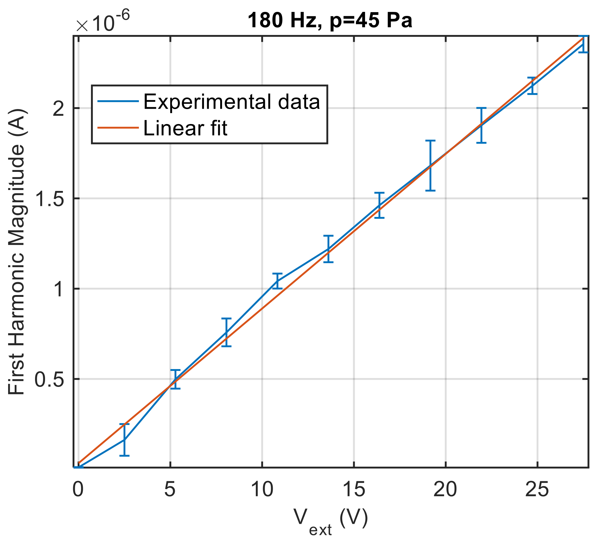
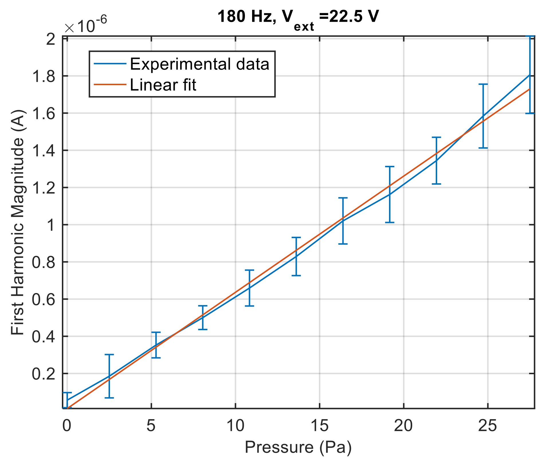
4.1. Laboratory Tests
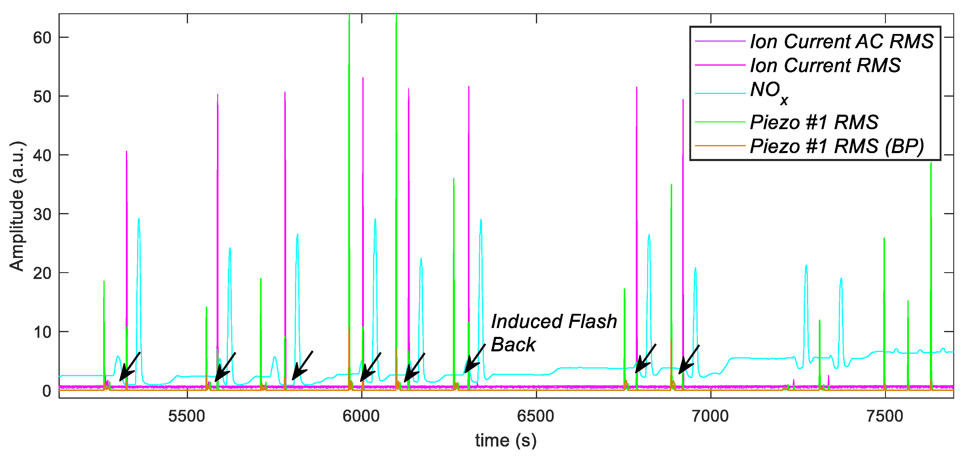
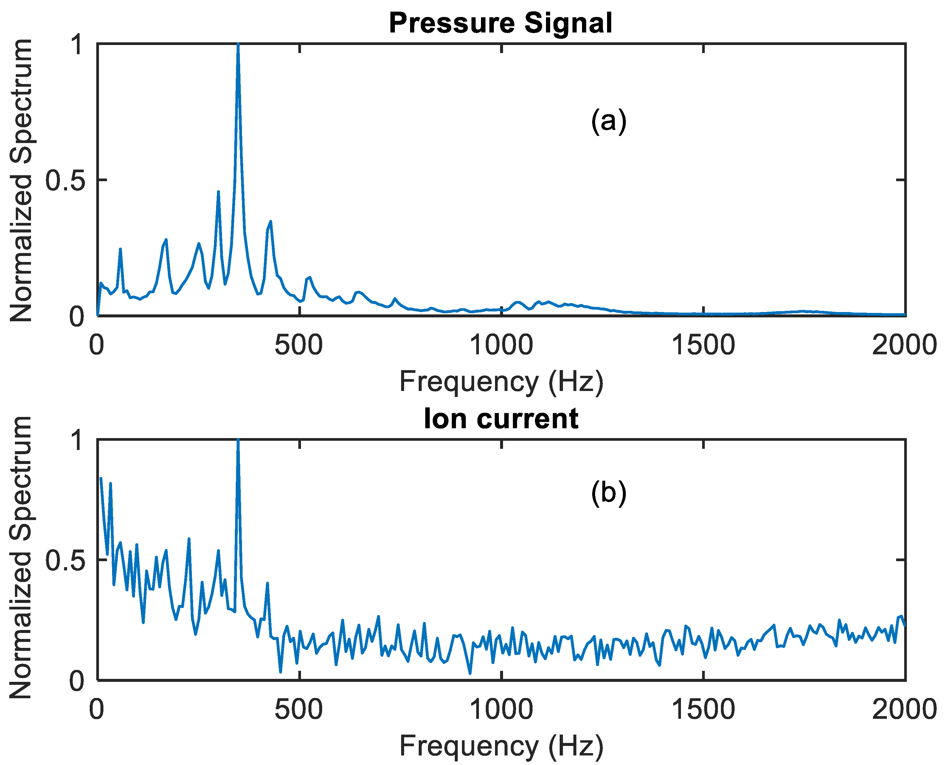
4.2. In Field Measurements
5. Conclusions
Author Contributions
Funding
Institutional Review Board Statement
Informed Consent Statement
Conflicts of Interest
Appendix A. Derivation of Equation (1)

References
- Griebel, P.; Boschek, E.; Jansohn, P. Lean Blowout Limits and NOx Emissions of Turbulent, Lean Premixed, Hydrogen-Enriched Methane/Air Flames at High Pressure. J. Eng. Gas Turbines Power 2007, 129, 404–410. [Google Scholar] [CrossRef]
- Rosfjord, T.J.; Cohen, J.M. Evaluation of the transient operation of advanced gas turbine combustors. J. Propuls. Power 1995, 11, 497–504. [Google Scholar] [CrossRef]
- Lieuwen, T.; McManus, K. That Elusive Hum. Mech. Eng. 2002, 124, 53–55. [Google Scholar] [CrossRef] [Green Version]
- Caraeni, M.; Devaki, R.; Aroni, M.; Oswald, M.; Srikanth, K.; Caraeni, D. Efficient Acoustic Modal Analysis for Industrial CFD. In Proceedings of the 47th AIAA Aerospace Sciences Meeting Including the New Horizons Forum and Aerospace Session: AA-10, Orlando, FL, USA, 5–8 January 2009. [Google Scholar]
- Zubrilin, I.A.; Gurakov, N.I.; Matveev, S. Modeling of natural acoustic frequencies of a gas-turbine plant combustion chamber. Therm. Eng. 2017, 64, 372–378. [Google Scholar] [CrossRef]
- Nair, S.; Rajaram, R.; Meyers, A.; Lieuwen, T.; Tozzi, L.; Benson, K. Acoustic and Ion Sensing of Lean Blowout in an Aircraft Combustor Simulator. In Proceedings of the 43rd AIAA Aerospace Sciences Session: PC-9, Reno, NV, USA, 10–13 January 2005. [Google Scholar]
- Zinn, B. Real-Time Control of Lean Blowout in a Turbine Engine for Minimizing No (x) Emissions; Georgia Institute of Technology, School of Aerospace: Atlanta, GA, USA, 2004. [Google Scholar]
- Ruan, C.; Chen, F.; Cai, W.; Qian, Y.; Yu, L.; Lu, X. Principles of non-intrusive diagnostic techniques and their applications for fundamental studies of combustion instabilities in gas turbine combustors: A brief review. Aerosp. Sci. Technol. 2019, 84, 585–603. [Google Scholar] [CrossRef]
- Cabot, G.; Vauchelles, D.; Taupin, B.; Boukhalfa, A. Experimental study of lean premixed turbulent combustion in a scale gas turbine chamber. Exp. Therm. Fluid Sci. 2004, 28, 683–690. [Google Scholar] [CrossRef]
- Addabbo, T.; Fort, A.; Mugnaini, M.; Parri, L.; Vignoli, V.; Allegorico, M.; Ruggiero, M.; Cioncolini, S. Ion Sensor-Based Measurement Systems: Application to Combustion Monitoring in Gas Turbines. IEEE Trans. Instrum. Meas. 2019, 69, 1474–1483. [Google Scholar] [CrossRef]
- Wollgarten, J.C.; Zarzalis, N.; Turrini, F.; Peschiulli, A. Experimental investigations of ion current in liquid-fuelled gas turbine combustors. Int. J. Spray Combust. Dyn. 2017, 9, 172–185. [Google Scholar] [CrossRef]
- Martinez-Garcia, M.; Zhang, Y.; Suzuki, K.; Zhang, Y.-D. Deep Recurrent Entropy Adaptive Model for System Reliability Monitoring. IEEE Trans. Ind. Inform. 2021, 17, 839–848. [Google Scholar] [CrossRef]
- Martinez-Garcia, M.; Zhang, Y.; Wan, J.; McGinty, J. Visually interpretable profile extraction with an autoencoder for health monitoring of industrial systems. In Proceedings of the 2019 IEEE 4th International Conference on Advanced Robotics and Mechatronics (ICARM), Osaka, Japan, 3–5 July 2019. [Google Scholar]
- Ben Rahmoune, M.; Hafaifa, A.; Kouzou, A.; Chen, X.; Chaibet, A. Gas turbine monitoring using neural network dynamic nonlinear autoregressive with external exogenous input modelling. Math. Comput. Simul. 2021, 179, 23–47. [Google Scholar] [CrossRef]
- Djeddi, C.; Hafaifa, A.; Iratni, A.; Hadroug, N.; Chen, X. Robust diagnosis with high protection to gas turbine failures identification based on a fuzzy neuro inference monitoring approach. J. Manuf. Syst. 2021, 59, 190–213. [Google Scholar] [CrossRef]
- Zaccaria, V.; Rahman, M.; Aslanidou, I.; Kyprianidis, K. A Review of Information Fusion Methods for Gas Turbine Diagnostics. Sustainability 2019, 11, 6202. [Google Scholar] [CrossRef] [Green Version]
- Salilew, W.M.; Karim, Z.A.A.; Baheta, A.T. Review on gas turbine condition based diagnosis method. Mater. Today Proc. 2021. [Google Scholar] [CrossRef]
- Wen, Z.; Hou, J.; Atkin, J. A review of electrostatic monitoring technology: The state of the art and future research directions. Prog. Aerosp. Sci. 2017, 94, 1–11. [Google Scholar] [CrossRef] [Green Version]
- Addabbo, T.; Fort, A.; Mugnaini, M.; Panzardi, E.; Vignoli, V. Measurement System Based on Electrostatic Sensors to Detect Moving Charged Debris With Planar-Isotropic Accuracy. IEEE Trans. Instrum. Meas. 2018, 68, 837–844. [Google Scholar] [CrossRef]
- Addabbo, T.; Fort, A.; Mugnaini, M.; Panzardi, E.; Vignoli, V. A Smart Measurement System With Improved Low-Frequency Response to Detect Moving Charged Debris. IEEE Trans. Instrum. Meas. 2016, 65, 1874–1883. [Google Scholar] [CrossRef]
- Addabbo, T.; Fort, A.; Mugnaini, M.; Panzardi, E.; Rocchi, S.; Vignoli, V. Automated testing and characterization of electrostatic measurement systems for the condition monitoring of turbo machinery. In Proceedings of the 2016 IEEE Metrology for Aerospace (MetroAeroSpace), Florence, Italy, 22–23 June 2016; pp. 271–275. [Google Scholar] [CrossRef]
- Gamalath, K.W.; Samarakoon, A. Modeling of Planar Plasma Diode. Int. Lett. Chem. Phys. Astron. 2013, 13, 220–242. [Google Scholar] [CrossRef] [Green Version]
- Jin, S.; Poulos, M.J.; Van Compernolle, B.; Morales, G.J. Plasma flows generated by an annular thermionic cathode in a large magnetized plasma. Phys. Plasmas 2019, 26, 022105. [Google Scholar] [CrossRef] [Green Version]
- Sierra, F.Z.; Kubiak, J.; González, G.; Urquiza, G. Prediction of temperature front in a gas turbine combustion chamber. Appl. Therm. Eng. 2005, 25, 1127–1140. [Google Scholar] [CrossRef]
- Timmons, R.B.R.S. The Application of Plasmas to Chemical Processing; MIT Press: Cambridge, MA, USA, 1967. [Google Scholar]
- Goldston, R.J. Introduction to Plasma Physics; CRC Press: Boca Raton, FL, USA, 2020. [Google Scholar]
- Callen, J.D. Fundamentals of Plasma Physics; Online Book: Madison, WI, USA, 2006. [Google Scholar]
- Aarts, R.M.; Janssen, A.J.E.M. Comparing sound radiation from a loudspeaker with that from a flexible spherical cap on a rigid sphere. J. Audio Eng. Soc. 2011, 59, 201–212. [Google Scholar]
- Stangeby, P.C. The Plasma Sheath. Physics of Plasma-Wall Interactions in Controlled Fusion; Springer: Berlin/Heidelberg, Germany, 1986; pp. 41–97. [Google Scholar]
- Xu, K.G. Plasma sheath behavior and ionic wind effect in electric field modified flames. Combust. Flame 2013, 161, 1678–1686. [Google Scholar] [CrossRef]
- Goodings, J.M.; Guo, J.; Hayhurst, A.N.; Taylor, S.G. Current–voltage characteristics in a flame plasma: Analysis for positive and negative ions, with applications. Int. J. Mass Spectrom. 2001, 206, 137–151. [Google Scholar] [CrossRef]
- Ostretsov, I.N.; Petrosov, V.A.; Porotnikov, A.A.; Rodnevich, B.B. Equation for thermionic emission in a plasma. J. Appl. Mech. Tech. Phys. 1974, 13, 296–300. [Google Scholar] [CrossRef]


| Parallel Capacitance | Diodes 1 and 2 | Constant Current Generators 1 and 2 | Loss Resistances | Gas Path Resistance | |
|---|---|---|---|---|---|
j = 1, 2 | ; ; | If | |||
j = 1, 2 | ; ; |
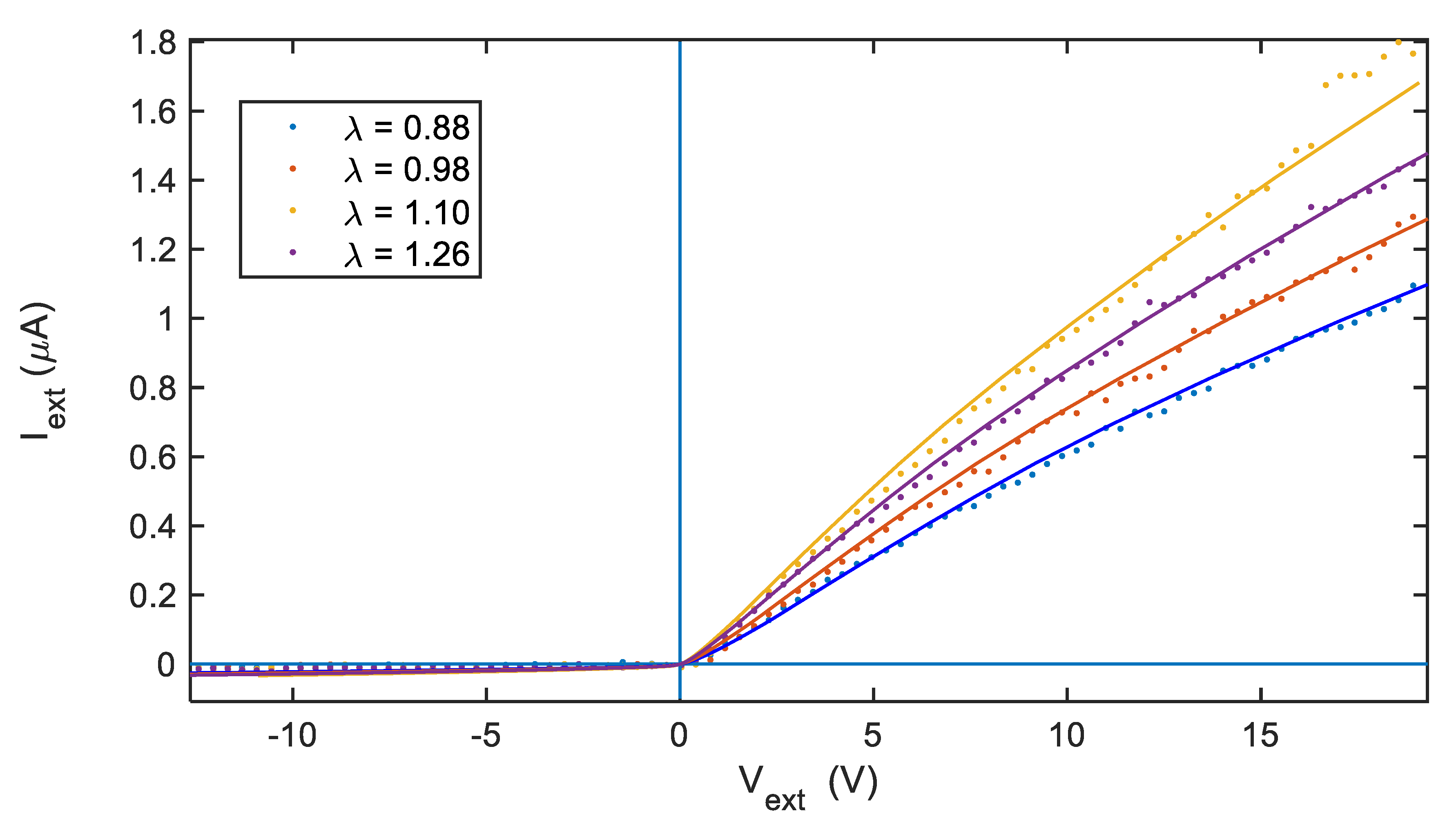
| Air-Fuel Equivalence Ratio (λ) | ns (m−3) | μe (m2/ (V s)) | Te (K) |
|---|---|---|---|
| 0.88 | 1.15 × 10¹³ | 80 | 2000 |
| 0.98 | 1.35 × 10¹³ | 80 | 1500 |
| 1.10 | 1.78 × 10¹³ | 80 | 1000 |
| 1.26 | 1.55 × 10¹³ | 80 | 1000 |
Publisher’s Note: MDPI stays neutral with regard to jurisdictional claims in published maps and institutional affiliations. |
© 2021 by the authors. Licensee MDPI, Basel, Switzerland. This article is an open access article distributed under the terms and conditions of the Creative Commons Attribution (CC BY) license (https://creativecommons.org/licenses/by/4.0/).
Share and Cite
Addabbo, T.; Fort, A.; Landi, E.; Mugnaini, M.; Parri, L.; Vignoli, V.; Zucca, A.; Romano, C. Ion Current Sensor for Gas Turbine Condition Dynamical Monitoring: Modeling and Characterization. Sensors 2021, 21, 6944. https://doi.org/10.3390/s21206944
Addabbo T, Fort A, Landi E, Mugnaini M, Parri L, Vignoli V, Zucca A, Romano C. Ion Current Sensor for Gas Turbine Condition Dynamical Monitoring: Modeling and Characterization. Sensors. 2021; 21(20):6944. https://doi.org/10.3390/s21206944
Chicago/Turabian StyleAddabbo, Tommaso, Ada Fort, Elia Landi, Marco Mugnaini, Lorenzo Parri, Valerio Vignoli, Alessandro Zucca, and Christian Romano. 2021. "Ion Current Sensor for Gas Turbine Condition Dynamical Monitoring: Modeling and Characterization" Sensors 21, no. 20: 6944. https://doi.org/10.3390/s21206944