
The Experimental Verification of Direct-Write Silver Conductive Grid and ARIMA Time Series Analysis for Crack Propagation

 , , , , and
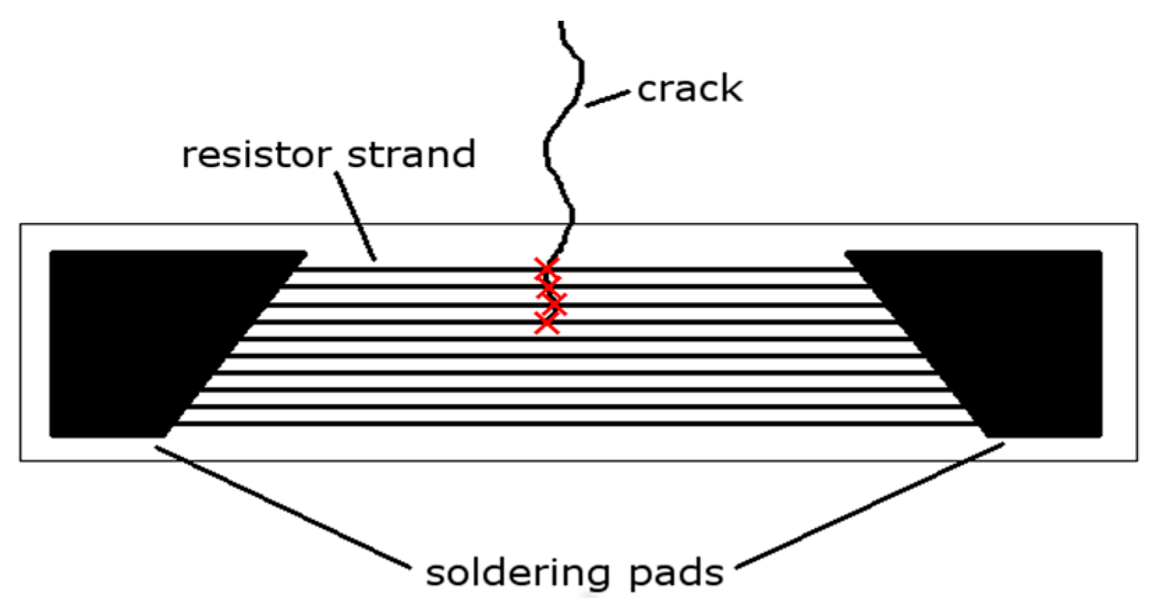
Abstract
:1. Introduction
- Demands for reductions in maintenance costs (reductions in inspection times, reductions in inspection efforts, improvements in inspection quality, etc.);
- Demands for certifiable SHM systems that enable underwriting new aircraft materials and designs;
- Demands for improvements in operational management, affordability, and performance.
1.1. The State-of-the-Art
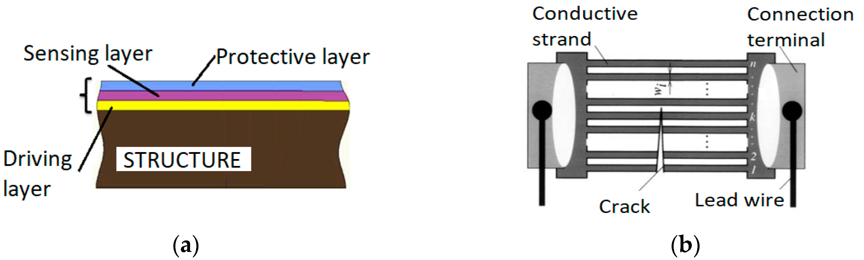
1.2. Customized Resistive Crack Propagation Sensors
2. Materials and Methods
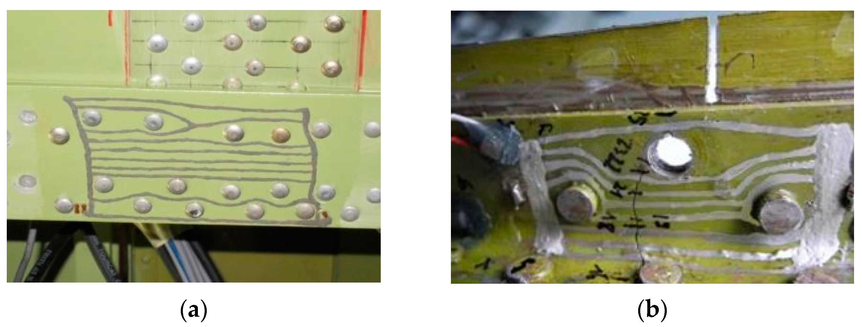
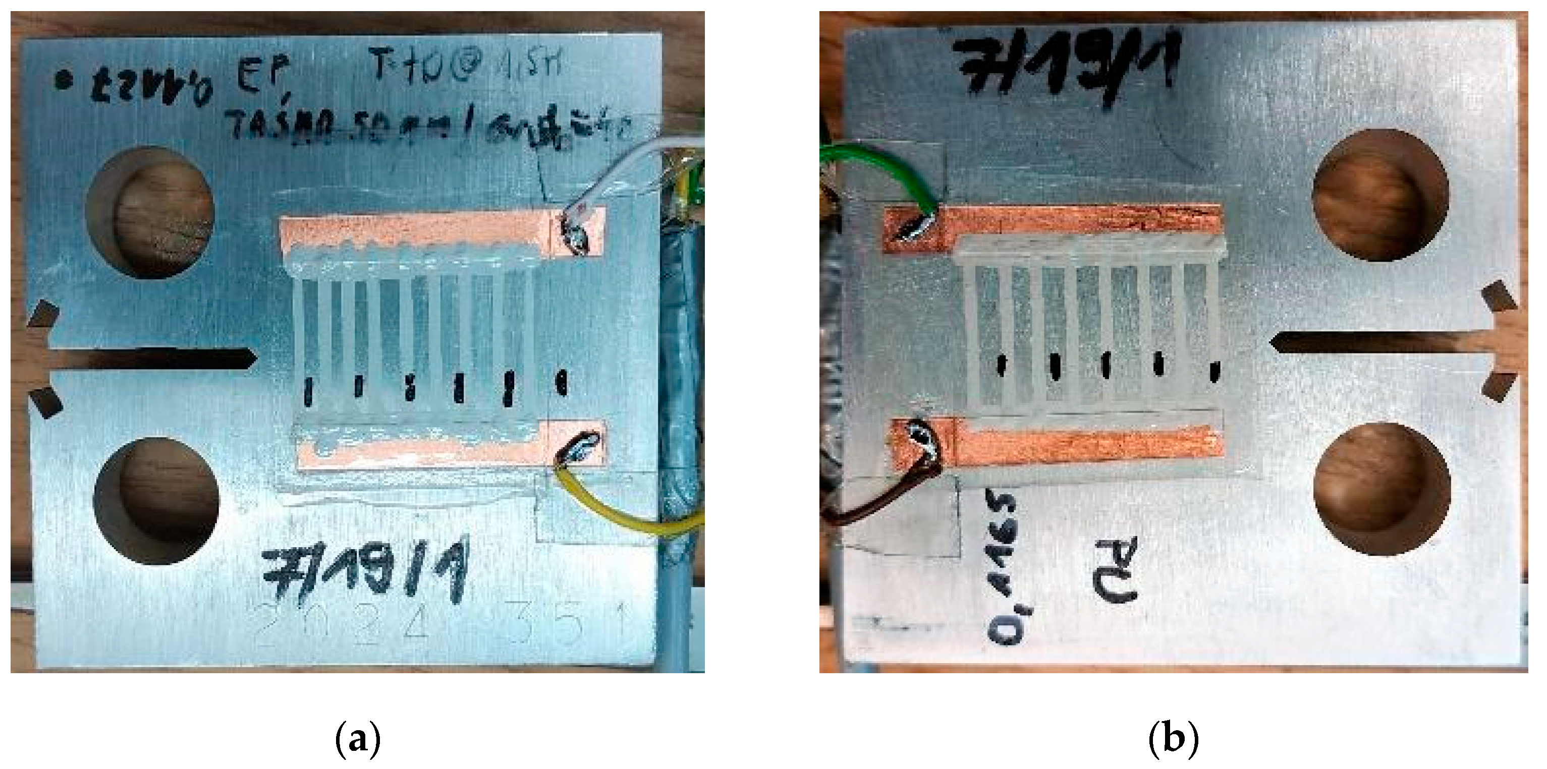
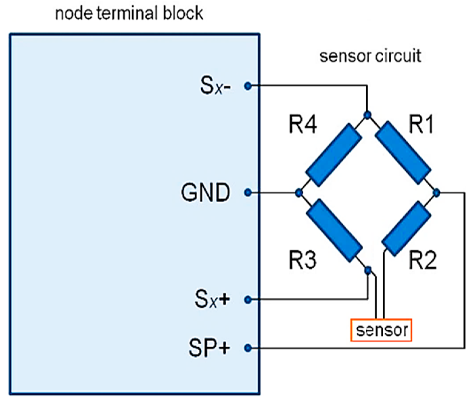
2.1. Crack Propagation Sensors as Silver Conductive Grid
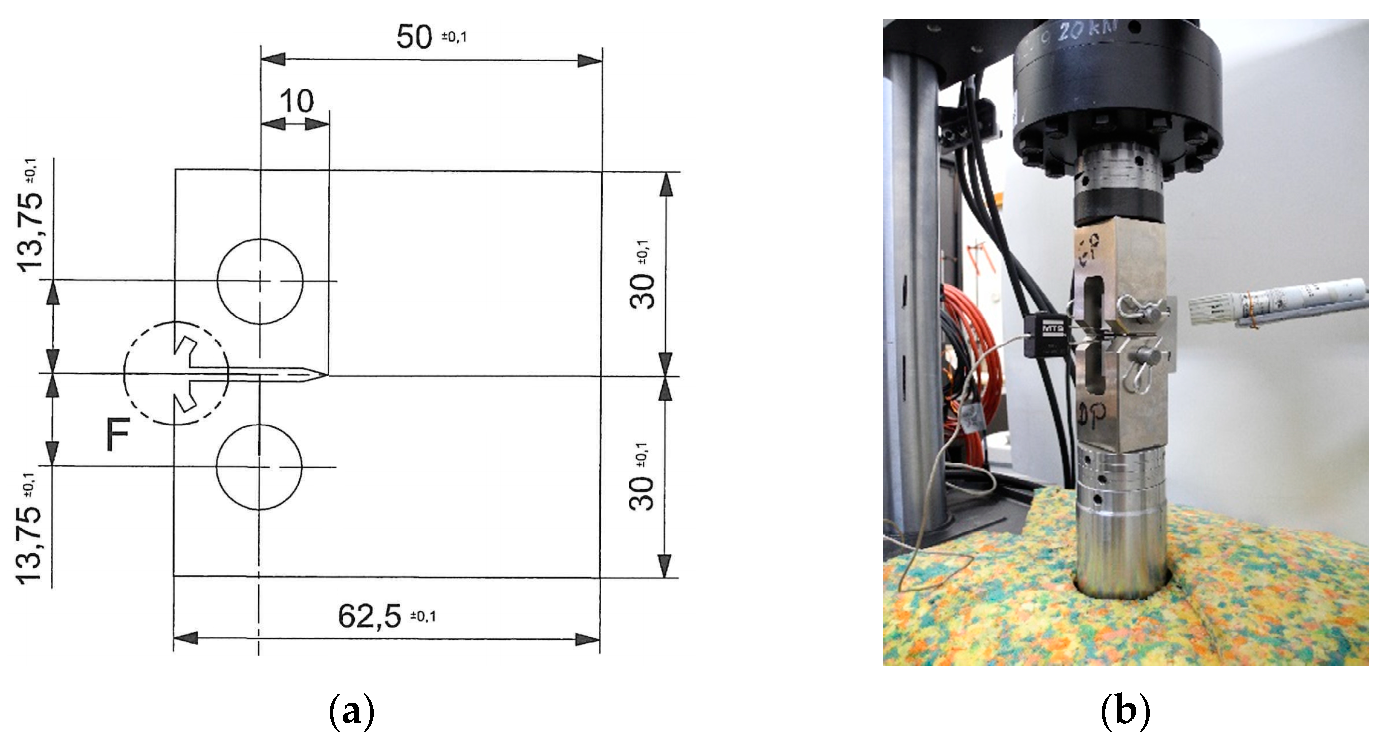
2.2. Test Procedure and Additional Instrumentation of Fatigue Machine
2.3. Crack Prediction with ARIMA Modeling
3. Results
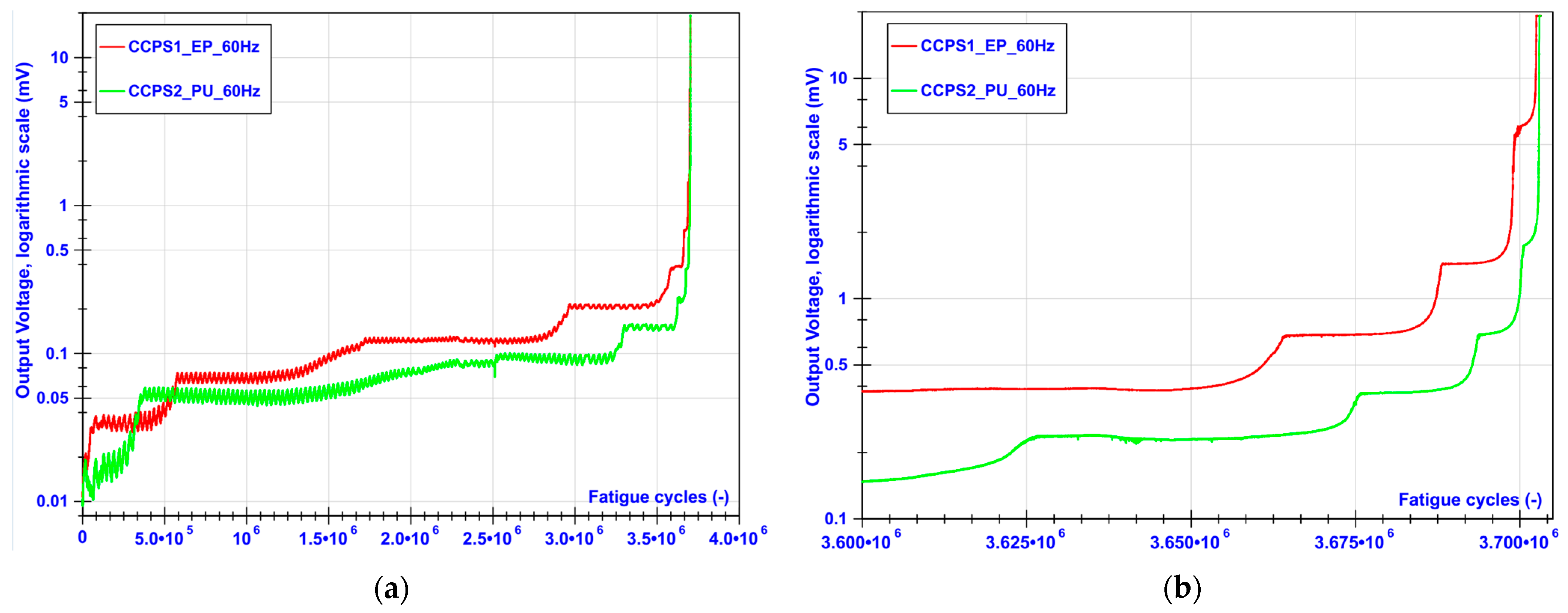
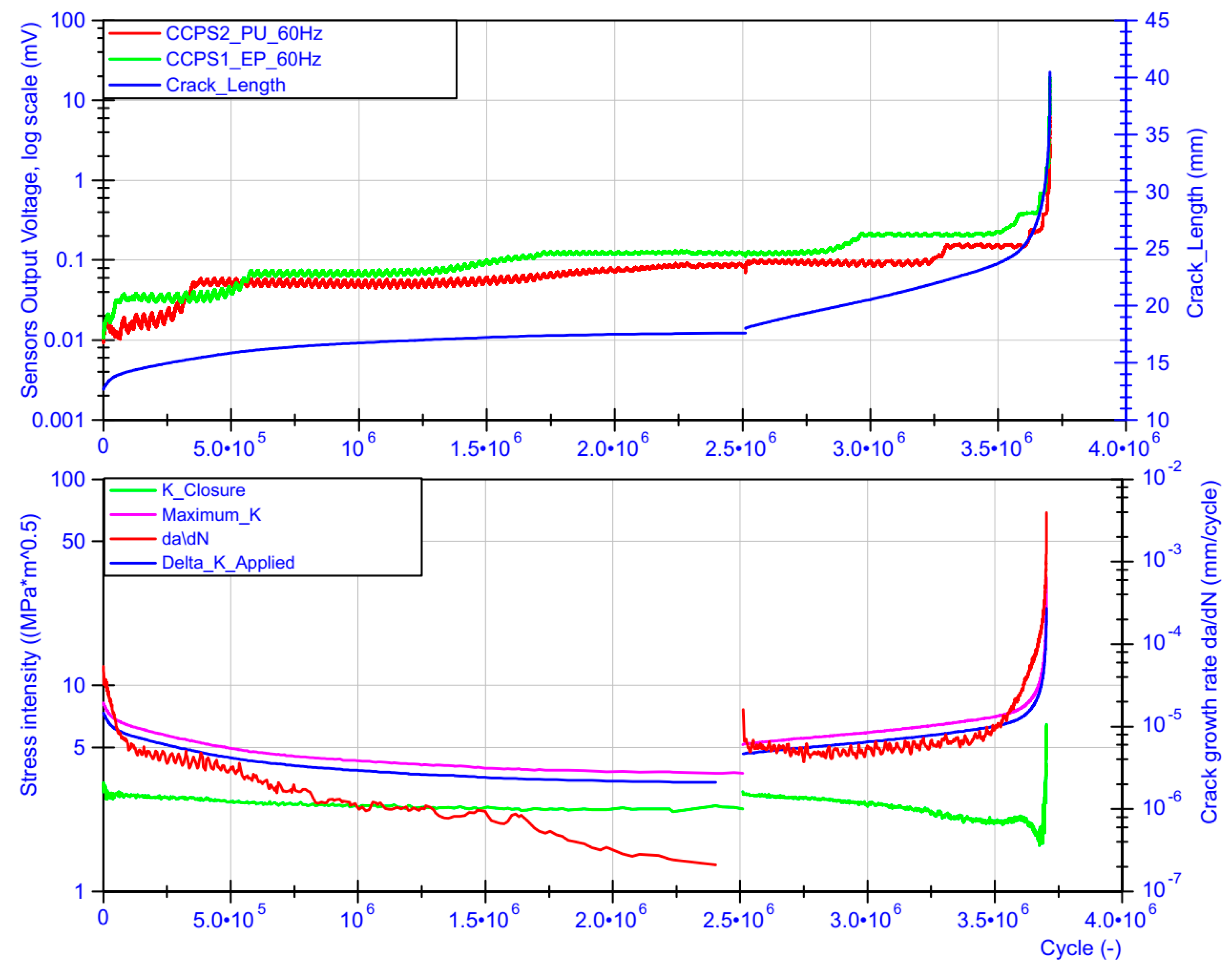
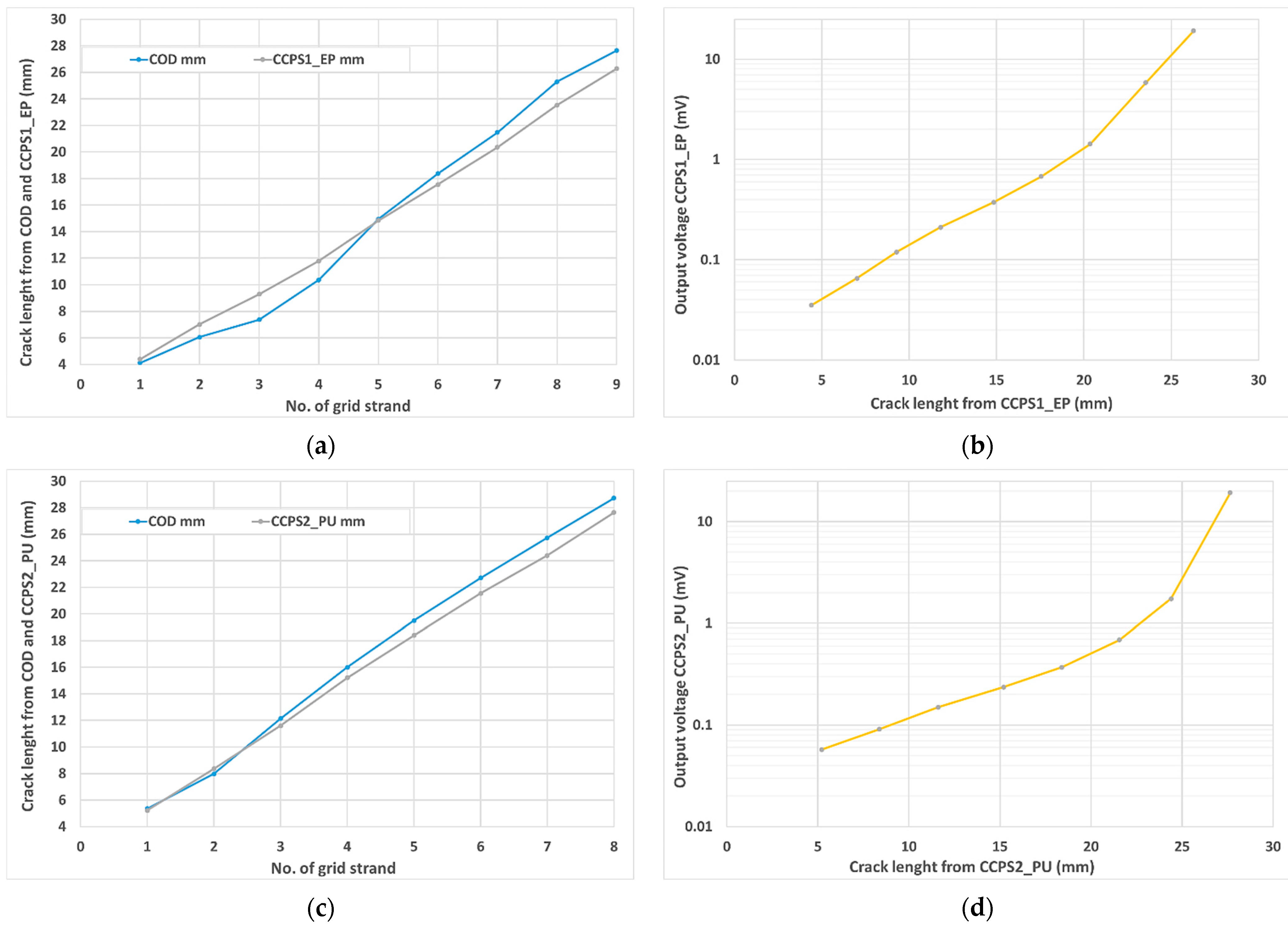
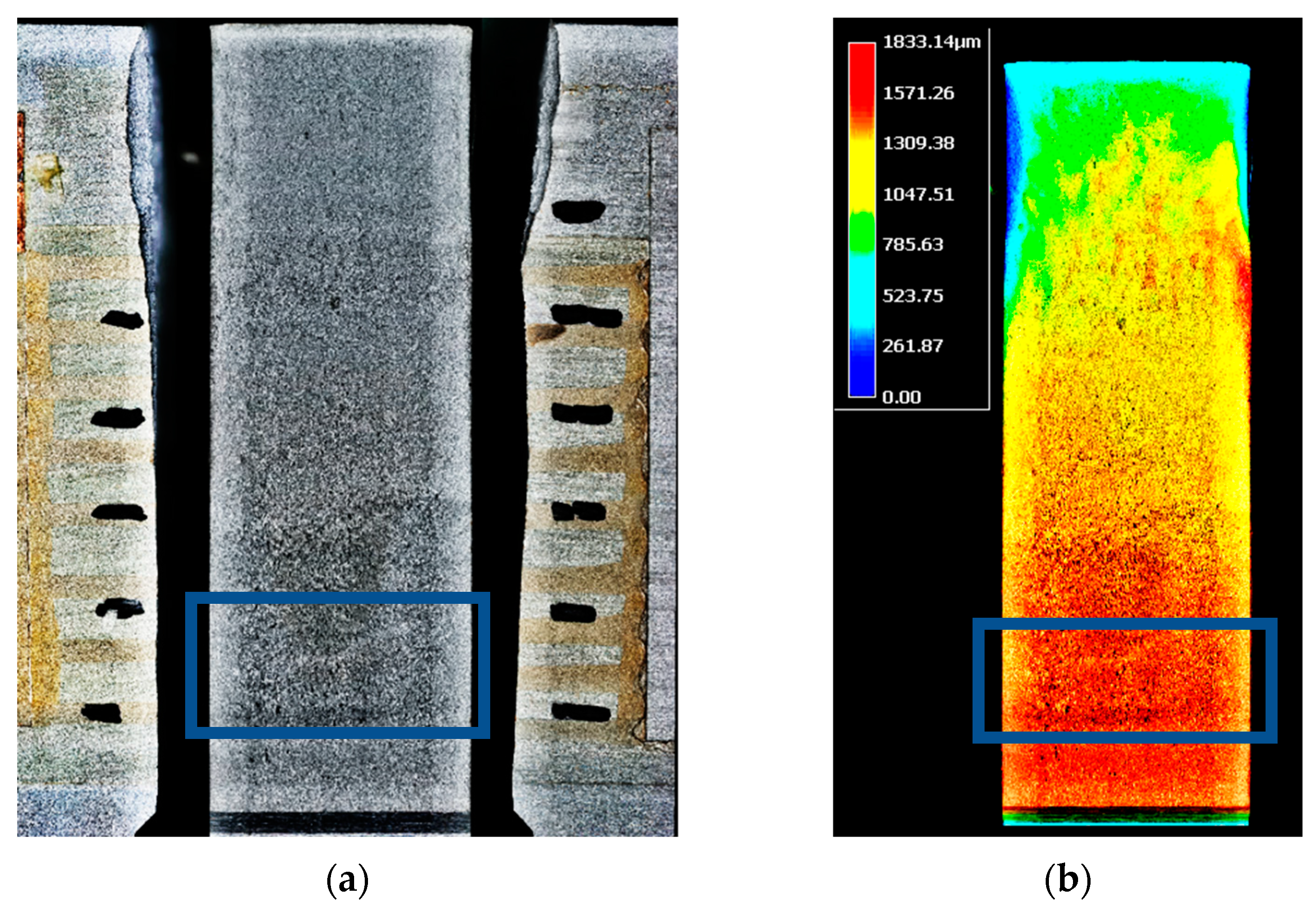
3.1. Continuous Crack Propagation Monitoring Test
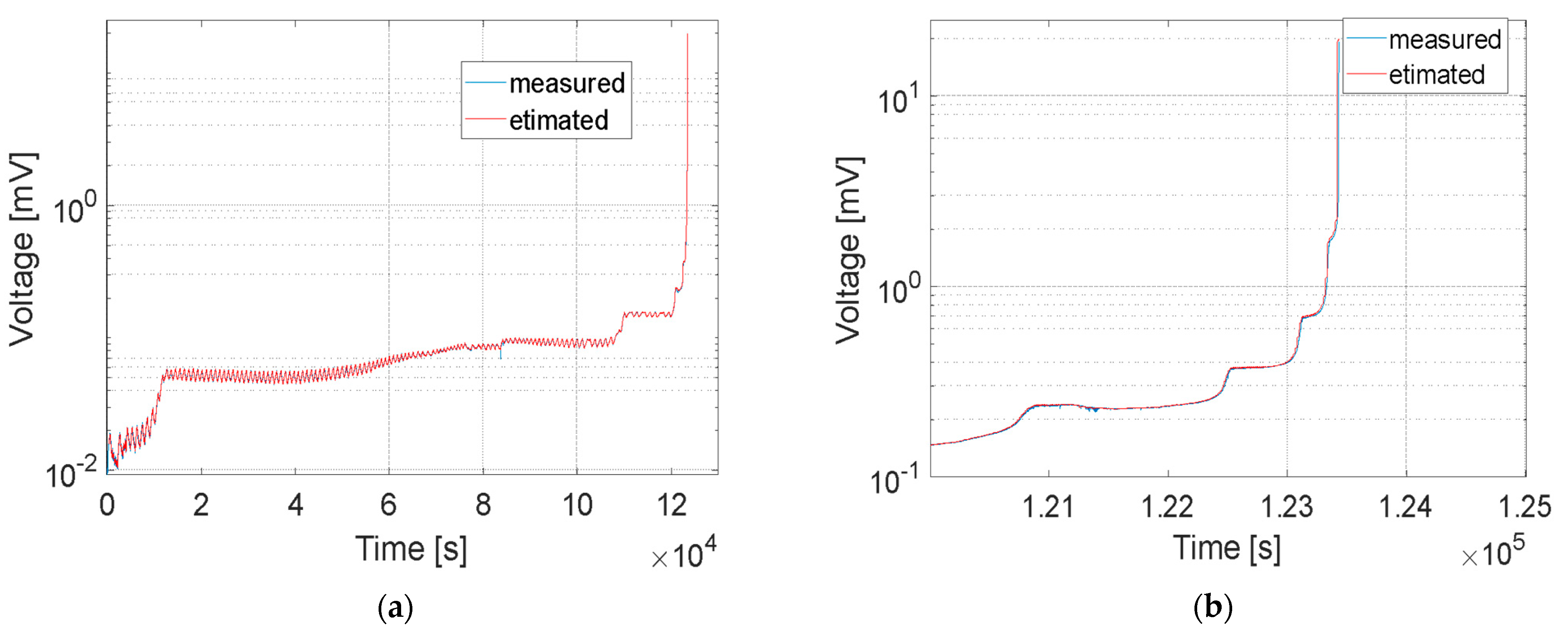
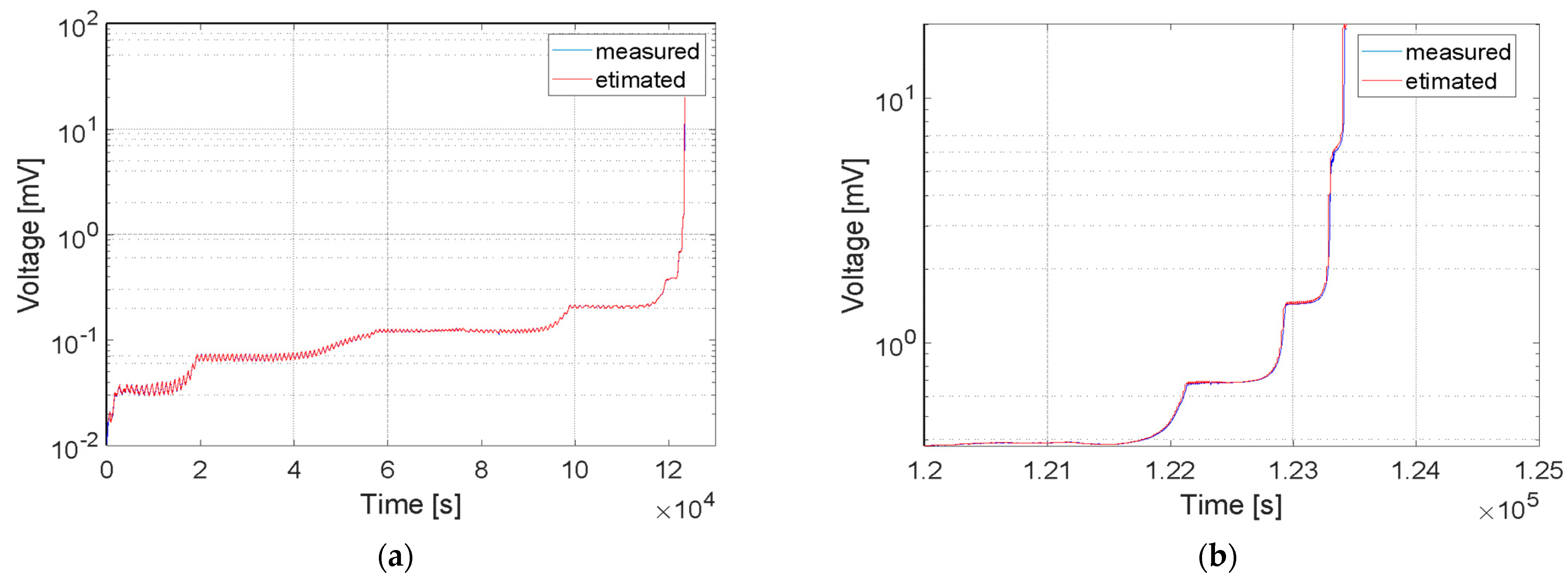
3.2. ARIMA Time Series Analysis
4. Discussion
Author Contributions
Funding
Institutional Review Board Statement
Informed Consent Statement
Data Availability Statement
Acknowledgments
Conflicts of Interest
References
- Kurnyta, A.; Kowalczyk, K.; Baran, M.; Dziendzikowski, M.; Dragan, K. The use of silver conductive paint for crack propagation sensor customization. In Proceedings of the 2021 IEEE 8th International Workshop on Metrology for AeroSpace (MetroAeroSpace), Naples, Italy, 23–25 June 2021; pp. 631–635. [Google Scholar] [CrossRef]
- SAE International. Guidelines for Implementation of Structural Health Monitoring on Fixed Wing Aircraft; ARP 6461; SAE International: Warrendale, PA, USA, 2013. [Google Scholar]
- Azzam, H. MASSAAG Paper 123: Development, Validation, Verification and Certification of Structural Health Monitoring Systems for Military Aircraft; The Military Aircraft Structural Airworthiness Advisory Group: Bristol, UK, 2015. [Google Scholar]
- Giurgiutiu, V. Tuned Lamb Wave Excitation and Detection with Piezoelectric Wafer Active Sensors for Structural Health Monitoring. J. Intell. Mater. Syst. Struct. 2005, 16, 291–305. [Google Scholar] [CrossRef]
- Stepinski, T.; Uhl, T.; Staszewski, W. Advanced Structural Damage Detection: From Theory to Engineering Applications; John Wiley & Sons: Chichester, UK, 2013. [Google Scholar]
- Memmolo, V.; Pasquino, N.; Ricci, F. Experimental characterization of a damage detection and localization system for composite structures. Measurement 2018, 129, 381–388. [Google Scholar] [CrossRef]
- Kahandawa, G.; Epaarachchi, J.; Wang, H.; Lau, K.T. Use of FBG sensors for SHM in aerospace structures. Photonic Sens. 2012, 2, 203–214. [Google Scholar] [CrossRef] [Green Version]
- Terroba, F.; Frövel, M.; Atienza, R. Structural health and usage monitoring of an unmanned turbojet target drone. Struct. Health Monit. 2018, 18, 635–650. [Google Scholar] [CrossRef]
- Molent, L.; Aktepe, B. Review of fatigue monitoring of agile military aircraft. Fatigue Fract. Eng. Mater. Struct. 2000, 23, 767–785. [Google Scholar] [CrossRef]
- Kurnyta, A.; Zieliński, W.; Reymer, P.; Dziendzikowski, M. Operational load monitoring system implementation for Su-22UM3K aging aircraft. In Structural Health Monitoring 2017; Chang, F., Kopsaftopoulo, F., Eds.; DEStech Publications, Inc.: Lancaster, PA, USA, 2017. [Google Scholar]
- Roach, D. Real time crack detection using mountable comparative vacuum monitoring sensors. Smart Struct. Syst. 2009, 5, 317–328. [Google Scholar] [CrossRef]
- Rulli, R.P.; Dotta, F.; da Silva, P.A. Flight Tests Performed by EMBRAER with SHM Systems. Key Eng. Mater. 2013, 558, 305–313. [Google Scholar] [CrossRef]
- Chen, T.; He, Y.; Du, J. A High-Sensitivity Flexible Eddy Current Array Sensor for Crack Monitoring of Welded Structures under Varying Environment. Sensors 2018, 18, 1780. [Google Scholar] [CrossRef] [Green Version]
- Jiao, S.; Cheng, L.; Li, X.; Li, P.; Ding, H. Monitoring fatigue cracks of a metal structure using an eddy current sensor. EURASIP J. Wirel. Commun. Netw. 2016, 188, 1–14. [Google Scholar] [CrossRef] [Green Version]
- Mabao, L.; Feng, H.; Hong, G.; Zhigang, L. The Crack-Detected Coating Sensor and Its Application in R&M of Aircrafts. In Proceedings of the 27th Congress of International Council of the Aeronautical Sciences, Nice, France, 19–24 January 2010. Paper ICAS2010-10.6ST. [Google Scholar]
- Hou, B.; He, Y.; Cui, R.; Gao, C.; Zhang, T. Crack monitoring method based on Cu coating sensor and electrical potential technique for metal structure. Chin. J. Aeronaut. 2015, 28, 932–938. [Google Scholar] [CrossRef] [Green Version]
- Deng, G.; Nasu, K.; Redda, T.R.; Nakanishi, T. Fatigue Crack Length Measurement Method with an Ion Sputtered Film. In Fracture of Nano and Engineering Materials and Structures; Gdoutos, E.E., Ed.; Springer: Dordrecht, The Netherlands, 2006; pp. 437–445. [Google Scholar] [CrossRef]
- Pour-Ghaz, M.; Weiss, W. Detecting the time and location of cracks using electrically conductive surfaces. Cem. Concr. Compos. 2011, 33, 116–123. [Google Scholar] [CrossRef]
- Ahmed, S.; Schumacher, T.; Thostenson, E.T.; McConnell, J. Performance Evaluation of a Carbon Nanotube Sensor for Fatigue Crack Monitoring of Metal Structures. Sensors 2020, 20, 4383. [Google Scholar] [CrossRef] [PubMed]
- Kharroub, S.; Laflamme, S.; Song, C.; Qiao, D.; Phares, B.; Li, J. Smart sensing skin for detection and localization of fatigue cracks. Smart Mater. Struct. 2015, 24, 065004. [Google Scholar] [CrossRef] [Green Version]
- Gallo, G.J.; Thostenson, E.T. Electrical characterization and modeling of carbon nanotube and carbon fiber self-sensing composites for enhanced sensing of microcracks. Mater. Today Commun. 2015, 3, 17–26. [Google Scholar] [CrossRef]
- Thomas, A.J.; Kim, J.J.; Tallman, T.N.; Bakis, C.E. Damage detection in self-sensing composite tubes via electrical impedance tomography. Compos. Part B Eng. 2019, 177, 107276. [Google Scholar] [CrossRef]
- Viets, C.; Kaysser, S.; Schulte, K. Damage mapping of GFRP via electrical resistance measurements using nanocomposite epoxy matrix systems. Compos. Part B: Eng. 2014, 65, 80–88. [Google Scholar] [CrossRef]
- Park, J.-M.; Kim, D.-S.; Kim, S.-J.; Kim, P.-G.; Yoon, D.-J.; DeVries, K.L. Inherent sensing and interfacial evaluation of carbon nanofiber and nanotube/epoxy composites using electrical resistance measurement and micromechanical technique. Compos. Part B Eng. 2007, 38, 847–861. [Google Scholar] [CrossRef]
- Kurnyta, A. Application of resistive ladder sensor for detection and quantification of fatigue cracks in aircraft structure. Mon. Sci. Tech. J. PAR–Pomiary Autom. Robot. 2013, 2, 558–563. (In Polish) [Google Scholar]
- Kurnyta, A.; Dziendzikowski, M.; Dragan, K.; Leski, A. Approach to Health Monitoring of an Aircraft Structure with Resistive Ladder Sensors During Full Scale Fatigue Test. In Proceedings of the EWSHM—7th European Workshop on Structural Health Monitoring, Nantes, France, 8–11 July 2014. [Google Scholar]
- Banaezadeh, F. ARIMA-modeling based prediction mechanism in object tracking sensor networks. In Proceedings of the 2015 7th Conference on Information and Knowledge Technology (IKT), Urmia, Iran, 26–28 May 2015; pp. 1–5. [Google Scholar] [CrossRef]
- Agrawal, R.K.; Adhikari, R. An Introductory Study on Time Series Modeling and Forecasting. arXiv 2013, arXiv:1302.6613. [Google Scholar]
- Box GE, P.; Jenkins, G.M.; Reinsel, G.C. Time Series Analysis: Forecasting and Control, 3rd ed.; Prentice Hall: Englewood Cliffs, NJ, USA, 1994. [Google Scholar]
- Matlab Help Documentation. Available online: https://www.mathworks.com/help/matlab/ (accessed on 20 September 2021).


Publisher’s Note: MDPI stays neutral with regard to jurisdictional claims in published maps and institutional affiliations. |
© 2021 by the authors. Licensee MDPI, Basel, Switzerland. This article is an open access article distributed under the terms and conditions of the Creative Commons Attribution (CC BY) license (https://creativecommons.org/licenses/by/4.0/).
Share and Cite
Kurnyta, A.; Baran, M.; Kurnyta-Mazurek, P.; Kowalczyk, K.; Dziendzikowski, M.; Dragan, K. The Experimental Verification of Direct-Write Silver Conductive Grid and ARIMA Time Series Analysis for Crack Propagation. Sensors 2021, 21, 6916. https://doi.org/10.3390/s21206916
Kurnyta A, Baran M, Kurnyta-Mazurek P, Kowalczyk K, Dziendzikowski M, Dragan K. The Experimental Verification of Direct-Write Silver Conductive Grid and ARIMA Time Series Analysis for Crack Propagation. Sensors. 2021; 21(20):6916. https://doi.org/10.3390/s21206916
Chicago/Turabian StyleKurnyta, Artur, Marta Baran, Paulina Kurnyta-Mazurek, Kamil Kowalczyk, Michał Dziendzikowski, and Krzysztof Dragan. 2021. "The Experimental Verification of Direct-Write Silver Conductive Grid and ARIMA Time Series Analysis for Crack Propagation" Sensors 21, no. 20: 6916. https://doi.org/10.3390/s21206916