
Clutter Suppression for Indoor Self-Localization Systems by Iteratively Reweighted Low-Rank Plus Sparse Recovery

 , , , , , and
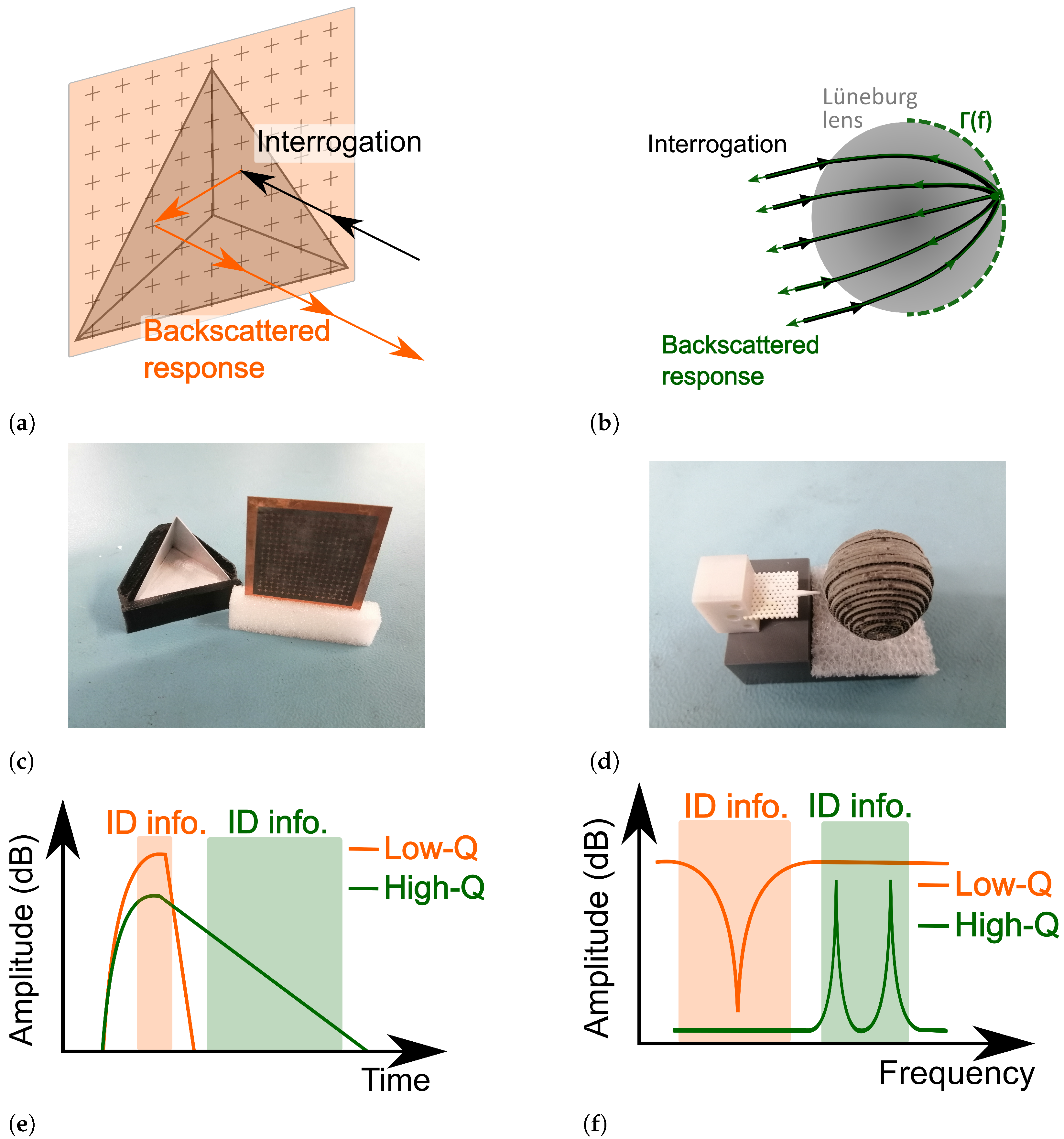
Abstract
:1. Introduction
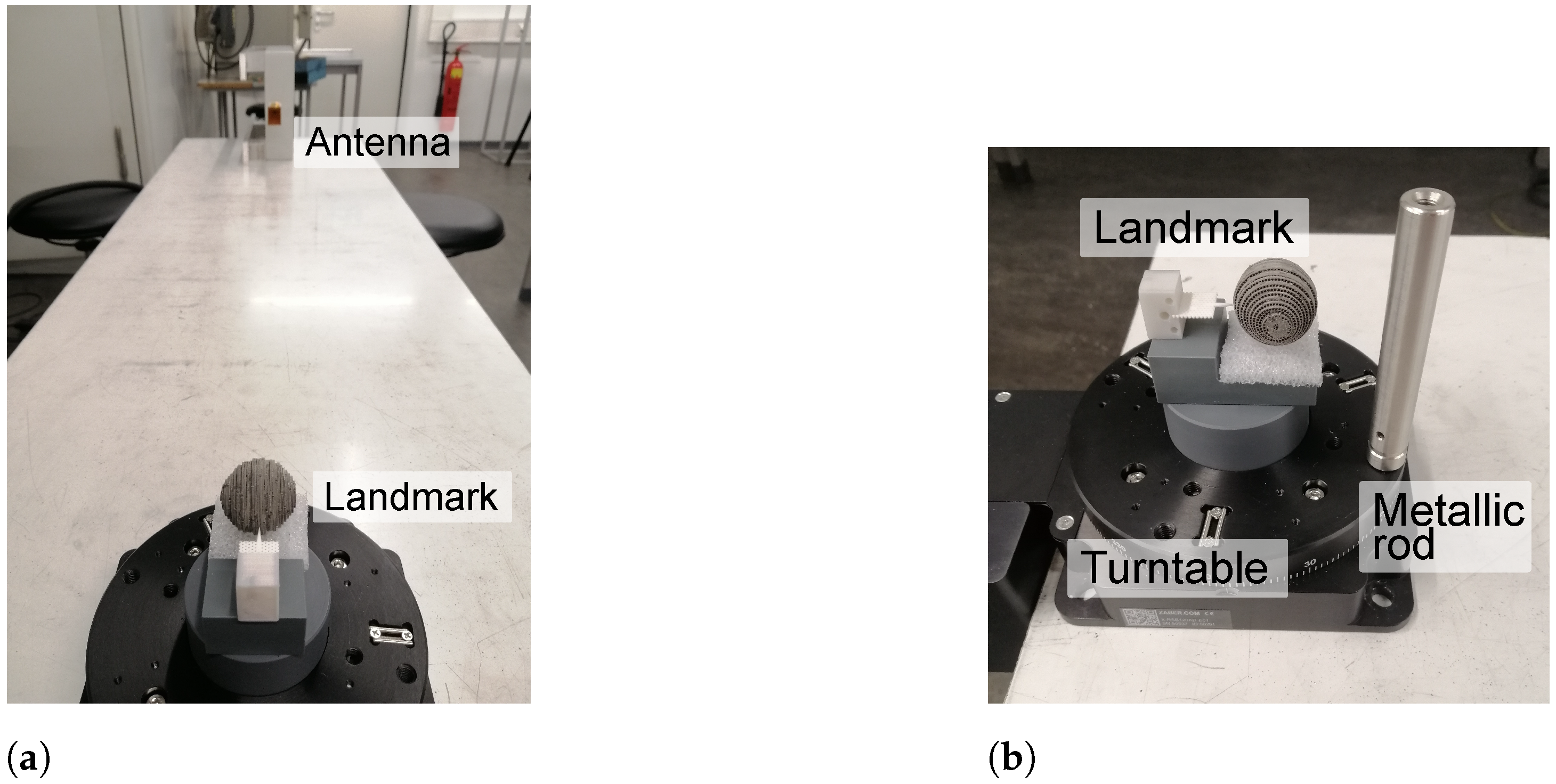
2. Localization Tag Landmarks
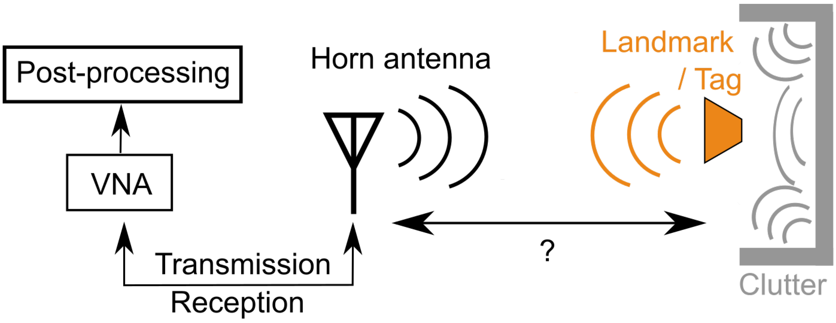
3. System Model
4. Clutter Suppression for High-Q and Low-Q Tags
4.1. Low-Rank Plus Sparse Recovery (RPCA) for Clutter Suppression
4.2. Low-Rank Plus Sparse Recovery (RPCA) for Low-Q Tag
4.3. Parameter Selection for ADMM Based Iterative RPCA Algorithm
5. Measurement Results and Discussion
5.1. Low-Q Landmark
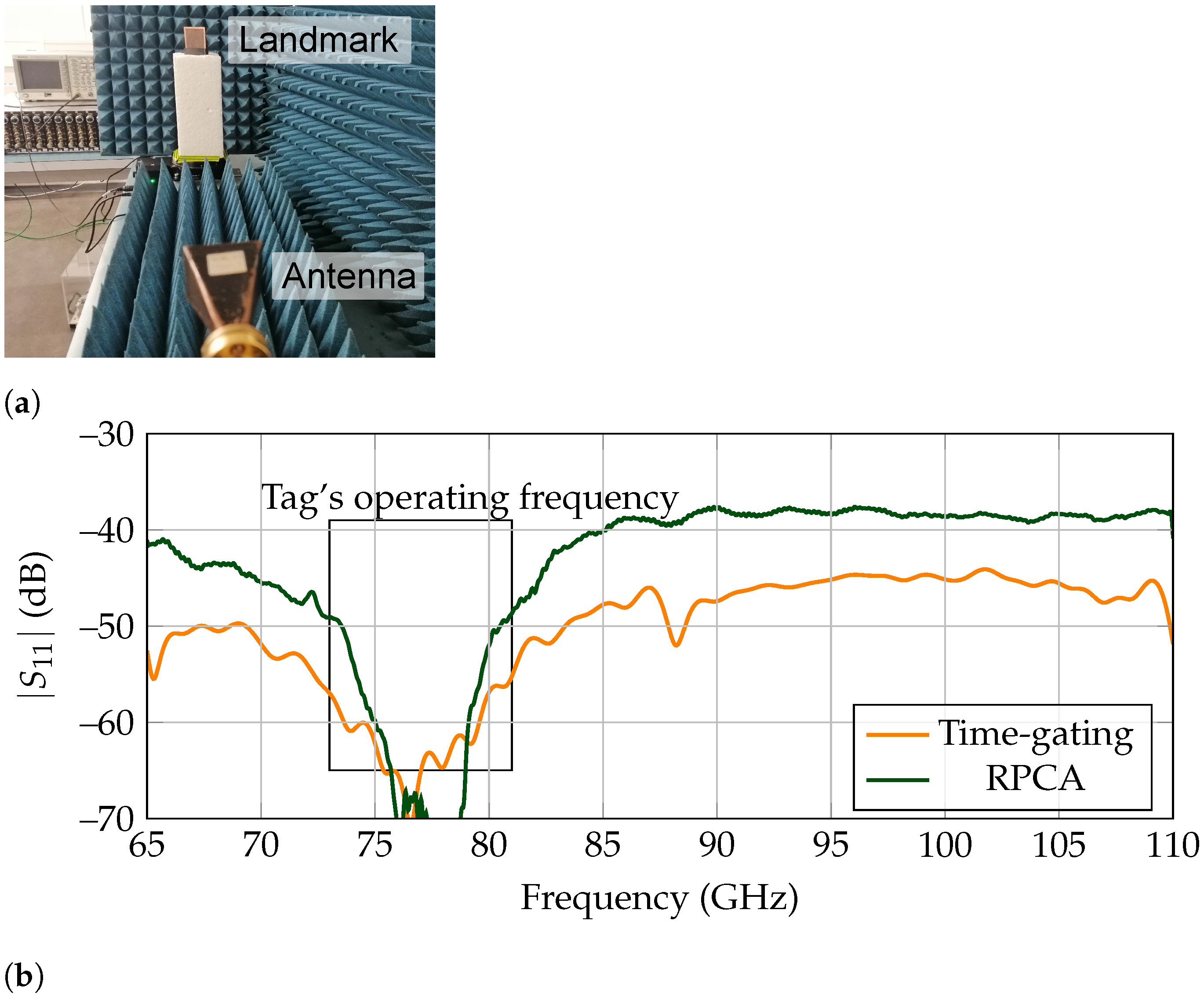
5.1.1. Characterization
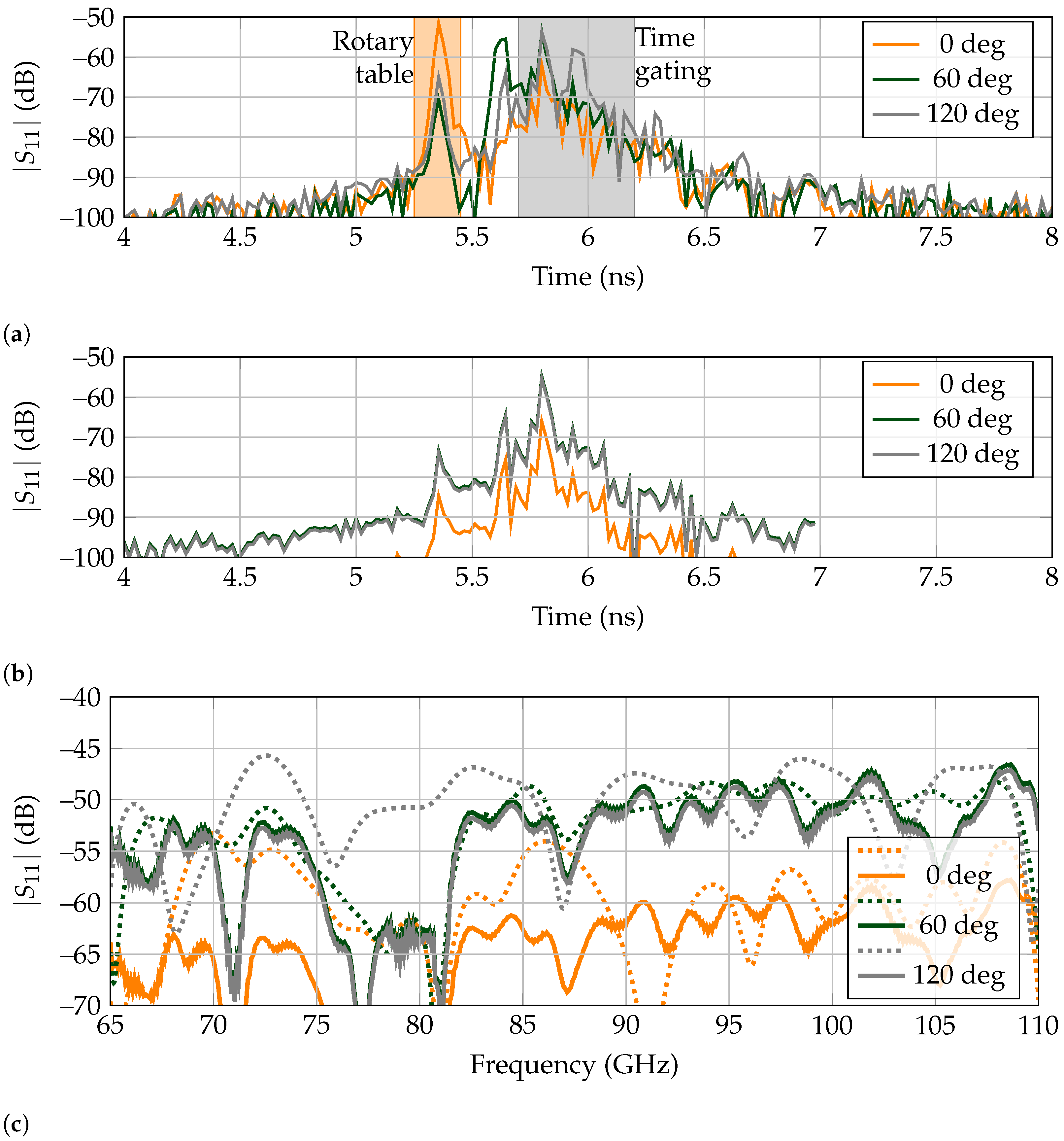
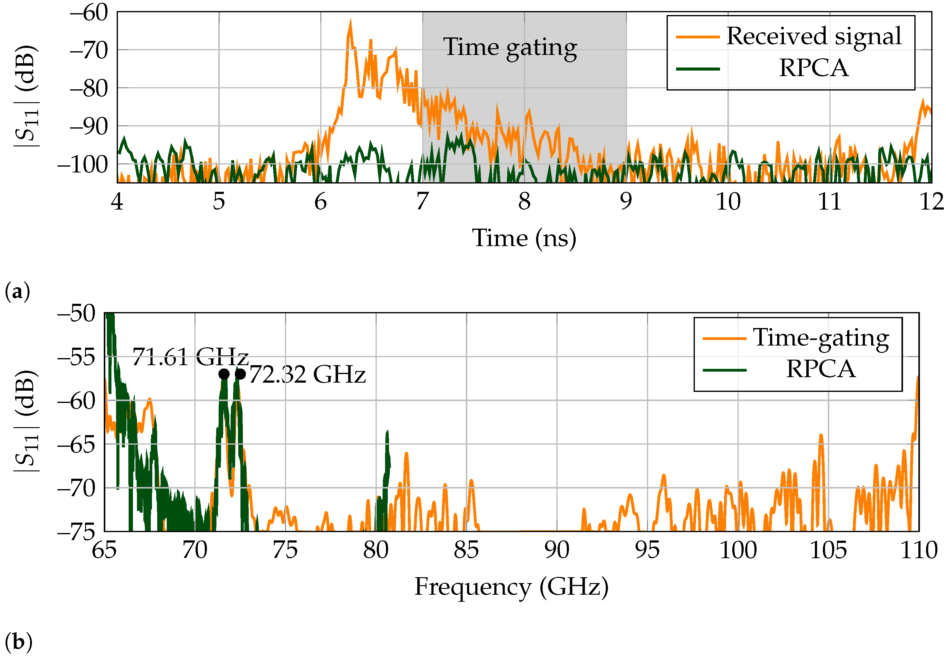
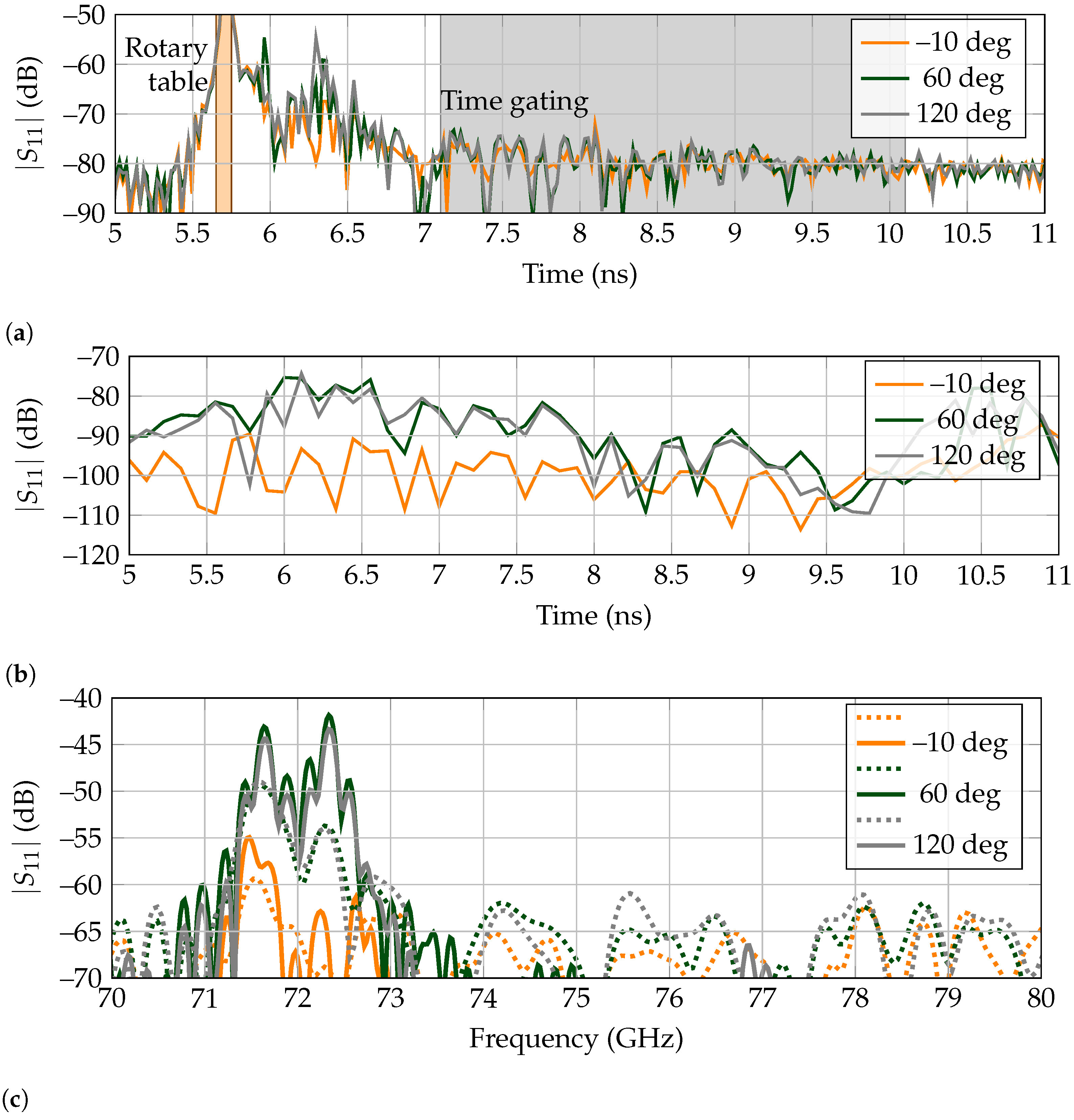
5.1.2. Cluttered Measurements
- The early reflections of the antenna, resulting of a mismatch between the horn antenna and the WR10 extension.
- Reflections on the “ground” i.e., the table that supports the set-up.
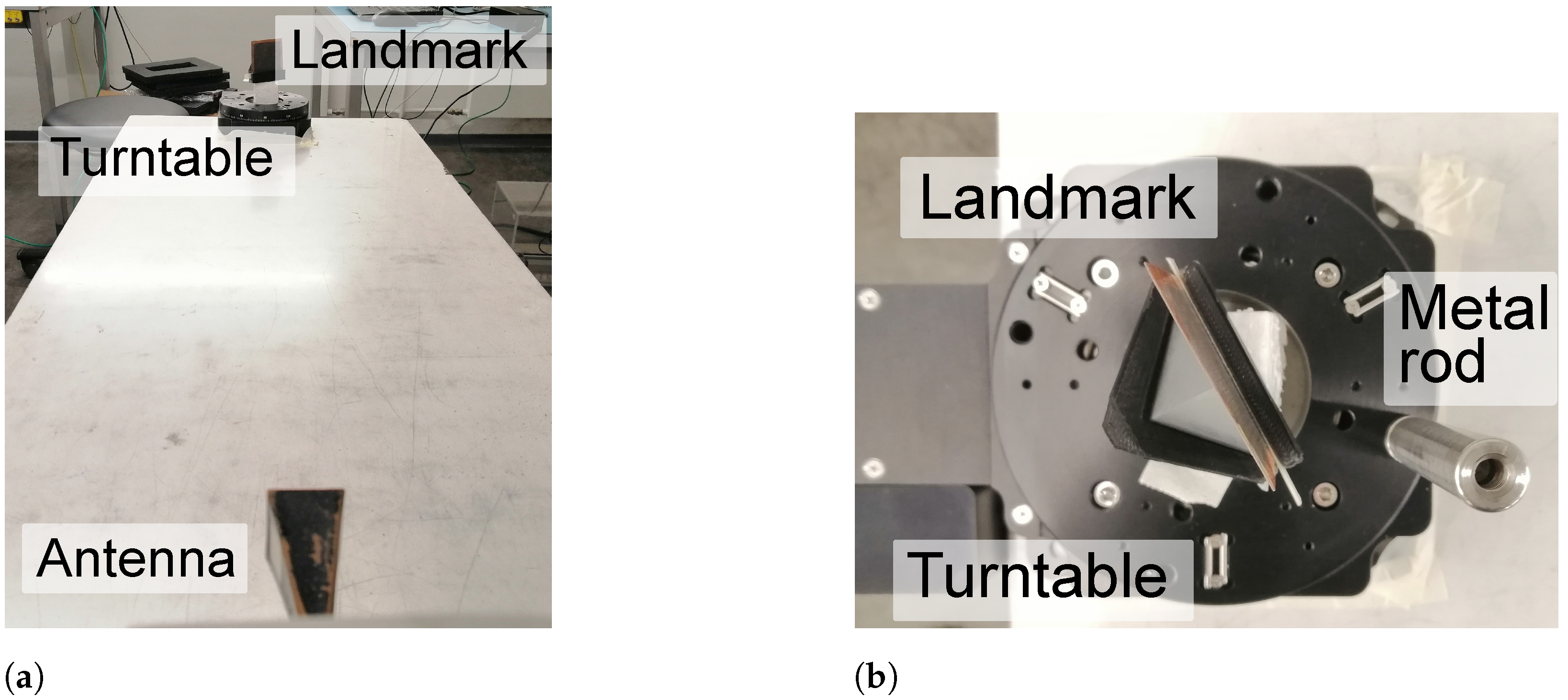
- Reflection on the measurement turn-table, which is completely made up of metal.
- Late environmental clutter owing to the surrounding laboratory room, such as reflection on columns, equipment, or walls.
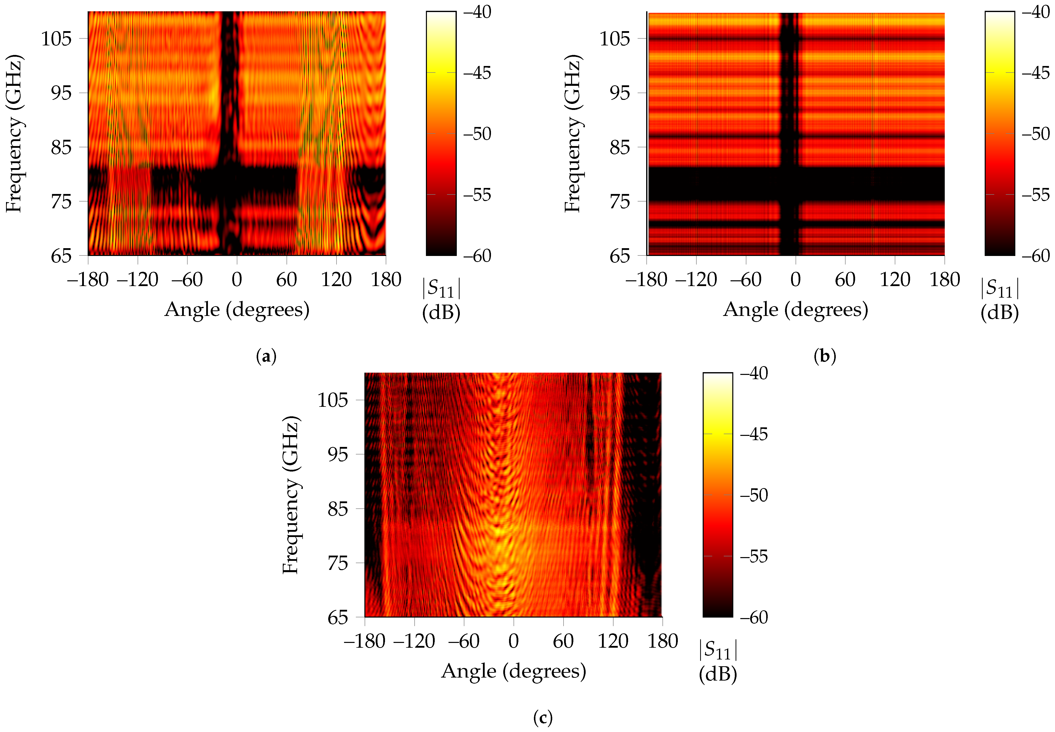
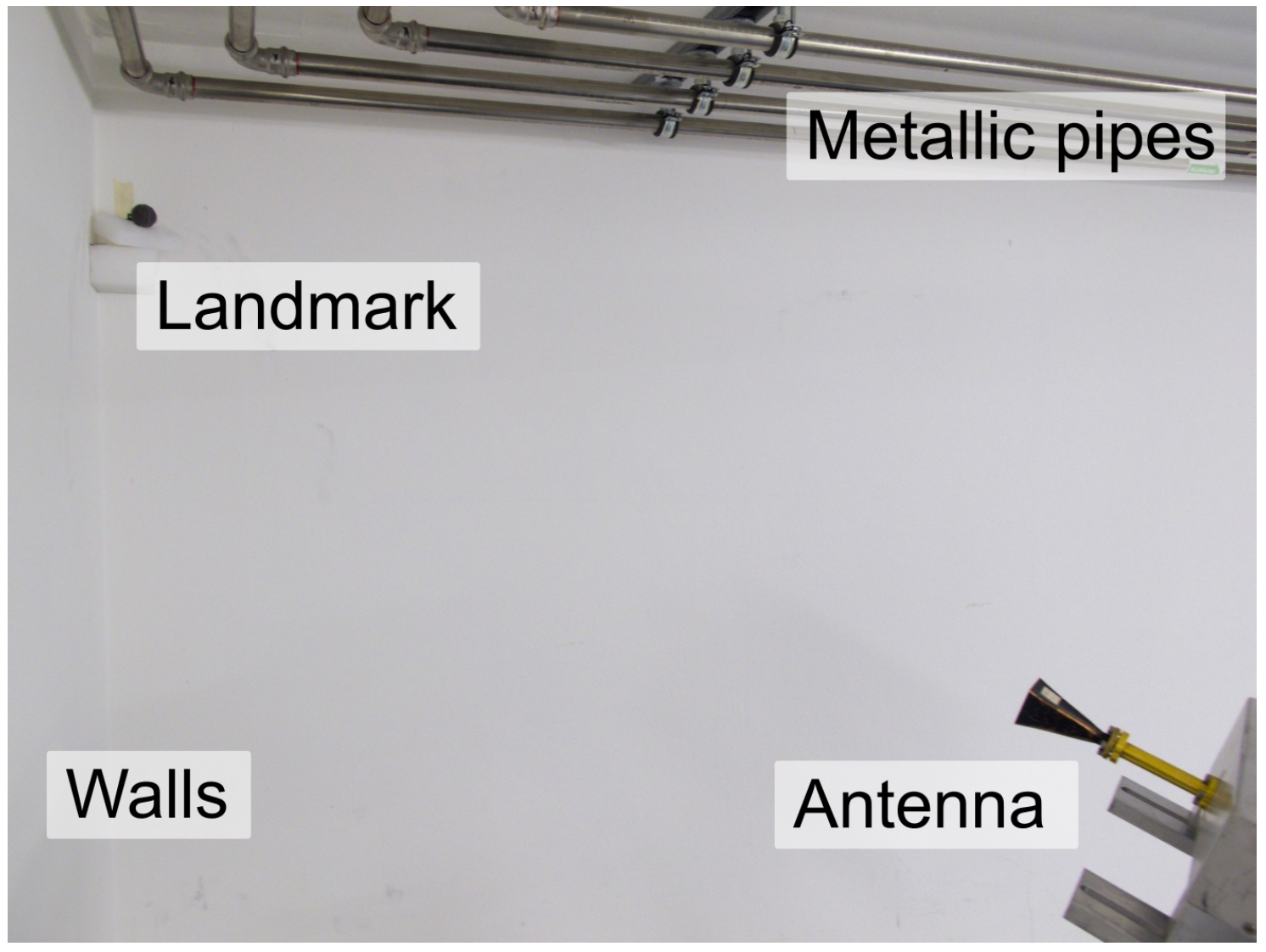
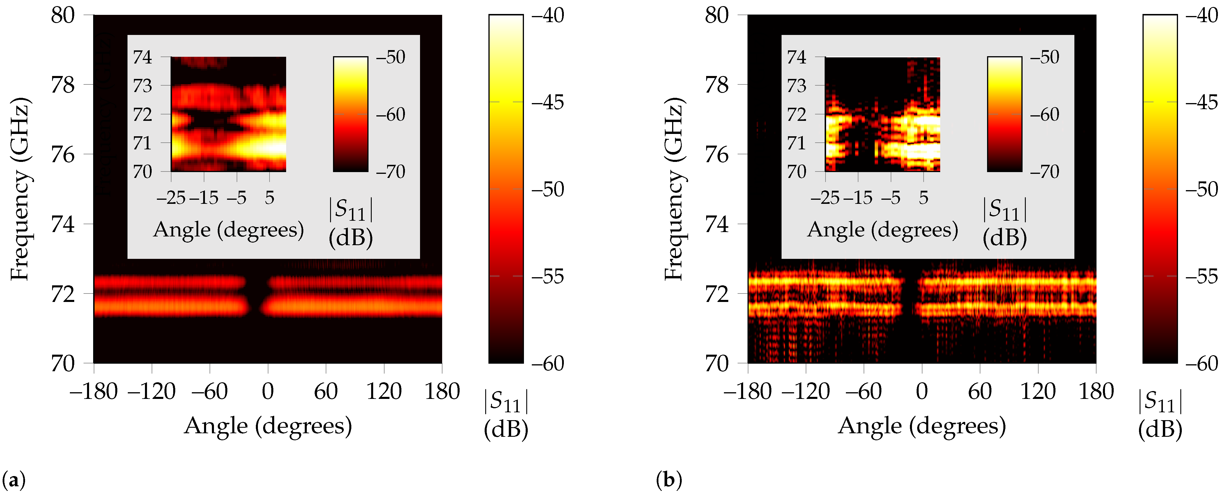
5.1.3. Indoor Scenario
5.2. High-Q Landmark
5.2.1. Characterization
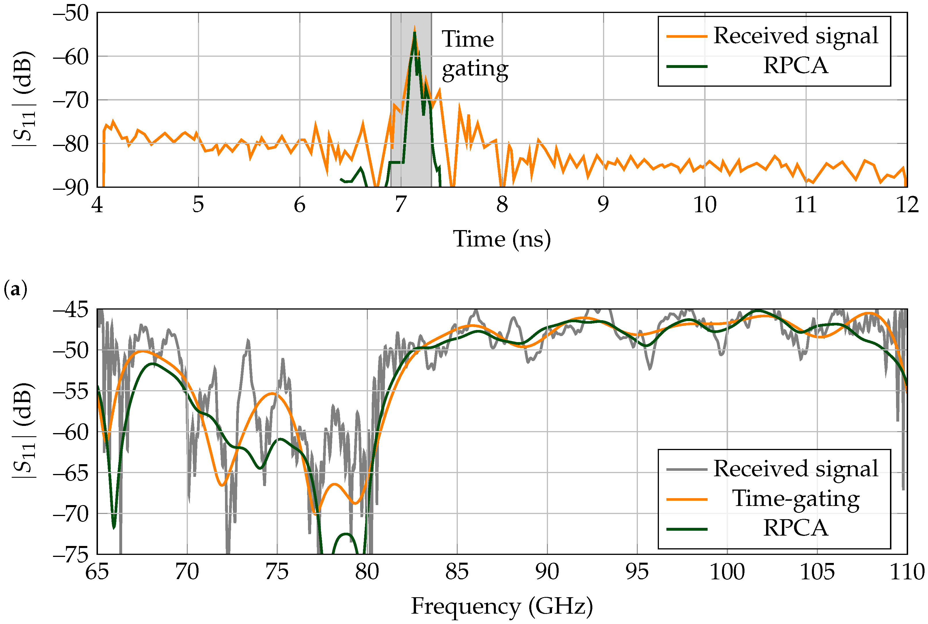
5.2.2. Cluttered Measurements
5.2.3. Indoor Scenario
6. Conclusions
Author Contributions
Funding
Institutional Review Board Statement
Informed Consent Statement
Data Availability Statement
Conflicts of Interest
References
- Sanpechuda, T.; Kovavisaruch, L. A review of RFID Localization: Application and Techniques. In Proceedings of the 2008 5th International Conference on Electrical Engineering/Electronics, Computer, Telecommunications and Information Technology, Krabi, Thailand, 14–17 May 2008; IEEE: Piscataway, NJ, USA, 2008; pp. 769–772. [Google Scholar]
- Chabbar, H.; Chami, M. Indoor localization using Wi-Fi method based on Fingerprinting Technique. In Proceedings of the 2017 International Conference on Wireless Technologies, Embedded and Intelligent Systems (WITS), Fez, Morocco, 19–20 April 2017; pp. 1–5. [Google Scholar] [CrossRef]
- Basri, C.; El Khadimi, A. Survey on indoor localization system and recent advances of WIFI fingerprinting technique. In Proceedings of the 2016 5th International Conference on Multimedia Computing and Systems (ICMCS), Marrakech, Morocco, 2016, 29 September–1 October; pp. 253–259. [CrossRef]
- Jin, G.Y.; Lu, X.Y.; Park, M.S. An indoor localization mechanism using active RFID tag. In Proceedings of the IEEE International Conference on Sensor Networks, Ubiquitous, and Trustworthy Computing (SUTC’06), Taichung, Taiwan, 5–7 June 2006; Volume 1, p. 4. [Google Scholar] [CrossRef]
- French, P.; Krijnen, G.; Roozeboom, F. Precision in harsh environments. Microsyst. Nanoeng. 2016, 2, 16048. [Google Scholar] [CrossRef]
- Abbas, A.A.; El-Absi, M.; Abuelhaijay, A.; Solbach, K.; Kaiser, T. THz Passive RFID Tag Based on Dielectric Resonator Linear Array. In Proceedings of the 2019 Second International Workshop on Mobile Terahertz Systems (IWMTS), Bad Neuenahr, Germany, 1–3 July 2019; pp. 1–5. [Google Scholar] [CrossRef]
- Jiménez-Sáez, A.; Alhaj-Abbas, A.; Schüßler, M.; Abuelhaija, A.; El-Absi, M.; Sakaki, M.; Samfaß, L.; Benson, N.; Hoffmann, M.; Jakoby, R.; et al. Frequency-coded mm-wave tags for self-localization system using dielectric resonators. J. Infrared Millim. Terahertz Waves 2020, 41, 908–925. [Google Scholar] [CrossRef]
- Soltanaghaei, E.; Dongare, A.; Prabhakara, A.; Kumar, S.; Rowe, A.; Whitehouse, K. TagFi: Locating Ultra-Low Power WiFi Tags Using Unmodified WiFi Infrastructure. In Proceedings of the ACM on Interactive, Mobile, Wearable and Ubiquitous Technologies, Cancun, Mexico, 21–26 September 2021; Volume 5, pp. 1–29. [Google Scholar]
- Kadera, P.; Jiménez-Sáez, A.; Schmitt, L.; Schüßler, M.; Hoffmann, M.; Lacik, J.; Jakoby, R. Frequency Coded Retroreflective Landmark for 230 GHz Indoor Self-Localization Systems. In Proceedings of the 2021 15th European Conference on Antennas and Propagation (EuCAP), Dusseldorf, Germany, 22–26 March 2021; pp. 1–5. [Google Scholar] [CrossRef]
- El-Absi, M.; Abbas, A.A.h.; Abuelhaija, A.; Solbach, K.; Kaiser, T. Chipless RFID Infrastructure Based Self-Localization: Testbed Evaluation. IEEE Trans. Veh. Technol. 2020, 69, 7751–7761. [Google Scholar] [CrossRef]
- Kyösti, P.; Tervo, N.; Berg, M.; Leinonen, M.E.; Nevala, K.; Pärssinen, A. Measured Blockage Effect of a Finger and Similar Small Objects at 300 GHz. In Proceedings of the 2021 15th European Conference on Antennas and Propagation (EuCAP), Dusseldorf, Germany, 22–26 March 2021; pp. 1–5. [Google Scholar] [CrossRef]
- Khan, U.S.; Al-Nuaimy, W. Background removal from GPR data using eigenvalues. In Proceedings of the XIII Internarional Conference on Ground Penetrating Radar, Lecce, Italy, 21–25 June 2010; pp. 1–5. [Google Scholar]
- Yoon, Y.S.; Amin, M.G. Spatial filtering for wall-clutter mitigation in through-the-wall radar imaging. IEEE Trans. Geosci. Remote Sens. 2009, 47, 3192–3208. [Google Scholar] [CrossRef]
- Wang, J.; Ding, M.; Yarovoy, A. Interference Mitigation for FMCW Radar With Sparse and Low-Rank Hankel Matrix Decomposition. arXiv 2021, arXiv:2106.06748. [Google Scholar]
- Candès, E.J.; Li, X.; Ma, Y.; Wright, J. Robust principal component analysis? J. ACM 2011, 58, 1–37. [Google Scholar] [CrossRef]
- Yuan, X.; Yang, J. Sparse and low-rank matrix decomposition via alternating direction methods. Preprint 2009, 12. [Google Scholar]
- Tropp, J.A. Just relax: Convex programming methods for identifying sparse signals in noise. IEEE Trans. Inf. Theory 2006, 52, 1030–1051. [Google Scholar] [CrossRef] [Green Version]
- Bruckstein, A.M.; Donoho, D.L.; Elad, M. From sparse solutions of systems of equations to sparse modeling of signals and images. SIAM Rev. 2009, 51, 34–81. [Google Scholar] [CrossRef] [Green Version]
- Candes, E.J.; Romberg, J.K.; Tao, T. Stable signal recovery from incomplete and inaccurate measurements. Commun. Pure Appl. Math. A J. Issued Courant Inst. Math. Sci. 2006, 59, 1207–1223. [Google Scholar] [CrossRef] [Green Version]
- Candès, E.J.; Recht, B. Exact matrix completion via convex optimization. Found. Comput. Math. 2009, 9, 717–772. [Google Scholar] [CrossRef] [Green Version]
- Cai, J.; Candès, E.J.; Shen, Z. A singular value thresholding algorithm for matrix completion. SIAM J. Optim. 2010, 20, 1956–1982. [Google Scholar] [CrossRef]
- Fazel, M.; Hindi, H.; Boyd, S.P. A rank minimization heuristic with application to minimum order system approximation. In Proceedings of the 2001 American Control Conference. (Cat. No.01CH37148), Arlington, VA, USA, 25–27 June 2001; Volume 6, pp. 4734–4739. [Google Scholar]
- Candes, E.J.; Tao, T. The Power of Convex Relaxation: Near-Optimal Matrix Completion. IEEE Trans. Inf. Theory 2010, 56, 2053–2080. [Google Scholar] [CrossRef] [Green Version]
- Candès, E.J.; Wakin, M.B.; Boyd, S.P. Enhancing sparsity by reweighted ℓ1 minimization. J. Fourier Anal. Appl. 2008, 14, 877–905. [Google Scholar] [CrossRef]
- Daubechies, I.; DeVore, R.; Fornasier, M.; Güntürk, C.S. Iteratively reweighted least squares minimization for sparse recovery. Commun. Pure Appl. Math. A J. Issued Courant Inst. Math. Sci. 2010, 63, 1–38. [Google Scholar] [CrossRef] [Green Version]
- Mohan, K.; Fazel, M. Reweighted Nuclear norm minimization with application to system identification. In Proceedings of the 2010 American Control Conference, Baltimore, MD, USA, 30 June–2 July 2010; IEEE: Piscataway, NJ, USA, 2010; pp. 2953–2959. [Google Scholar]
- Gu, S.; Xie, Q.; Meng, D.; Zuo, W.; Feng, X.; Zhang, L. Weighted Nuclear norm minimization and its applications to low level vision. Int. J. Comput. Vis. 2017, 121, 183–208. [Google Scholar] [CrossRef]
- Lu, C.; Feng, J.; Yan, S.; Lin, Z. A Unified Alternating Direction Method of Multipliers by Majorization Minimization. IEEE Trans. Pattern Anal. Mach. Intell. 2018, 40, 527–541. [Google Scholar] [CrossRef] [Green Version]
- Jiménez-Sáez, A.; Schüßler, M.; El-Absi, M.; Abbas, A.A.; Solbach, K.; Kaiser, T.; Jakoby, R. Frequency selective surface coded retroreflectors for chipless indoor localization tag landmarks. IEEE Antennas Wirel. Propag. Lett. 2020, 19, 726–730. [Google Scholar] [CrossRef]
- Kadera, P.; Jiménez-Sáez, A.; Burmeister, T.; Lacik, J.; Schüßler, M.; Jakoby, R. Gradient-Index-Based Frequency-Coded Retroreflective Lenses for mm-Wave Indoor Localization. IEEE Access 2020, 8, 212765–212775. [Google Scholar] [CrossRef]
- Burmeister, T.; Jiménez-Sáez, A.; Sakaki, M.; Schüßler, M.; Sánchez-Pastor, J.; Benson, N.; Jakoby, R. Chipless frequency-coded RFID tags integrating high-Q resonators and dielectric rod antennas. In Proceedings of the 2021 15th European Conference on Antennas and Propagation (EuCAP), Dusseldorf, Germany, 22–26 March 2021; pp. 1–5. [Google Scholar] [CrossRef]
- Zhao, Y.; Weidenmueller, J.; Bögel, G.V.; Grabmaier, A.; Abbas, A.A.; Solbach, K.; Jiménez-Sáez, A.; Schüßler, M.; Jakoby, R. 2D Metamaterial Luneburg Lens for Enhancing the RCS of Chipless Dielectric Resonator Tags. In Proceedings of the 2019 Second International Workshop on Mobile Terahertz Systems (IWMTS), Bad Neuenahr, Germany, 1–3 July 2019; pp. 1–6. [Google Scholar] [CrossRef]
- Zhang, S.; Zhang, Y.D. Low-Rank Hankel Matrix Completion for Robust Time-Frequency Analysis. IEEE Trans. Signal Process. 2020, 68, 6171–6186. [Google Scholar] [CrossRef]
- Wipf, D.; Nagarajan, S. Iterative Reweighted ℓ1 and ℓ2 Methods for Finding Sparse Solutions. IEEE J. Sel. Top. Signal Process. 2010, 4, 317–329. [Google Scholar] [CrossRef]
- Malek-Mohammadi, M.; Babaie-Zadeh, M.; Skoglund, M. Iterative Concave Rank Approximation for Recovering Low-Rank Matrices. IEEE Trans. Signal Process. 2014, 62, 5213–5226. [Google Scholar] [CrossRef] [Green Version]
- Fazel, M.; Hindi, H.; Boyd, S.P. Log-det heuristic for matrix rank minimization with applications to Hankel and Euclidean distance matrices. In Proceedings of the 2003 American Control Conference, Denver, CO, USA, 4–6 June 2003; Volume 3, pp. 2156–2162. [Google Scholar] [CrossRef]
- Lu, C.; Tang, J.; Yan, S.; Lin, Z. Nonconvex Nonsmooth Low Rank Minimization via Iteratively Reweighted Nuclear Norm. IEEE Trans. Image Process. 2016, 25, 829–839. [Google Scholar] [CrossRef] [PubMed] [Green Version]
- Kim, D.; Park, D. Element-Wise Adaptive Thresholds for Learned Iterative Shrinkage Thresholding Algorithms. IEEE Access 2020, 8, 45874–45886. [Google Scholar] [CrossRef]
- Peng, Y.; Suo, J.; Dai, Q.; Xu, W. Reweighted low-rank matrix recovery and its application in image restoration. IEEE Trans. Cybern. 2014, 44, 2418–2430. [Google Scholar] [CrossRef] [PubMed]
- The MathWorks Inc. MATLAB: Version 9.6.0 (R2019a); The MathWorks Inc.: Portola Valley, CA, USA, 2019. [Google Scholar]
- Sánchez-Pastor, J.; Jiménez-Sáez, A.; Schüßler, M.; Jakoby, R. Gridded Square-Ring Frequency Selective Surface for Angular-Stable Response on Chipless Indoor Location Tag Landmarks. In Proceedings of the 2021 15th European Conference on Antennas and Propagation (EuCAP), Dusseldorf, Germany, 22–26 March 2021; pp. 1–5. [Google Scholar] [CrossRef]
- Batra, A.; Kamaleldin, A.; Zhen, L.Y.; Wiemeler, M.; Göhringer, D.; Kaiser, T. FPGA-Based Acceleration of THz SAR Imaging. In Proceedings of the 2021 Fourth International Workshop on Mobile Terahertz Systems (IWMTS), Essen, Germany, 5–6 July 2021; pp. 1–5. [Google Scholar] [CrossRef]


Publisher’s Note: MDPI stays neutral with regard to jurisdictional claims in published maps and institutional affiliations. |
© 2021 by the authors. Licensee MDPI, Basel, Switzerland. This article is an open access article distributed under the terms and conditions of the Creative Commons Attribution (CC BY) license (https://creativecommons.org/licenses/by/4.0/).
Share and Cite
Sánchez-Pastor, J.; Miriya Thanthrige, U.S.K.P.; Ilgac, F.; Jiménez-Sáez, A.; Jung, P.; Sezgin, A.; Jakoby, R. Clutter Suppression for Indoor Self-Localization Systems by Iteratively Reweighted Low-Rank Plus Sparse Recovery. Sensors 2021, 21, 6842. https://doi.org/10.3390/s21206842
Sánchez-Pastor J, Miriya Thanthrige USKP, Ilgac F, Jiménez-Sáez A, Jung P, Sezgin A, Jakoby R. Clutter Suppression for Indoor Self-Localization Systems by Iteratively Reweighted Low-Rank Plus Sparse Recovery. Sensors. 2021; 21(20):6842. https://doi.org/10.3390/s21206842
Chicago/Turabian StyleSánchez-Pastor, Jesús, Udaya S. K. P. Miriya Thanthrige, Furkan Ilgac, Alejandro Jiménez-Sáez, Peter Jung, Aydin Sezgin, and Rolf Jakoby. 2021. "Clutter Suppression for Indoor Self-Localization Systems by Iteratively Reweighted Low-Rank Plus Sparse Recovery" Sensors 21, no. 20: 6842. https://doi.org/10.3390/s21206842