
The Effect of Synergistic Approaches of Features and Ensemble Learning Algorithms on Aboveground Biomass Estimation of Natural Secondary Forests Based on ALS and Landsat 8


Abstract
:1. Introduction
2. Materials and Methods
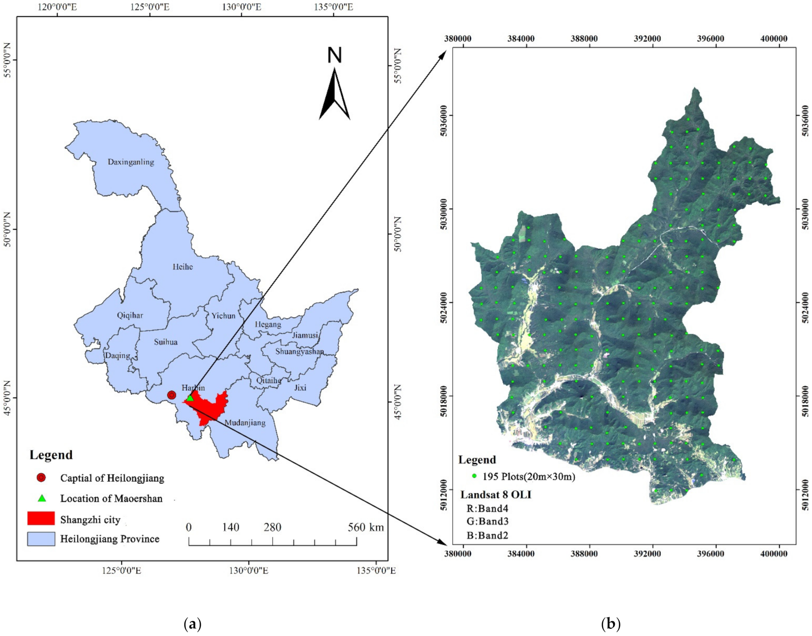
2.1. Study Area
2.2. Data Collection
2.2.1. Remotely Sensed Data
2.2.2. Reference Data
2.3. Methods
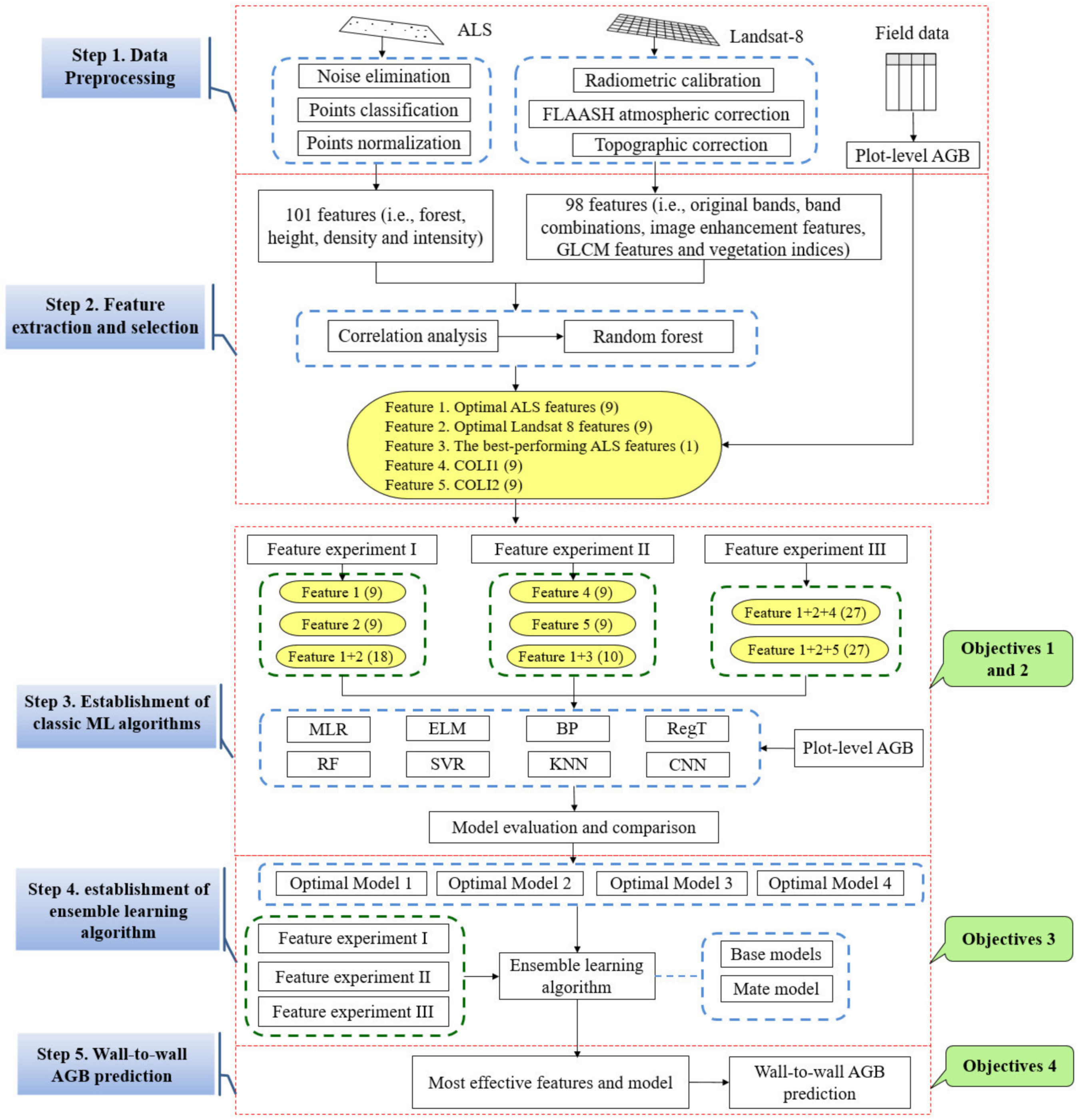
2.3.1. Preprocessing of Remotely Sensed Data
2.3.2. Feature Extraction and Selection
- Feature Extraction
- Feature Selection
2.3.3. Classic Machine Learning Algorithms
- ELM
- BP
- RegT and RF
- SVR
- KNN
- CNN
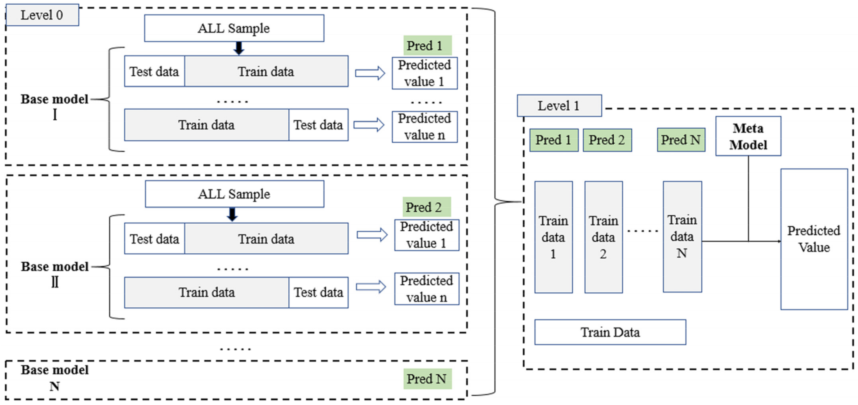
2.3.4. Ensemble Learning Algorithms
2.3.5. Model Evaluation
3. Results
3.1. Feature Selection
3.2. Performance of Classic Machine Learning Algorithms
3.2.1. Experiment I
3.2.2. Experiment II
3.2.3. Experiment III
3.3. Performance of Ensemble Learning Algorithms
3.3.1. Experiment I
3.3.2. Experiment II
3.3.3. Experiment III
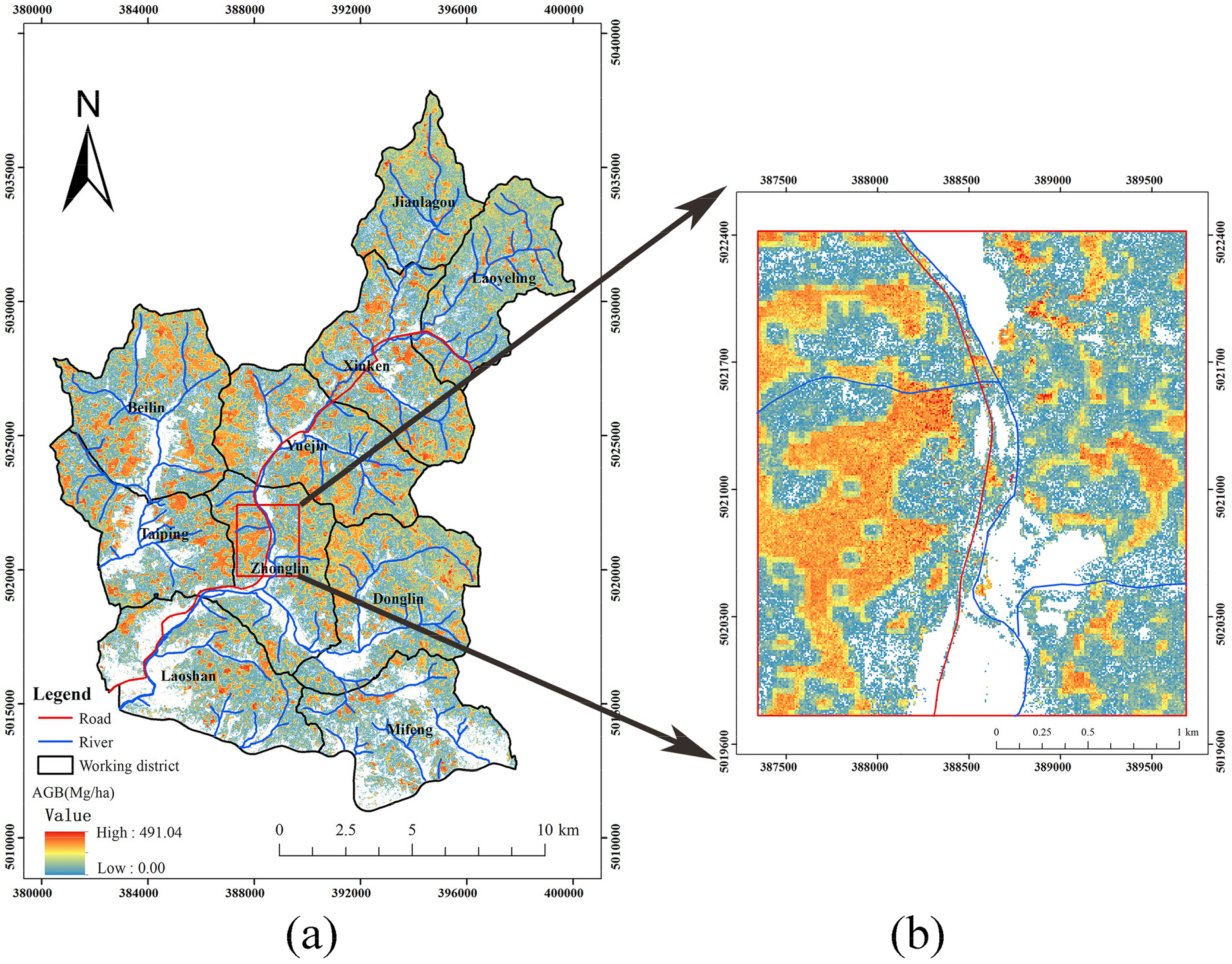
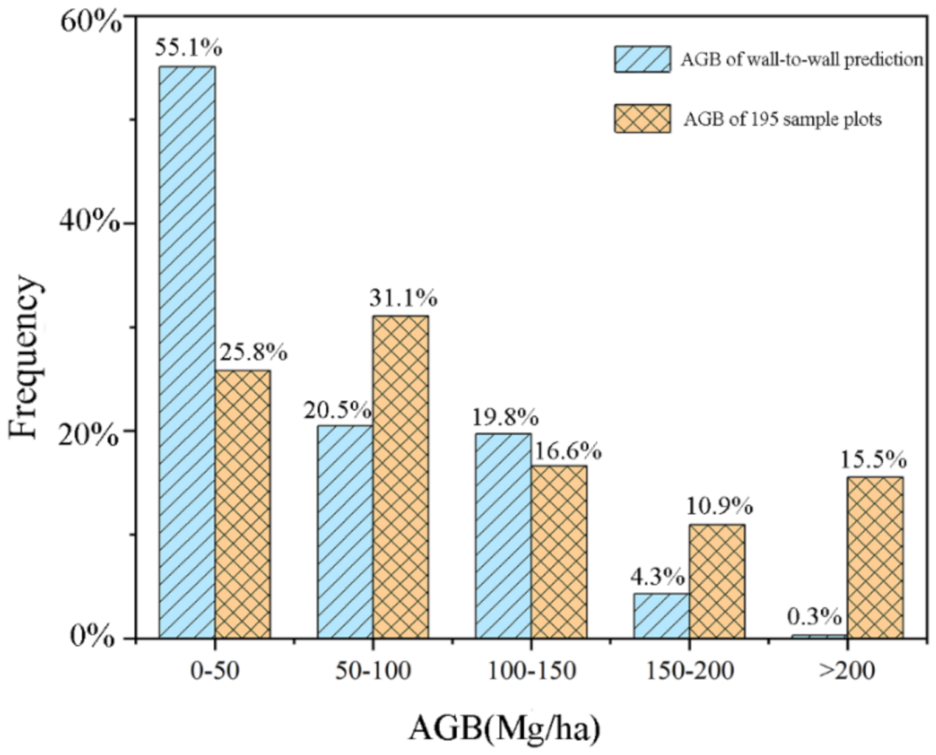
3.4. Wall-to-Wall AGB Predictions
4. Discussion
4.1. AGB Estimation Using Different Features
4.2. AGB Estimation Using Machine Learning Algorithms
4.3. Comparison of Estimated Forest AGB and Current Publications
4.4. Limitations and Recommendations
5. Conclusions
Author Contributions
Funding
Institutional Review Board Statement
Informed Consent Statement
Data Availability Statement
Conflicts of Interest
Appendix A

| Feature Group | Feature Name | Feature Descriptions [111] |
|---|---|---|
| Forest features 1 (3 features) | CC | Canopy cover: CC = Nveg/N |
| G | Gap fraction: G = N’/N | |
| LAI | Leaf area index: | |
| Elevation features (46 features) 2 | elev_AAD | Average absolute deviation of elevation: |
| elev_CRR | Canopy relief ratio of elevation: ( − Zmin)/(Zmax + Zmin) | |
| elev_AIH_ith | The cumulative height of i% points in each pixel is the AIH of the pixel, i = 1%, 5%, 10%, 20%, 25%, 30%, 40%, 50%, 60%, 70%, 75%, 80%, 90%, 95%, 99% | |
| elev_AIH_IQ | AIH interquartile distance: AIH75%–AIH25% | |
| elev_GM_2 | Generalized means for the 2nd power: | |
| elev_GM_3 | Generalized means for the 3rd power: | |
| elev_cv | Coefficient of variation of elevation: Zstd/×100% | |
| elev_IQ | Elevation percentile interquartile distance: Elev75%–Elev25% | |
| elev_kurt | Kurtosis of elevation | |
| elev_MMAD | Median of median absolute deviation of elevation | |
| elev_max | Maximum of elevation | |
| elev_min | Minimum of elevation | |
| elev_mean | Mean of elevation | |
| elev_med | Median of elevation | |
| elev_per_ith | ith elevation percentiles, i = 1%, 5%, 10%, 20%, 25%, 30%, 40%, 50%, 60%, 70%, 75%, 80%, 90%, 95%, 99% | |
| elev_skew | Skewness of elevation | |
| elev_std | Standard deviation of elevation | |
| elev_var | Variance of elevation | |
| Density features (10 features) | density_ith | The proportion of returns in ith height interval, i = 1–10 |
| Intensity features (42 features) 3 | int_AAD | Average absolute deviation of intensity: |
| int_cv | Coefficient of variation of intensity: Istd/×100% | |
| int_AII_ith | The cumulative intensity of X% points in each pixel is the AII of the pixel, i = 1%, 5%, 10%, 20%, 25%, 30%, 40%, 50%, 60%, 70%, 75%, 80%, 90%, 95%, 99% | |
| int_kurt | Kurtosis of intensity | |
| int_MMAD | Median of median absolute deviation of intensity | |
| int_max | Maximum of intensity | |
| int_min | Minimum of intensity | |
| int_mean | Mean of intensity | |
| int_med | Median of intensity | |
| int_per_ith | ith intensity percentiles, i = 1%, 5%, 10%, 20%, 25%, 30%, 40%, 50%, 60%, 70%, 75%, 80%, 90%, 95%, 99% | |
| int_skew | Skewness of intensity | |
| int_std | Standard deviation of intensity | |
| int_var | Variance of intensity | |
| Int_IQ | Intensity percentile interquartile distance: Int75%–Int25% |
| Feature Group | Feature Name | Feature Descriptions |
|---|---|---|
| Original bands (7 features) | Bi 1 | Band1–7 of Landsat 8 OLI image |
| Band combination (10 features) | Albedo | 0.246 B2 + 0.146 B3 + 0.191∙B4 + 0.304∙B5 + 0.105∙B6 + 0.008∙B7 [112] |
| B4/Albedo | B4/(0.246∙B2 + 0.146∙B3 + 0.191∙B4 + 0.304∙B5 + 0.105∙B6 + 0.008∙B7) [112,113] | |
| B24 | B2/B4 [113] | |
| B74 | B7/B4 [113] | |
| B76 | B7/ B6 [113] | |
| B547 | B5∙B4/B7 [113] | |
| B65 | B6/B5 [113] | |
| B345 | B3∙B4/B5 [113] | |
| B53 | B5/B3 [113] | |
| VIS234 | B2 + B3 + B4 [113] | |
| GLCM features 2 (56 features) | Mean_Bi | Mean of each band |
| Var_Bi | Variance of each band | |
| Hom_Bi | Homogeneity of each band | |
| Cont_Bi | Contrast of each band | |
| Diss_Bi | Dissimilarity of each band | |
| Entr_Bi | Entropy of each band | |
| Sec_Bi | Second moment of each band | |
| Corr_Bi | Correlation of each band | |
| Image enhancement features (10 features) | Bright | Brightness from tasseled cap transformation: 0.3521∙B2 + 0.3899∙B3 + 0.3825∙B4 + 0.6985∙B5 + 0.2343∙B6 + 0.1867∙B7 [114] |
| Green | Greenness from tasseled cap transformation: −0.3301∙B2−0.3455∙B3−0.4508∙B4 + 0.6970∙B5−0.0448∙B6−0.2840∙B7 [114] | |
| Wet | Wetness from tasseled cap transformation: 0.2651∙B2 + 0.2367∙B3 + 0.1296∙B4 + 0.059∙B5−0.7506∙B6−0.5386∙B7 [114] | |
| PC1 | The first principal component from principal component analysis (PCA): 0.111∙B3 + 0.870∙B5 + 0.423∙B6 + 0.192∙B7 | |
| PC2 | The second principal component from PCA: 0.198∙B1 + 0.217∙B2 + 0.267∙B3 + 0.376∙B4−0.436∙B5 + 0.430∙B6 + 0.571∙B7 | |
| PC3 | The third principal component from PCA: 0.295∙B1 + 0.324∙B2 + 0.398∙B3 + 0.473∙B4 + 0.183∙B5−0.615∙B6−0.12∙B7 | |
| MNF1 | The first band of minimum noise fraction rotation (MNF): −0.2632∙B1−0.3528∙B2−0.0737∙B3−0.0618∙B4−0.7457∙B5 −0.4898∙B6 + 0.031∙B7 | |
| MNF2 | The second band of MNF: −0.0441∙B1−0.0781∙B2 − 0.1869∙B3 − 0.0389∙B4 − 0.7523∙B5 − 0.4280∙B6 − 0.4542∙B7 | |
| MNF3 | The third band of MNF: −0.2387∙B1 − 0.2230∙B2 + 0.0947∙B3 − 0.0195∙B4 + 0.5277∙B5 + 0.7731∙B6 − 0.0885∙B7 | |
| MNF4 | The fourth band of MNF: 0.0199∙B1 − 0.00013∙B2 − 0.01021∙B3 − 0.1027∙B4 − 0.4377∙B5 − 0.69145∙B6 − 0.565∙B7 | |
| Vegetation indices (15 features) | NDVI | Normalized vegetation index 1: (B5 − B4)/(B5 + B4) [113] |
| RVI | Ratio vegetation index: B5/B4 [113] | |
| DVI | Difference vegetation index: B5 − B4 [113] | |
| EVI | Enhanced vegetation index: 2.5∙(B5 − B4)/(B5 + 6∙B4 − 7.5∙B2 + 1) [113] | |
| MSAVI | Modified soil-adjusted vegetation index: [(B5 − B4)/(B5 + B4 + L)]∙(1 + L) 3 [115] | |
| ARVI | Atmospherically resistant vegetation index: (B5 − 2∙B4 + B2)/(B5 + 2∙B4 − B2) [113] | |
| TVI | Triangular vegetation index: [113] | |
| PVI | Perpendicular vegetation index: [113] | |
| MSR | [113] | |
| SLAVI | Specific leaf area vegetation index: B5/(B4 + B7) [113] | |
| MVI5 | Moisture vegetation index 1: (B5 + B4 − B2)/(B5 + B4 + B2) [116] | |
| MVI7 | Moisture vegetation index 2: (B5 − B7)/(B5 + B7) [116] | |
| NLI | [113] | |
| RDVI | [113] | |
| ND563 | Normalized difference vegetation index 2: (B5 + B6 − B3)/(B5 + B6 + B3) [113] |
References
- Wang, C. Biomass allometric equations for 10 co-occurring tree species in Chinese temperate forests. For. Ecol. Manag. 2006, 222, 9–16. [Google Scholar] [CrossRef]
- Yu, D.; Zhou, L.; Zhou, W.; Ding, H.; Wang, Q.; Wang, Y.; Wu, X.; Dai, L. Forest management in northeast China: History, problems, and challenges. Environ. Manag. 2011, 48, 1122–1135. [Google Scholar] [CrossRef] [PubMed]
- Zhang, P.; Shao, G.; Zhao, G.; Le Master, D.C.; Parker, G.R.; Dunning, J.B., Jr.; Li, Q. China’s forest policy for the 21st century. Science 2000, 288, 2135–2136. [Google Scholar] [CrossRef] [Green Version]
- Zhu, J.; Liu, S. Conception of secondary forest and its relation to ecological disturbance degree. Chin. J. Ecol. 2007, 26, 1085–1093. (In Chinese) [Google Scholar]
- Yang, K.; Zhu, J.; Zhang, M.; Yan, Q.; Sun, O. Soil microbial biomass carbon and nitrogen in forest ecosystems of northeast China: A comparison between natural secondary forest and larch plantation. J. Plant. Ecol. 2010, 3, 175–182. [Google Scholar] [CrossRef]
- CEOS Land Product Validation Subgroup. Available online: https://lpvs.gsfc.nasa.gov/AGB/AGB_home.html (accessed on 29 July 2021).
- Vashum, K.T.; Jayakumar, S. Methods to estimate above-ground biomass and carbon stock in natural forests—A review. J. Ecosyst. Ecography 2012, 2, 116. [Google Scholar] [CrossRef]
- Dong, L.; Zhang, L.; Li, F. Developing two additive biomass equations for three coniferous plantation species in northeast China. Forests 2016, 7, 136. [Google Scholar] [CrossRef] [Green Version]
- Bond-Lamberty, B.; Wang, C.; Gower, S.T. Aboveground and belowground biomass and sapwood area allometric equations for six boreal tree species of northern Manitoba. Can. J. For. Res. 2002, 32, 1441–1450. [Google Scholar] [CrossRef]
- Brown, S.; Gillespie, A.R.; Lugo, A.E. Biomass estimation methods for tropical forests with applications to forest inventory data. For. Sci. 1989, 35, 881–902. [Google Scholar]
- Nelson, B.W.; Mesquita, R.; Pereira, J.L.; de Souza, S.G.A.; Batista, G.T.; Couto, L.B. Allometric regressions for improved estimate of secondary forest biomass in the central Amazon. For. Ecol. Manag. 1999, 117, 149–167. [Google Scholar] [CrossRef]
- Chung-Wang, X.; Ceulemans, R. Allometric relationships for below- and above-ground biomass of young Scots pines. For. Ecol. Manag. 2004, 203, 177–186. [Google Scholar]
- Chave, J.; Riéra, B.; Dubois, M. Estimation of biomass in a neotropical forest of French Guiana: Spatial and temporal variability. J. Trop. Ecol. 2001, 17, 79–96. [Google Scholar] [CrossRef] [Green Version]
- Fang, J.; Chen, A.; Peng, C.; Zhao, S.; Ci, L. Changes in forest biomass carbon storage in china between 1949 and 1998. Science 2001, 292, 2320–2322. [Google Scholar] [CrossRef]
- Lu, D.; Chen, Q.; Wang, G.; Liu, L.; Li, G.; Moran, E. A survey of remote sensing-based aboveground biomass estimation methods in forest ecosystems. Int. J. Digit. Earth 2014, 9, 63–105. [Google Scholar] [CrossRef]
- White, J.; Coops, N.; Scott, N. Estimates of New Zealand forest and scrub biomass from the 3-PG model. Ecol. Model. 2000, 131, 175–190. [Google Scholar] [CrossRef]
- Chen, Q. LiDAR remote sensing of vegetation biomass. In Remote Sensing of Natural Resources; CRC PRESS: Boca Raton, FL, USA, 2014. [Google Scholar]
- Jenkins, J.C.; Birdsey, R.A.; Pan, Y. Biomass and NPP estimation for the mid-Atlantic region (USA) using plot-level forest in-ventory data. Ecol. Appl. 2001, 11, 1174–1193. [Google Scholar] [CrossRef]
- Cao, L.; Pan, J.; Li, R.; Li, J.; Li, Z. Integrating airborne LiDAR and optical data to estimate forest aboveground biomass in arid and semi-arid regions of China. Remote Sens. 2018, 10, 532. [Google Scholar] [CrossRef] [Green Version]
- Endres, A.; Mountrakis, G.; Jin, H.; Zhuang, W.; Manakos, I.; Wiley, J.J.; Beier, C.M. Relative importance analysis of Landsat, waveform LIDAR and PALSAR inputs for deciduous biomass estimation. Eur. J. Remote Sens. 2016, 49, 795–807. [Google Scholar] [CrossRef] [Green Version]
- Laurin, G.V.; Chen, Q.; Lindsell, J.; Coomes, D.A.; Del Frate, F.; Guerriero, L.; Pirotti, F.; Valentini, R. Above ground biomass estimation in an African tropical forest with lidar and hyperspectral data. ISPRS J. Photogramm. Remote Sens. 2014, 89, 49–58. [Google Scholar] [CrossRef]
- Foody, G.M.; Boyd, D.; Cutler, M. Predictive relations of tropical forest biomass from Landsat TM data and their transferability between regions. Remote Sens. Environ. 2003, 85, 463–474. [Google Scholar] [CrossRef]
- Myneni, R.B.; Dong, J.; Tucker, C.J.; Kaufmann, R.K.; Kauppi, P.E.; Liski, J.; Zhou, L.; Alexeyev, V.; Hughes, M.K. A large carbon sink in the woody biomass of Northern forests. Proc. Natl. Acad. Sci. USA 2001, 98, 14784–14789. [Google Scholar] [CrossRef] [Green Version]
- Thenkabail, P.S.; Enclona, E.A.; Ashton, M.S.; Legg, C.; De Dieu, M.J. Hyperion, IKONOS, ALI and ETM plus sensors in the study of African rainforests. Remote Sens. Environ. 2004, 90, 23–43. [Google Scholar] [CrossRef]
- Clark, D.B.; Read, J.M.; Clark, M.L.; Cruz, A.M.; Dotti, M.F.; Clark, D.A. Application of 1-m and 4-m resolution satellite data to ecological studies of tropical rain forests. Ecol. Appl. 2004, 14, 61–74. [Google Scholar] [CrossRef]
- Gasparri, N.I.; Parmuchi, M.G.; Bono, J.; Karszenbaum, H.; Montenegro, C.L. Assessing multi-temporal Landsat 7 ETM + images for estimating above-ground biomass in subtropical dry forests of Argentina. J. Arid. Environ. 2010, 74, 1262–1270. [Google Scholar] [CrossRef]
- Gömez, C.; White, J.C.; Wulder, M.A.; Alejandro, P. Historical forest biomass dynamics modelled with Landsat spectral tra-jectories. ISPRS J. Photogramm. Remote Sens. 2014, 93, 14–28. [Google Scholar] [CrossRef] [Green Version]
- Dube, T.; Mutanga, O. Investigating the robustness of the new Landsat-8 Operational Land Imager derived texture metrics in estimating plantation forest aboveground biomass in resource constrained areas. ISPRS J. Photogramm. Remote Sens. 2015, 108, 12–32. [Google Scholar] [CrossRef]
- Kelsey, K.C.; Neff, J.C. Estimates of aboveground biomass from texture analysis of landsat imagery. Remote Sens. 2014, 6, 6407–6422. [Google Scholar] [CrossRef] [Green Version]
- Dube, T.; Mutanga, O. Evaluating the utility of the medium-spatial resolution Landsat 8 multispectral sensorin quantifying aboveground biomass in uMgeni catchment, South Africa. ISPRS J. Photogramm. Remote Sens. 2015, 101, 36–46. [Google Scholar] [CrossRef]
- Loveland, T.R.; Irons, J.R. Landsat 8: The plans, the reality, and the legacy. Remote Sens Environ. 2016, 185, 1–6. [Google Scholar] [CrossRef] [Green Version]
- Lu, D. Aboveground biomass estimation using Landsat TM data in the Brazilian Amazon. Int. J. Remote Sens. 2005, 26, 2509–2525. [Google Scholar] [CrossRef]
- Zhao, P.; Lu, D.; Wang, G.; Wu, C.; Huang, Y.; Yu, S. Examining spectral reflectance saturation in Landsat imagery and cor-responding solutions to improve forest aboveground biomass estimation. Remote Sens. 2016, 8, 469. [Google Scholar] [CrossRef] [Green Version]
- Steininger, M.K. Satellite estimation of tropical secondary forest above-ground biomass: Data from Brazil and Bolivia. Int. J. Remote Sens. 2000, 21, 1139–1157. [Google Scholar] [CrossRef]
- Lucas, R.M.; Held, A.A.; Phinn, S.R.; Saatchi, S. Tropical forests. In Remote Sensing for Natural Resource Management and En-vironmental Monitoring, 3rd ed.; Ustin, S.D., Ed.; John Wiley & Sons, Inc.: Hoboken, NJ, USA, 2004; Volume 3, pp. 239–315. [Google Scholar]
- Le Toan, T.; Quegan, S.; Woodward, I.; Lomas, M.; Delbart, N.; Picard, G. Relating radar remote sensing of biomass to mod-elling of forest carbon budgets. Clim. Chang. 2004, 67, 379–402. [Google Scholar] [CrossRef]
- Waring, R.H.; Way, J.; Hunt, E.R.; Morrissey, L.; Ranson, K.J.; Weishampel, J.F.; Oren, R.; Franklin, S.E. Imaging radar for ecosystem studies. BioScience 1995, 45, 715–723. [Google Scholar] [CrossRef]
- Zolkos, S.; Goetz, S.; Dubayah, R. A meta-analysis of terrestrial aboveground biomass estimation using lidar remote sensing. Remote Sens. Environ. 2012, 128, 289–298. [Google Scholar] [CrossRef]
- Gonzalez, P.; Asner, G.P.; Battles, J.J.; Lefsky, M.A.; Waring, K.M.; Palace, M. Forest carbon densities and uncertainties from Lidar, QuickBird, and field measurements in California. Remote Sens. Environ. 2010, 114, 1561–1575. [Google Scholar] [CrossRef]
- Means, J.E.; Acker, S.A.; Harding, D.J.; Blair, J.B.; Lefsky, M.A.; Cohen, W.B.; Harmon, M.E.; McKee, W.A. Use of large-footprint scanning airborne lidar to estimate forest stand characteristics in the western cascades of Oregon. Remote Sens. Environ. 1999, 67, 298–308. [Google Scholar] [CrossRef]
- Lu, D.; Chen, Q.; Wang, G.; Moran, E.; Batistella, M.; Zhang, M.; Laurin, G.V.; Saah, D. Aboveground forest biomass estima-tion with Landsat and Lidar data and uncertainty analysis of the estimates. Int. J. For. Res. 2012, 2012, 250–265. [Google Scholar]
- Mauya, E.W.; Ene, L.T.; Bollandsås, O.M.; Gobakken, T.; Naesset, E.; Malimbwi, R.E.; Zahabu, E. Modelling aboveground forest biomass using airborne laser scanner data in the miombo woodlands of Tanzania. Carbon Balance Manag. 2015, 10, 28. [Google Scholar] [CrossRef] [Green Version]
- Gleason, C.J.; Im, J. Forest biomass estimation from airborne LiDAR data using machine learning approaches. Remote Sens. Environ. 2012, 125, 80–91. [Google Scholar] [CrossRef]
- Ioki, K.; Tsuyuki, S.; Hirata, Y.; Phua, M.H.; Wong, W.V.C.; Ling, Z.Y.; Saito, H.; Takao, G. Estimating above-ground bio-mass of tropical rainforest of different degradation levels in Northern Borneo using airborne LiDAR. For. Ecol. Manag. 2014, 328, 335–341. [Google Scholar] [CrossRef]
- Hansen, E.H.; Gobakken, T.; Bollandsås, O.M.; Zahabu, E.; Næsset, E. Modeling aboveground biomass in dense tropical submontane rainforest using airborne laser scanner data. Remote Sens. 2015, 7, 788–807. [Google Scholar] [CrossRef] [Green Version]
- Magdon, P.; González-Ferreiro, E.; Pérez-Cruzado, C.; Purnama, E.S.; Sarodja, D.; Kleinn, C. Evaluating the potential of ALS data to increase the efficiency of aboveground biomass estimates in tropical peat–swamp forests. Remote Sens. 2018, 10, 1344. [Google Scholar] [CrossRef] [Green Version]
- Adhikari, H.; Heiskanen, J.; Siljander, M.; Maeda, E.; Heikinheimo, V.; Pellikka, P.K.E. Determinants of aboveground bio-mass across an Afromontane landscape mosaic in Kenya. Remote Sens. 2017, 9, 827. [Google Scholar] [CrossRef] [Green Version]
- Zhang, L.; Shao, Z.; Liu, J.; Cheng, Q. Deep learning based retrieval of forest aboveground biomass from combined LiDAR and landsat 8 data. Remote Sens. 2019, 11, 1459. [Google Scholar] [CrossRef] [Green Version]
- Clark, M.L.; Roberts, D.A.; Ewel, J.J.; Clark, D.B. Estimation of tropical rain forest aboveground biomass with small-footprint lidar and hyperspectral sensors. Remote Sens. Environ. 2011, 115, 2931–2942. [Google Scholar] [CrossRef]
- Egberth, M.; Nyberg, G.; Næsset, E.; Gobakken, T.; Mauya, E.; Malimbwi, R.; Katani, J.; Chamuya, N.; Bulenga, G.; Olsson, H. Combining airborne laser scanning and Landsat data for statistical modeling of soil carbon and tree biomass in Tanzanian Miombo woodlands. Carbon Balance Manag. 2017, 12, 8. [Google Scholar] [CrossRef] [PubMed] [Green Version]
- Heiskanen, J.; Adhikari, H.; Piiroinen, R.; Packalen, P.; Pellikka, P.K. Do airborne laser scanning biomass prediction models benefit from Landsat time series, hyperspectral data or forest classification in tropical mosaic landscapes? Int. J. Appl. Earth Obs. Geoinf. 2019, 81, 176–185. [Google Scholar] [CrossRef]
- Phua, M.H.; Johari, S.A.; Wong, O.C.; Ioki, K.; Mahali, M.; Nilus, R.; Coomes, D.A.; Maycock, C.R.; Hashim, M. Synergistic use of Landsat 8 OLI image and airborne LiDAR data for above-ground biomass estimation in tropical lowland rainforests. For. Ecol. Manag. 2017, 406, 163–171. [Google Scholar] [CrossRef]
- Li, S.; Quackenbush, L.J.; Im, J. Airborne lidar sampling strategies to enhance forest aboveground biomass estimation from landsat imagery. Remote Sens. 2019, 11, 1906. [Google Scholar] [CrossRef] [Green Version]
- Li, Y.; Li, C.; Li, M.; Liu, Z. Influence of variable selection and forest type on forest aboveground biomass estimation using machine learning algorithms. Forests 2019, 10, 1073. [Google Scholar] [CrossRef] [Green Version]
- Blackard, J.A.; Finco, M.V.; Helmer, E.H.; Holden, G.R.; Hoppous, M.L.; Jacobs, D.M.; Lister, A.J.; Moisen, G.G.; Nelson, M.D.; Riemann, R.; et al. Mapping US forest biomass using nationwide forest inventory data and moderate resolution information. Remote Sens. Environ. 2008, 112, 1658–1677. [Google Scholar] [CrossRef]
- Houghton, R.A.; Lawrence, K.T.; Hackler, J.L.; Brown, S. The spatial distribution of forest biomass in the Brazilian amazon: A comparison of estimates. Glob. Chang. Biol. 2001, 7, 731–746. [Google Scholar] [CrossRef]
- Tan, K.; Piao, S.; Peng, C.; Fang, J. Satellite-based estimation of biomass carbon stocks for northeast China’s forests between 1982 and 1999. For. Ecol. Manag. 2007, 240, 114–121. [Google Scholar] [CrossRef]
- Chen, L.; Ren, C.; Zhang, B.; Wang, Z.; Xi, Y. Estimation of forest above-ground biomass by geographically weighted regres-sion and machine learning with sentinel imagery. Forests 2018, 9, 582. [Google Scholar] [CrossRef] [Green Version]
- Lim, K.S.; Treitz, P.M. Estimation of above ground forest biomass from airborne discrete return laser scanner data using canopy-based quantile estimators. Scand. J. For. Res. 2004, 19, 558–570. [Google Scholar] [CrossRef] [Green Version]
- Zhao, K.; Popescu, S.; Nelson, R. Lidar remote sensing of forest biomass: A scale-invariant estimation approach using air-borne lasers. Remote Sens. Environ. 2009, 113, 182–196. [Google Scholar] [CrossRef]
- Kulawardhana, R.W.; Popescu, S.; Feagin, R. Fusion of lidar and multispectral data to quantify salt marsh carbon stocks. Remote Sens. Environ. 2014, 154, 345–357. [Google Scholar] [CrossRef]
- Li, W.; Niu, Z.; Wang, C.; Huang, W.; Chen, H.; Gao, S.; Li, D.; Muhammad, S. Combined use of airborne LiDAR and satellite GF-1 data to estimate leaf area index, height, and aboveground biomass of maize during peak growing season. IEEE J. Sel. Top. Appl. Earth Obs. Remote Sens. 2015, 8, 4489–4501. [Google Scholar] [CrossRef]
- Verrelst, J.; Camps-Valls, G.; Muñoz-Marí, J.; Rivera, J.P.; Veroustraete, F.; Clevers, J.G.P.W.; Moreno, J. Optical remote sensing and the retrieval of terrestrial vegetation bio-geophysical properties—A review. ISPRS J. Photogramm. 2015, 108, 273–290. [Google Scholar] [CrossRef]
- Asner, G.P.; Hughes, R.F.; Varga, T.A.; Knapp, D.E.; Kennedy-Bowdoin, T. Environmental and biotic controls over above-ground biomass throughout a tropical rain forest. Ecosystems 2009, 12, 261–278. [Google Scholar] [CrossRef]
- Lucas, R.M.; Cronin, N.; Lee, A.; Moghaddam, M.; Witte, C.; Tickle, P. Empirical relationships between AIRSAR backscatter and LiDAR-derived forest biomass, Queensland, Australia. Remote Sens. Environ. 2006, 100, 407–425. [Google Scholar] [CrossRef]
- Patenaude, G.; Hill, R.; Milne, R.; Gaveau, D.; Briggs, B.; Dawson, T. Quantifying forest above ground carbon content using LiDAR remote sensing. Remote Sens. Environ. 2004, 93, 368–380. [Google Scholar] [CrossRef]
- St-Onge, B.; Hu, Y.; Vega, C. Mapping the height and above-ground biomass of a mixed forest using lidar and stereo Ikonos images. Int. J. Remote Sens. 2008, 29, 1277–1294. [Google Scholar] [CrossRef]
- Xie, Y.; Sha, Z.; Yu, M.; Bai, Y.; Zhang, L. A comparison of two models with Landsat data for estimating above ground grassland biomass in Inner Mongolia, China. Ecol. Model. 2009, 220, 1810–1818. [Google Scholar] [CrossRef]
- Su, Y.; Guo, Q.; Xue, B.; Hu, T.; Alvarez, O.; Tao, S.; Fang, J. Spatial distribution of forest aboveground biomass in China: Estimation through combination of spaceborne lidar, optical imagery, and forest inventory data. Remote Sens. Environ. 2016, 173, 187–199. [Google Scholar] [CrossRef] [Green Version]
- Li, M.; Im, J.; Quackenbush, L.J.; Liu, T. Forest biomass and carbon stock quantification using airborne LiDAR data: A case study over huntington wildlife forest in the adirondack park. IEEE J. Sel. Top. Appl. Earth Obs. Remote Sens. 2014, 7, 3143–3156. [Google Scholar] [CrossRef]
- Ou, G.; Li, C.; Lv, Y.; Wei, A.; Xiong, H.; Xu, H.; Wang, G. Improving aboveground biomass estimation of pinus densata forests in yunnan using landsat 8 imagery by incorporating age dummy variable and method comparison. Remote Sens. 2019, 11, 738. [Google Scholar] [CrossRef] [Green Version]
- Serrano, P.M.L.; López-Sánchez, C.A.; Álvarez-González, J.G.; García-Gutiérrez, J. A Comparison of machine learning techniques applied to landsat-5 tm spectral data for biomass estimation. Can. J. Remote Sens. 2016, 42, 690–705. [Google Scholar] [CrossRef]
- Dong, L.; Du, H.; Han, N.; Li, X.; Zhu, D.; Mao, F.; Zhang, M.; Zheng, J.; Liu, H.; Huang, Z.; et al. Application of convolutional neural network on lei bamboo Above-Ground-Biomass (AGB) estimation using worldview-2. Remote Sens. 2020, 12, 958. [Google Scholar] [CrossRef] [Green Version]
- Luo, M.; Wang, Y.; Xie, Y.; Zhou, L.; Qiao, J.; Qiu, S.; Sun, Y. Combination of feature selection and catboost for prediction: The first application to the estimation of aboveground biomass. Forests 2021, 12, 216. [Google Scholar] [CrossRef]
- Sonobe, R.; Yamaya, Y.; Tani, H.; Wang, X.; Kobayashi, N.; Mochizuki, K. Crop classification from Sentinel-2-derived vege-tation indices using ensemble learning. J. Appl. Remote Sens. 2018, 12, 26019. [Google Scholar] [CrossRef] [Green Version]
- Breiman, L. Random Forests. Mach Learn. 2001, 45, 5–23. [Google Scholar] [CrossRef] [Green Version]
- Zeng, N.; Ren, X.; He, H.; Zhang, L.; Zhao, D.; Ge, R.; Li, P.; Niu, Z. Estimating grassland aboveground biomass on the Ti-betan Plateau using a random forest algorithm. Ecol. Indic. 2019, 102, 479–487. [Google Scholar] [CrossRef]
- Wolpert, D.H. Stacked generalization. Neural Netw. 1992, 5, 241–259. [Google Scholar] [CrossRef]
- Jiang, F.; Zhao, F.; Ma, K.; Li, D.; Sun, H. Mapping the forest canopy height in northern china by synergizing ICESat-2 with sentinel-2 using a stacking algorithm. Remote Sens. 2021, 13, 1535. [Google Scholar] [CrossRef]
- Dong, L. Study on the Compatible Modles of Tree Biomass for Main Species in Heilongjiang Province. Master’s Thesis, Northeast Forestry University, Harbin, Heilongjiang, China, 2012. (In Chinese). [Google Scholar]
- Li, X.; Guo, Q.; Wang, X.; Zheng, H. Allometry of understory tree species in a natural secondary forest in northeast China. Sci. Silvae Sin. 2010, 46, 22–32. (In Chinese) [Google Scholar]
- Zhao, X.; Guo, Q.; Su, Y.; Xue, B. Improved progressive TIN densification filtering algorithm for airborne LiDAR data in for-ested areas. ISPRS J. Photogramm. 2016, 117, 79–91. [Google Scholar] [CrossRef] [Green Version]
- Soenen, S.A.; Peddle, D.R.; Coburn, C.A. SCS + C: A modified Sun-canopy-sensor topographic correction in forested terrain. IEEE T. Geosci. Remote 2005, 43, 2148–2159. [Google Scholar] [CrossRef]
- Soenen, S.A.; Peddle, D.R.; Hall, R.J.; Coburn, C.A.; Hall, F.G. Estimating aboveground forest biomass from canopy reflectance model inversion in mountainous terrain. Remote Sens Environ. 2010, 114, 1325–1337. [Google Scholar] [CrossRef]
- Jennings, S.; Brown, N.; Sheil, D. Assessing forest canopies and understorey illumination: Canopy closure, canopy cover and other measures. Forestry 1999, 72, 59–74. [Google Scholar] [CrossRef]
- Chen, J.; Black, T. Measuring leaf area index of plant canopies with branch architecture. Agric. For. Meteorol. 1991, 57, 1–12. [Google Scholar] [CrossRef]
- Ou, G.; Lv, Y.; Xu, H.; Wang, G. Improving forest aboveground biomass estimation of pinus densata forest in yunnan of southwest china by spatial regression using Landsat 8 images. Remote Sens. 2019, 11, 2750. [Google Scholar] [CrossRef] [Green Version]
- Huang, G.-B.; Zhu, Q.-Y.; Siew, C.-K. Extreme learning machine: Theory and applications. Neurocomputing 2006, 70, 489–501. [Google Scholar] [CrossRef]
- Rumelhart, D.E.; Hinton, G.E.; Williams, R.J. Learning representations by back-propagating errors. Nature 1986, 323, 533–536. [Google Scholar] [CrossRef]
- Zhu, Y.; Liu, K.; Liu, L.; Wang, S.; Liu, H. Retrieval of mangrove aboveground biomass at the individual species level with worldview-2 images. Remote Sens. 2015, 7, 12192–12214. [Google Scholar] [CrossRef] [Green Version]
- LeCun, Y.; Bengio, Y. Convolutional networks for images, speech, and time series. In The Handbook of Brain Theory and Neural Network; MIT Press: Cambridge, MA, USA, 1995; Volume 3361, pp. 1–14. [Google Scholar]
- Chen, T.; Guestrin, C. XGBoost: A scalable tree boosting system. In Proceedings of the 22nd ACM SIGKDD International Conference on Knowledge Discovery and Data Mining, San Francisco, CA, USA, 13–17 August 2016; Association for Computing Machinery: New York, NY, USA, 2016; pp. 785–794. [Google Scholar]
- Feng, L.; Li, Y.; Wang, Y.; Du, Q. Estimating hourly and continuous ground-level PM2.5 concentrations using an ensemble learning algorithm: The ST-stacking model. Atmos. Environ. 2019, 223, 117242. [Google Scholar] [CrossRef]
- Wen, L.; Hughes, M. Coastal wetland mapping using ensemble learning algorithms: A comparative study of bagging, boosting and stacking techniques. Remote Sens. 2020, 12, 1683. [Google Scholar] [CrossRef]
- Book, S.A.; Yong, P.H. The trouble with R2. J. Parametr. 2006, 25, 87–114. [Google Scholar] [CrossRef]
- Van Der Meer, F.; Bakker, W.; Scholte, K.; Skidmore, A.; De Jong, S.; Clevers, E.A.; Epema, G. Spatial scale variations in veg-etation indices and above-ground biomass estimates: Implications for MERIS. Int. J. Remote Sens. 2001, 22, 3381–3396. [Google Scholar] [CrossRef]
- Huang, S.; Tang, L.; Hupy, J.P.; Wang, Y.; Shao, G. A commentary review on the use of normalized difference vegetation index (NDVI) in the era of popular remote sensing. J. For. Res. 2020, 32, 1–6. [Google Scholar] [CrossRef]
- Wu, Z.; Dye, D.; Vogel, J.; Middleton, B. Estimating forest and woodland aboveground biomass using active and passive re-mote sensing. Photogramm. Eng. Rem. S. 2016, 82, 271–281. [Google Scholar] [CrossRef]
- Krizhevsky, A.; Sutskever, I.; Hinton, G.E. ImageNet classification with deep convolutional neural networks. Commun. ACM 2017, 60, 84–90. [Google Scholar] [CrossRef]
- Ayrey, E.; Hayes, D.J. The use of three-dimensional convolutional neural networks to interpret LiDAR for forest inventory. Remote Sens. 2018, 10, 649. [Google Scholar] [CrossRef] [Green Version]
- Fricker, G.A.; Ventura, J.D.; Wolf, J.A.; North, M.P.; Davis, F.W.; Franklin, J. A convolutional neural network classifier iden-tifies tree species in mixed-conifer forest from hyperspectral imagery. Remote Sens. 2019, 11, 2326. [Google Scholar] [CrossRef] [Green Version]
- Fassnacht, F.; Hartig, F.; Latifi, H.; Berger, C.; Hernández, J.; Corvalán, P.; Koch, B. Importance of sample size, data type and prediction method for remote sensing-based estimations of aboveground forest biomass. Remote Sens. Environ. 2014, 154, 102–114. [Google Scholar] [CrossRef]
- Yang, L.; Liang, S.; Zhang, Y. A new method for generating a global forest aboveground biomass map from multiple high-level satellite products and ancillary information. IEEE J. Sel. Top. Appl. Earth Obs. Remote Sens. 2020, 13, 2587–2597. [Google Scholar] [CrossRef]
- Guo, Z.; Hu, H.; Li, P.; Li, N.; Fang, J. Spatio-temporal changes in biomass carbon sinks in China’s forests from 1977 to 2008. Sci. China Life Sci. 2013, 56, 661–671. [Google Scholar] [CrossRef] [Green Version]
- Zhang, Y.; Liang, S.; Sun, G. Forest biomass mapping of northeastern china using GLAS and MODIS Data. IEEE J. Sel. Top. Appl. Earth Obs. Remote Sens. 2013, 7, 140–152. [Google Scholar] [CrossRef]
- Sammut, C.; Webb, G.I. (Eds.) Leave-one-out cross-validation. In Encyclopedia of Machine Learning, 2020 ed.; Springer: Boston, MA, USA, 2011. [Google Scholar]
- Réjou-Méchain, M.; Barbier, N.; Couteron, P.; Ploton, P.; Vincent, G.; Herold, M.; Mermoz, S.; Saatchi, S.; Chave, J.; de Bois-sieu, F.; et al. Upscaling forest biomass from field to satellite measurements: Sources of errors and ways to reduce them. Surv. Geophys. 2019, 40, 881–911. [Google Scholar] [CrossRef]
- Xu, Q.; Man, A.; Fredrickson, M.; Hou, Z.; Pitkänen, J.; Wing, B. Quantification of uncertainty in aboveground biomass esti-mates derived from small-footprint airborne LiDAR. Remote Sens. Environ. 2018, 216, 514–528. [Google Scholar] [CrossRef]
- Zhen, Z.; Quackenbush, L.J.; Stehman, S.V.; Zhang, L. Agent-based region growing for individual tree crown delineation from airborne laser scanning (ALS) data. Int. J. Remote Sens. 2015, 36, 1965–1993. [Google Scholar] [CrossRef]
- Zhao, Y.; Hao, Y.; Zhen, Z.; Quan, Y. A region-based hierarchical cross-section analysis for individual tree crown delineation using ALS Data. Remote Sens. 2017, 9, 1084. [Google Scholar] [CrossRef] [Green Version]
- GreenValley International. LiDAR360 V3.2 User Guide; GreenValley International, Ltd.: Beijing, China, 2019. [Google Scholar]
- Olmedo, G.F.; Ortega-Farías, S.; de la Fuente-Sáiz, D.; Fonseca-Luego, D.; Fuentes-Peñailillo, F. water: Tools and functions to es-timate actual evapotranspiration using land surface energy balance models in R. R J. 2016, 8, 352–369. [Google Scholar] [CrossRef] [Green Version]
- Xu, T.; Cao, L.; Shen, X.; She, G. Estimates of subtropical forest biomass based on airborne LiDAR and Landsat 8 OLI data. Chin. J. Plant Ecol. 2015, 39, 309–321. (In Chinese) [Google Scholar]
- Li, B.; Di, C.; Yan, X. Study of derivation of tasseled cap transformation for Landsat 8 OLI images. Sci. Surv. Mapp. 2016, 41, 102–107. (In Chinese) [Google Scholar]
- Qi, J.; Chehbouni, A.; Huete, A.R.; Kerr, Y.H.; Sorooshian, S. A modified soil adjusted vegetation index. Remote Sens. Environ. 1994, 48, 119–126. [Google Scholar] [CrossRef]
- Zhou, L.; Ou, G.; Wang, J.; Xu, H. Light saturation point determination and biomass remote sensing estimation of Pinus kesiya var. langbianensis forest based on spatial regression models. Sci. Silvae Sin. 2020, 56, 38–46. (In Chinese) [Google Scholar]


| Vegetation Types | Latin Names of Species | a | b |
|---|---|---|---|
| Deciduous trees | Acer mono Maxim. | 0.318 | 2.081 |
| Ulmus pumila L. | 0.350 | 1.995 | |
| Populus davidiana Dode | 0.078 | 2.512 | |
| Betula platyphylla | 0.313 | 2.114 | |
| Quercus mongolica Fisch. ex Ledeb. | 0.097 | 2.501 | |
| Tilia mongolica Maxim | 0.083 | 2.422 | |
| Fraxinus mandshurica Rupr./Juglans mandshurica Maxim/Phellodendron amurense Rupr. | 0.268 | 2.118 | |
| Coniferous trees | Larix olgensis Henry | 0.168 | 2.248 |
| Pinus koraiensis Sieb.et Zucc. | 0.082 | 2.426 | |
| Picea asperata Mast. | 0.067 | 2.517 | |
| Larix olgensis Henry 1 | 0.222 | 2.174 | |
| Pinus koraiensis Sieb.et Zucc.1 | 0.206 | 2.117 | |
| Pinus sylvestris var. mongolica Litv. 1 | 0.080 | 2.440 | |
| Understory | Acer ginnala | 0.527 | 2.217 |
| Syringa reticulata var. amurensis | 0.395 | 2.300 | |
| Padus asiatica | 0.090 | 2.696 | |
| Rhamnus yoshinoi | 0.169 | 2.555 | |
| Arbor-like mixed species 2 | 0.182 | 2.487 |
| Experiment | Data Source | Number of Features 1 | Details |
|---|---|---|---|
| I | ALS | 9 | Feature 1: Optimal ALS features |
| Landsat 8 | 9 | Feature 2: Optimal Landsat 8 features | |
| ALS + Landsat 8 | 18 | Feature 1 + 2: Optimal ALS and Landsat 8 features | |
| II | ALS + Landsat 8 | 9 | Feature 4: All COLI1 2 |
| 9 | Feature 5: All COLI2 2 | ||
| 10 | Feature 2 + 3 3: Optimal Landsat 8 features (9) + The best performing ALS feature (1) | ||
| III | ALS + Landsat 8 | 27 | Feature 1 + 2 + 4: Optimal ALS features (9) + Optimal Landsat 8 features (9) + All COLI1 (9) |
| 27 | Feature 1 + 2 + 5: Optimal ALS features (9) + Optimal Landsat 8 features (9) + All COLI2 (9) |
| ALS | Feature Descriptions | Landsat 8 | Feature Descriptions |
|---|---|---|---|
| elev_mean | Mean value of height | MVI5 | (B5 + B4 − B2)/(B5 + B4 + B2) |
| int_AII_5th | The cumulative intensity of 5% points in each pixel | B1 | Band 1 |
| elev_cv | Coefficient of variation of height | B76 | B7/B6 |
| density_7th | The proportion of returns in 7th height interval | B65 | B6/B5 |
| int_max | Max of intensity | B53 | B5/B3 |
| int_AII_40th | The cumulative intensity of 40% points in each pixel | Entr_B5 | Entropy of band 5 |
| int_per_60th | 60% intensity percentile | B2 | Band 2 |
| int_per_80th | 80% intensity percentile | ND563 | (B5 + B6 − B3)∙(B5 + B6 + B3) |
| int_AII_50th | The cumulative intensity of 50% points in each pixel | MVI7 | (B5 − B7)/(B5 + B7) |
| ALS Features | R2 | RMSE | rRMSE | MAE | MAPE | PM |
|---|---|---|---|---|---|---|
| elev_mean | 0.34 | 60.03 | 0.40 | 43.74 | 0.39 | 0.67 |
| int_AII_5th | 0.13 | 68.75 | 0.46 | 51.70 | 0.65 | 0.87 |
| elev_cv | 0.08 | 70.64 | 0.48 | 53.99 | 0.66 | 0.92 |
| density_7th | 0.05 | 71.89 | 0.48 | 53.27 | 0.87 | 0.95 |
| int_max | 0.19 | 66.41 | 0.45 | 49.03 | 0.64 | 0.81 |
| int_AII_40th | 0.20 | 65.97 | 0.44 | 49.85 | 0.63 | 0.80 |
| int_per_60th | 0.17 | 66.89 | 0.45 | 50.68 | 0.64 | 0.83 |
| int_per_80th | 0.17 | 66.94 | 0.45 | 50.51 | 0.66 | 0.83 |
| Features | Algorithm 1 | R2 | RMSE | rRMSE | MAE | MAPE | PM |
|---|---|---|---|---|---|---|---|
| Optimal ALS features (Feature 1) | MLR | 0.31 | 52.76 | 0.37 | 41.09 | 38.37 | 0.67 |
| ELM | 0.31 | 56.79 | 0.40 | 42.61 | 35.49 | 0.69 | |
| BP | 0.28 | 61.01 | 0.42 | 44.37 | 36.01 | 0.71 | |
| RegT | 0.21 | 71.95 | 0.47 | 58.55 | 42.66 | 1.11 | |
| RF | 0.29 | 61.84 | 0.41 | 45.80 | 37.08 | 0.72 | |
| SVR | 0.40 | 57.84 | 0.38 | 39.32 | 32.35 | 0.66 | |
| KNN | 0.31 | 60.95 | 0.4 | 45.21 | 35.36 | 0.81 | |
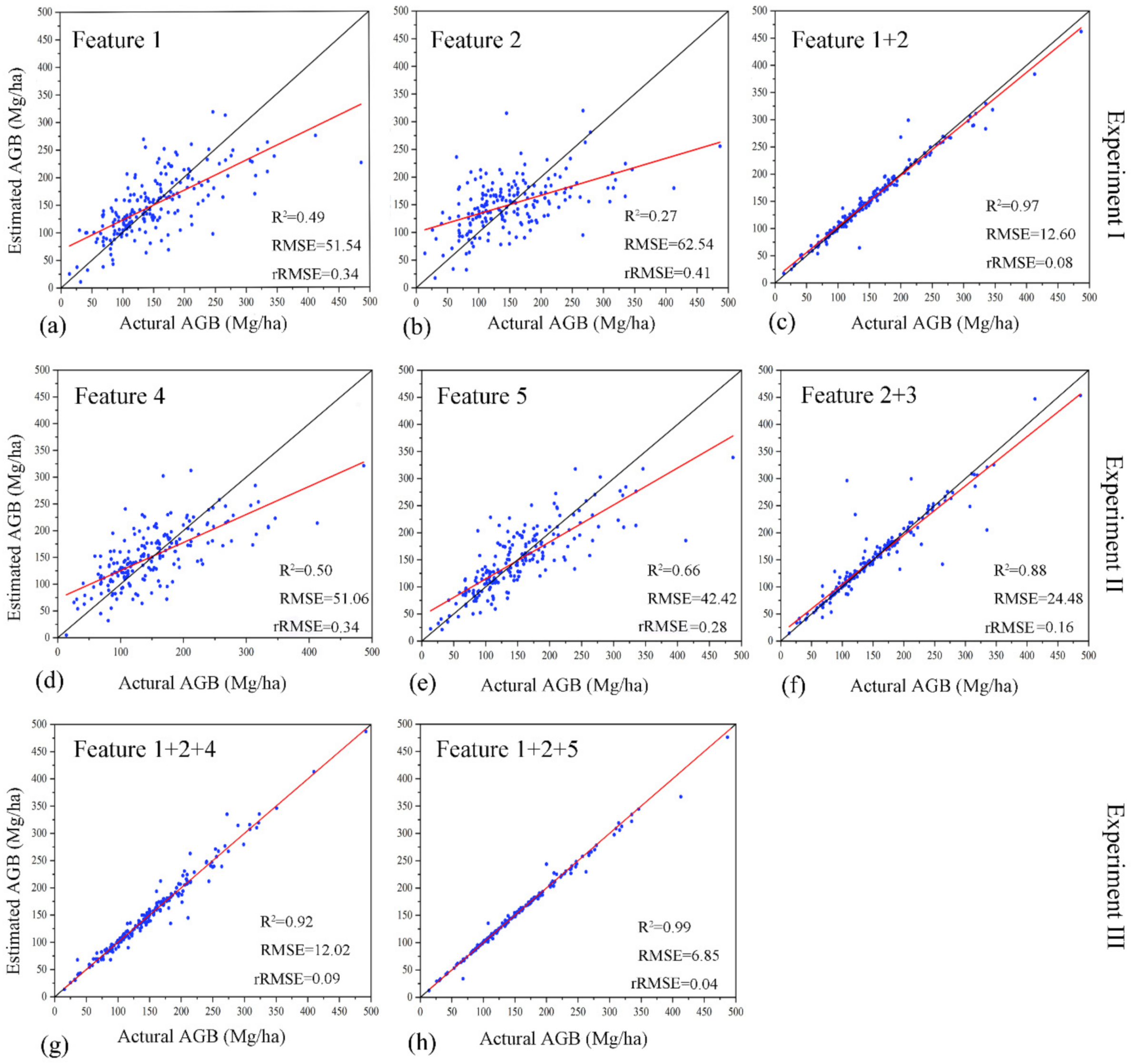
| CNN | 0.49 | 51.54 | 0.34 | 37.31 | 30.82 | 0.41 | |
| Optimal Landsat 8 features (Feature 2) | MLR | 0.17 | 66.36 | 0.47 | 58.08 | 44.31 | 1.05 |
| ELM | 0.12 | 71.64 | 0.48 | 59.73 | 41.40 | 1.21 | |
| BP | 0.13 | 68.58 | 0.49 | 57.19 | 42.76 | 1.04 | |
| RegT | 0.14 | 66.24 | 0.48 | 58.59 | 42.53 | 0.89 | |
| RF | 0.15 | 67.33 | 0.44 | 50.69 | 43.39 | 0.92 | |
| SVR | 0.07 | 70.31 | 0.46 | 51.65 | 47.28 | 1.14 | |
| KNN | 0.11 | 68.95 | 0.45 | 52.91 | 43.31 | 0.84 | |
| CNN | 0.27 | 62.54 | 0.41 | 47.16 | 43.08 | 0.72 | |
| Optimal ALS and Landsat 8 features (Feature 1 + 2) | MLR | 0.25 | 63.48 | 0.40 | 47.21 | 42.34 | 0.94 |
| ELM | 0.30 | 57.49 | 0.38 | 42.91 | 36.42 | 0.78 | |
| BP | 0.29 | 55.65 | 0.39 | 43.4 | 37.87 | 0.72 | |
| RegT | 0.24 | 60.86 | 0.45 | 55.07 | 39.18 | 0.87 | |
| RF | 0.28 | 61.91 | 0.41 | 45.36 | 39.28 | 0.91 | |
| SVR | 0.39 | 57.8 | 0.38 | 39.19 | 31.3 | 0.77 | |
| KNN | 0.22 | 65.37 | 0.43 | 48.6 | 34.69 | 1.07 | |
| CNN | 0.97 | 12.6 | 0.08 | 6.43 | 4.02 | 0.13 |
| Features | Algorithm | R2 | RMSE | rRMSE | MAE | MAPE | PM |
|---|---|---|---|---|---|---|---|
| All COLI1 (Feature 4) | MLR | 0.34 | 59.50 | 0.39 | 45.08 | 34.07 | 0.61 |
| ELM | 0.31 | 59.25 | 0.41 | 44.27 | 37.7 | 0.66 | |
| BP | 0.30 | 57.34 | 0.38 | 45.68 | 39.39 | 0.68 | |
| RegT | 0.28 | 62.62 | 0.43 | 50.22 | 45.45 | 0.72 | |
| RF | 0.32 | 60.14 | 0.40 | 43.27 | 35.55 | 0.62 | |
| SVR | 0.24 | 69.91 | 0.46 | 51.13 | 43.78 | 0.85 | |
| KNN | 0.26 | 62.58 | 0.41 | 46.3 | 38.39 | 0.69 | |
| CNN | 0.5 | 51.06 | 0.34 | 38.27 | 30.48 | 0.54 | |
| All COLI2 (Feature 5) | MLR | 0.22 | 61.49 | 0.48 | 50.12 | 39.34 | 0.72 |
| ELM | 0.25 | 64.35 | 0.47 | 51.07 | 40.81 | 0.75 | |
| BP | 0.30 | 62.14 | 0.47 | 50.39 | 38.24 | 0.78 | |
| RegT | 0.24 | 67.07 | 0.49 | 52.41 | 43.93 | 0.79 | |
| RF | 0.24 | 63.98 | 0.42 | 46.28 | 39.73 | 0.74 | |
| SVR | 0.26 | 67.69 | 0.45 | 49.05 | 38.71 | 0.78 | |
| KNN | 0.25 | 63.51 | 0.42 | 47.3 | 40.05 | 0.71 | |
| CNN | 0.66 | 42.42 | 0.28 | 29.71 | 22.16 | 0.45 | |
| Optimal Landsat 8 features + The best-performing ASL feature (Feature 2 + 3) | MLR | 0.33 | 60.14 | 0.40 | 44.45 | 40.76 | 0.70 |
| ELM | 0.29 | 64.26 | 0.43 | 48.39 | 42.59 | 0.69 | |
| BP | 0.30 | 63.8 | 0.41 | 50.11 | 44.01 | 0.70 | |
| RegT | 0.25 | 64.14 | 0.45 | 52.34 | 45.53 | 0.74 | |
| RF | 0.28 | 62.29 | 0.41 | 45.62 | 41.69 | 0.71 | |
| SVR | 0.29 | 62.25 | 0.41 | 42.00 | 40.21 | 0.82 | |
| KNN | 0.24 | 63.38 | 0.42 | 46.95 | 39.24 | 0.69 | |
| CNN | 0.88 | 24.48 | 0.16 | 10.19 | 7.23 | 0.24 |
| Features | Algorithm | R2 | RMSE | rRMSE | MAE | MAPE | PM |
|---|---|---|---|---|---|---|---|
| Optimal ALS + Landsat 8 features + All COLI1 (Feature 1 + 2 + 4) | MLR | 0.32 | 60.50 | 0.40 | 45.08 | 36.07 | 0.68 |
| ELM | 0.28 | 63.26 | 0.42 | 44.15 | 37.84 | 0.81 | |
| BP | 0.31 | 58.71 | 0.37 | 40.30 | 36.98 | 0.65 | |
| RegT | 0.28 | 62.07 | 0.42 | 42.29 | 38.51 | 0.79 | |
| RF | 0.31 | 60.32 | 0.41 | 43.41 | 39.26 | 0.73 | |
| SVR | 0.39 | 57.74 | 0.39 | 38.05 | 35.31 | 0.66 | |
| KNN | 0.29 | 61.11 | 0.44 | 42.87 | 36.47 | 0.69 | |
| CNN | 0.92 | 12.02 | 0.09 | 11.37 | 8.3 | 0.11 | |
| Optimal ALS + Landsat 8 features + All COLI2 (Feature 1 + 2 + 5) | MLR | 0.33 | 59.38 | 0.42 | 44.27 | 39.50 | 0.70 |
| ELM | 0.29 | 61.67 | 0.43 | 47.09 | 40.34 | 0.81 | |
| BP | 0.32 | 57.74 | 0.42 | 48.29 | 41.60 | 0.72 | |
| RegT | 0.33 | 65.59 | 0.42 | 49.26 | 42.17 | 0.83 | |
| RF | 0.31 | 60.61 | 0.40 | 44.69 | 31.08 | 0.69 | |
| SVR | 0.42 | 56.82 | 0.37 | 38.76 | 29.39 | 0.68 | |
| KNN | 0.32 | 59.83 | 0.39 | 44.34 | 37.3 | 0.64 | |
| CNN | 0.99 | 6.85 | 0.04 | 2.95 | 1.02 | 0.03 |
| Features | Algorithm | R2 | RMSE | rRMSE | MAE | MAPE | PM |
|---|---|---|---|---|---|---|---|
| Optimal ALS features (Feature 1) | SG(RF) | 0.20 | 65.38 | 0.43 | 50.66 | 42.35 | 1.03 |
| SG(SVR) | 0.24 | 63.98 | 0.42 | 45.75 | 41.03 | 0.92 | |
| SG(KNN) | 0.19 | 66.07 | 0.44 | 50.70 | 42.22 | 1.24 | |
| SG(CNN) | 0.61 | 45.42 | 0.30 | 31.59 | 24.28 | 0.37 | |
| Optimal Landsat 8 features (Feature 2) | SG(RF) | 0.44 | 54.24 | 0.36 | 40.20 | 32.47 | 0.57 |
| SG(SVR) | 0.45 | 54.36 | 0.36 | 38.85 | 34.59 | 0.65 | |
| SG(KNN) | 0.44 | 54.34 | 0.36 | 40.37 | 32.08 | 0.53 | |
| SG(CNN) | 0.76 | 35.28 | 0.23 | 24.29 | 18.17 | 0.26 | |
| Optimal ALS and Landsat 8 features (Feature 1 + 2) | SG(RF) | 0.93 | 18.04 | 0.12 | 8.78 | 6.30 | 0.17 |
| SG(SVR) | 0.97 | 12.13 | 0.08 | 5.70 | 4.70 | 0.14 | |
| SG(KNN) | 0.9 | 24.27 | 0.16 | 16.76 | 15.09 | 0.15 | |
| SG(CNN) | 0.97 | 10.95 | 0.07 | 6.58 | 5.06 | 0.03 |
| Features | Algorithm | R2 | RMSE | rRMSE | MAE | MAPE | PM |
|---|---|---|---|---|---|---|---|
| All COLI1 (Feature 4) | SG(RF) | 0.38 | 57.84 | 0.38 | 41.72 | 33.69 | 0.68 |
| SG(SVR) | 0.48 | 52.83 | 0.35 | 38.69 | 32.08 | 0.62 | |
| SG(KNN) | 0.36 | 58.5 | 0.39 | 43.04 | 34.36 | 0.71 | |
| SG(CNN) | 0.63 | 43.78 | 0.29 | 31.86 | 25.13 | 0.49 | |
| All COLI2 (Feature 5) | SG(RF) | 0.64 | 43.13 | 0.28 | 30.66 | 23.11 | 0.48 |
| SG(SVR) | 0.64 | 43.28 | 0.28 | 31.09 | 28.28 | 0.47 | |
| SG(KNN) | 0.60 | 45.85 | 0.30 | 32.74 | 27.00 | 0.51 | |
| SG(CNN) | 0.50 | 51.31 | 0.34 | 36.80 | 27.66 | 0.50 | |
| Optimal Landsat 8 features + The best-performing ALS feature (Feature 2 + 3) | SG(RF) | 0.86 | 26.94 | 0.18 | 14.22 | 10.66 | 0.24 |
| SG(SVR) | 0.88 | 24.61 | 0.16 | 10.13 | 10.25 | 0.29 | |
| SG(KNN) | 0.79 | 34.06 | 0.23 | 22.46 | 17.88 | 0.31 | |
| SG(CNN) | 0.86 | 26.45 | 0.17 | 14.76 | 10.35 | 0.2 |
| Features | Algorithm | R2 | RMSE | rRMSE | MAE | MAPE | PM |
|---|---|---|---|---|---|---|---|
| Optimal ALS + Landsat 8 features + All COLI1 (Feature 1 + 2 + 4) | SG(RF) | 0.95 | 15.35 | 0.11 | 12.44 | 9.34 | 0.14 |
| SG(SVR) | 0.71 | 58.84 | 0.38 | 24.02 | 15.76 | 0.49 | |
| SG(KNN) | 0.86 | 57.00 | 0.38 | 21.38 | 15.49 | 0.38 | |
| SG(CNN) | 0.97 | 12.35 | 0.08 | 2.02 | 1.07 | 0.03 | |
| Optimal ALS + Landsat 8 features + All COLI2 (Feature 1 + 2 + 5) | SG(RF) | 0.98 | 10.13 | 0.06 | 2.48 | 1.98 | 0.10 |
| SG(SVR) | 0.95 | 4.10 | 0.18 | 3.20 | 2.34 | 0.08 | |
| SG(KNN) | 0.96 | 15.76 | 0.10 | 9.04 | 8.28 | 0.17 | |
| SG(CNN) | 0.99 | 2.02 | 0.01 | 0.87 | 0.73 | 0.02 |
| Classic Algorithms | Runtime (s) | SG Algorithms | Runtime (s) |
|---|---|---|---|
| MLR | 1.2 | SG(RF) | 8168 |
| ELM | 45 | SG(SVR) | 7798 |
| BP | 38 | SG(KNN) | 7794 |
| RegT | 24 | SG(CNN) | 15170 |
| RF | 382 | ||
| SVR | 12 | ||
| KNN | 8 | ||
| CNN | 7384 |
Publisher’s Note: MDPI stays neutral with regard to jurisdictional claims in published maps and institutional affiliations. |
© 2021 by the authors. Licensee MDPI, Basel, Switzerland. This article is an open access article distributed under the terms and conditions of the Creative Commons Attribution (CC BY) license (https://creativecommons.org/licenses/by/4.0/).
Share and Cite
Du, C.; Fan, W.; Ma, Y.; Jin, H.-I.; Zhen, Z. The Effect of Synergistic Approaches of Features and Ensemble Learning Algorithms on Aboveground Biomass Estimation of Natural Secondary Forests Based on ALS and Landsat 8. Sensors 2021, 21, 5974. https://doi.org/10.3390/s21175974
Du C, Fan W, Ma Y, Jin H-I, Zhen Z. The Effect of Synergistic Approaches of Features and Ensemble Learning Algorithms on Aboveground Biomass Estimation of Natural Secondary Forests Based on ALS and Landsat 8. Sensors. 2021; 21(17):5974. https://doi.org/10.3390/s21175974
Chicago/Turabian StyleDu, Chunyu, Wenyi Fan, Ye Ma, Hung-Il Jin, and Zhen Zhen. 2021. "The Effect of Synergistic Approaches of Features and Ensemble Learning Algorithms on Aboveground Biomass Estimation of Natural Secondary Forests Based on ALS and Landsat 8" Sensors 21, no. 17: 5974. https://doi.org/10.3390/s21175974