
Complex Environment Path Planning for Unmanned Aerial Vehicles


Abstract
:1. Introduction
- In this paper, a BS-RRT algorithm is proposed to solve the global path planning problem. The algorithm converges quickly in the urban environment with narrow passages, and the algorithm has remarkable stability.
- To optimize the BS-RRT path further, a cyclic pruning algorithm is proposed to optimize the global programming path, and the effectiveness of the algorithm increases with the path’s tortuous degree.
- Local path adjustment depends on the prediction model. To improve the accuracy of the prediction model, this paper improves the calculation of the background value of the GM(1,1) model. At the same time, combined with the idea of metabolism, (the new method is presented to optimize the GM(1,1) model in this paper), which improves the prediction accuracy of the model greatly.
- This paper provides a feasible path planning scheme for UAV flight in a complex environment.
2. Related Work
3. Principles of Path Planning in Complex Environment
3.1. Global Path Planning
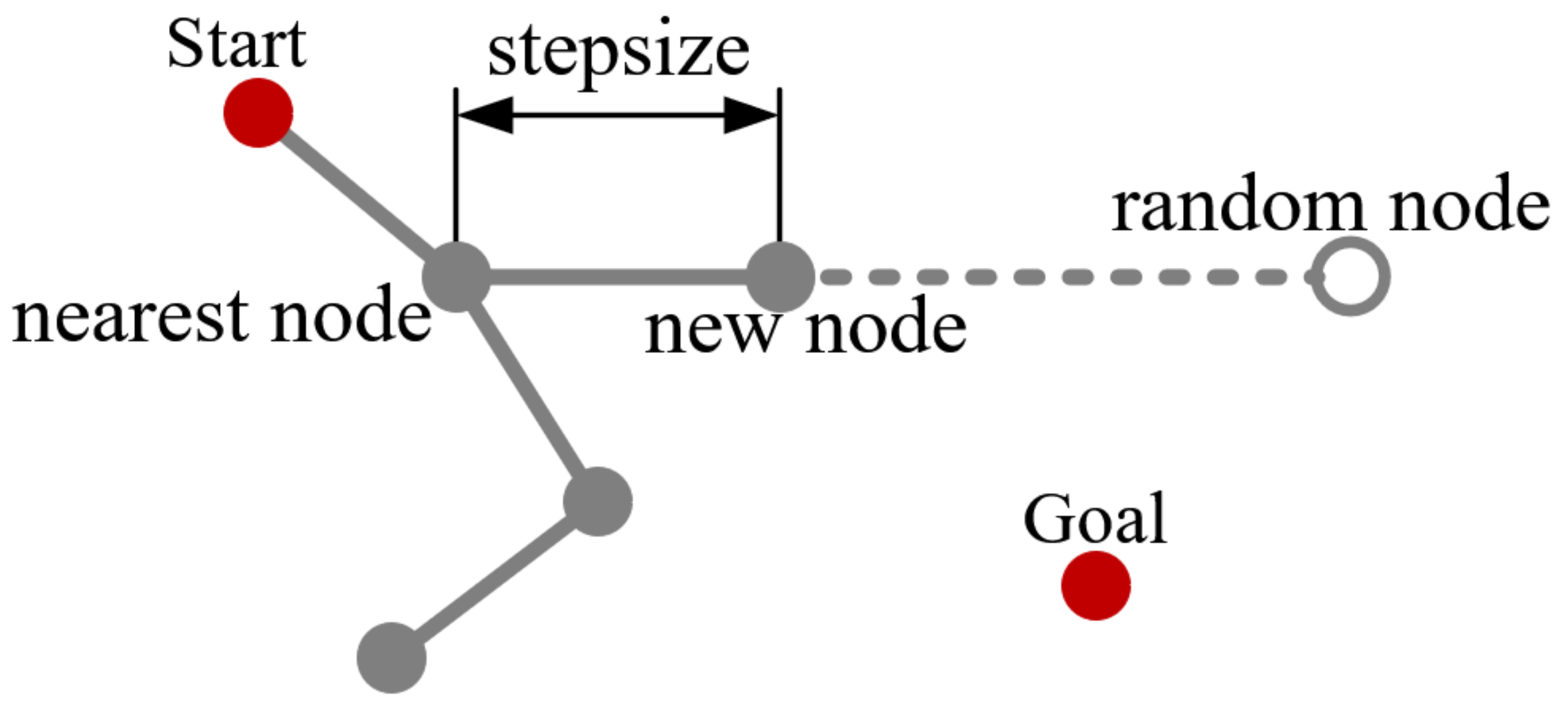
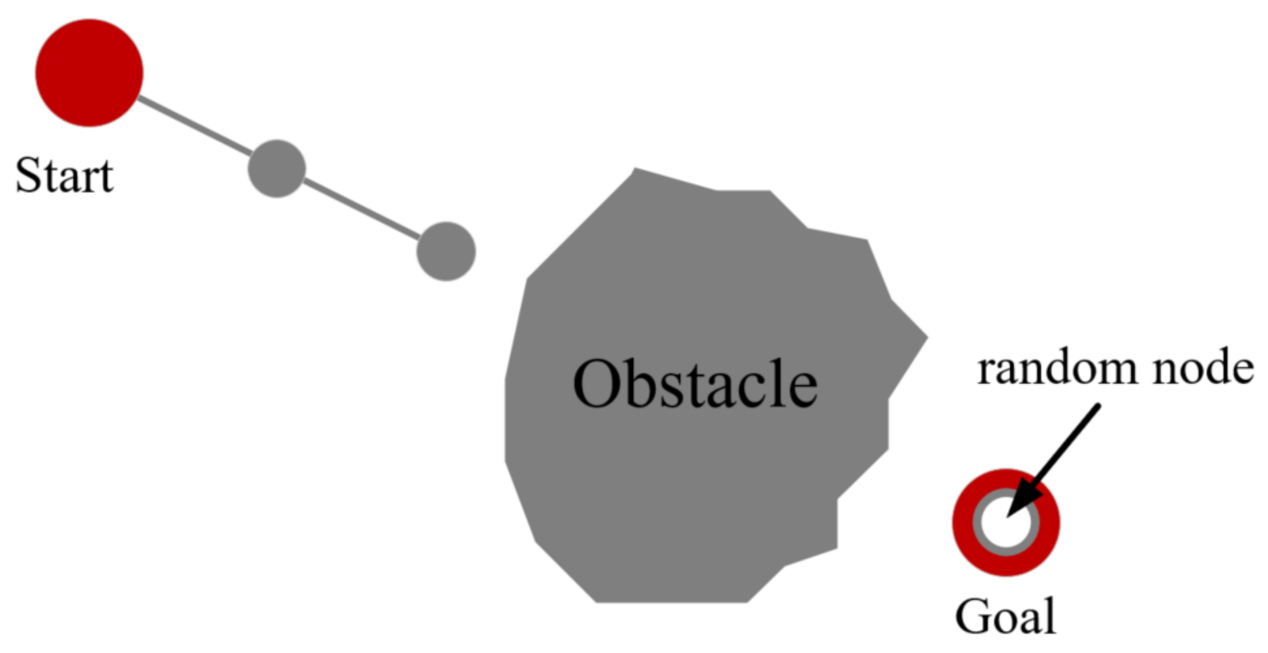
3.1.1. Principle of RRT
3.1.2. Principle of BS-RRT
- Greedy growthIn the initial phase, the sampling strategy is changed to speed up the tree expansion, and the sampling point for each sampling coincides with the goal point. In Figure 2, the BS-RRT continues to expand toward the goal point. The algorithm goes to the next stage when the BS-RRT fails to grow.
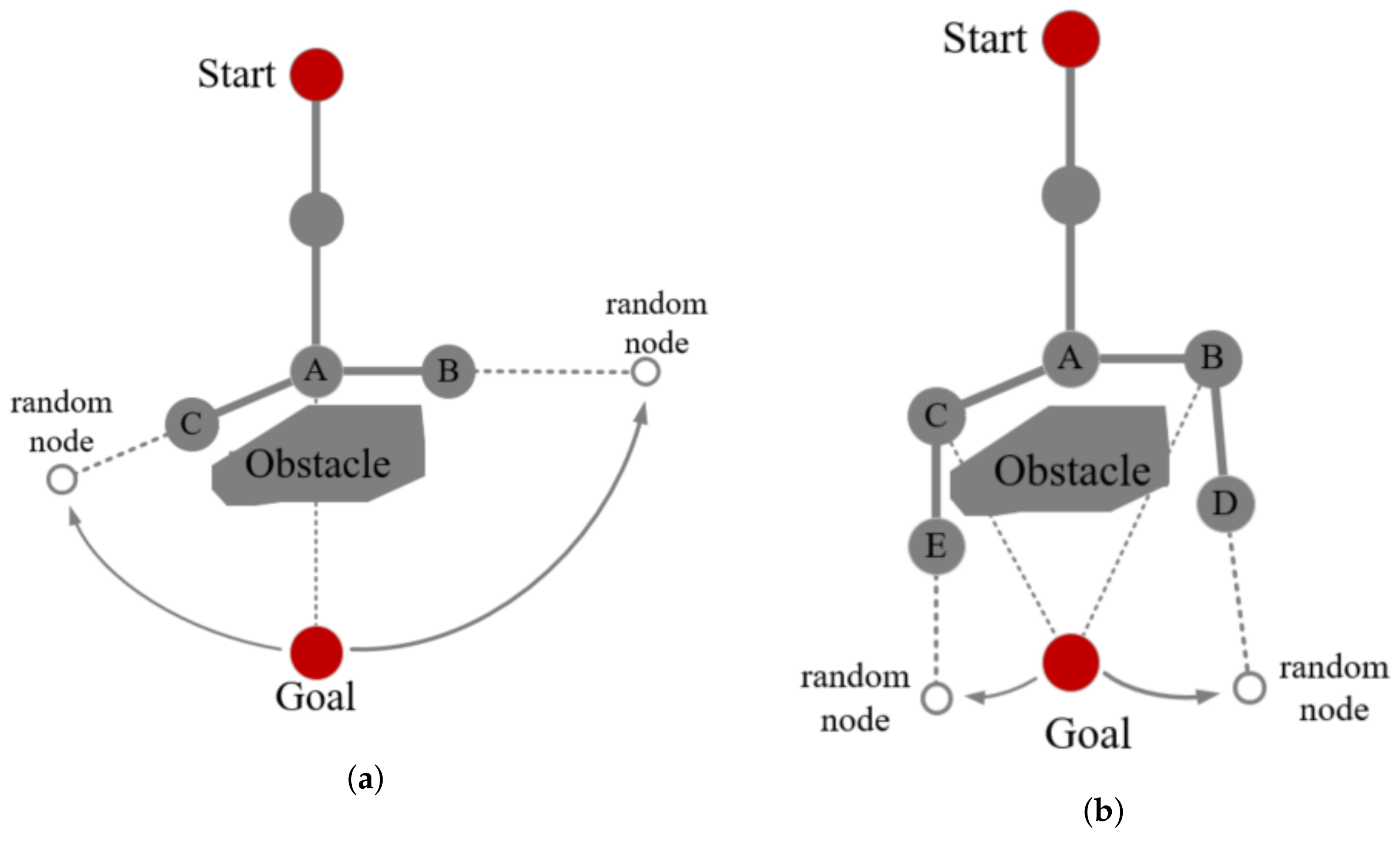
- Branch growthWhen the greedy growth stops, the BS-RRT tree will enter the branch growth stage to avoid obstacles. Point A in Figure 3a represents that point A failed to extend the next greedy point, and thus the point enters the branch, and point A is set as the root point of the branch. The line from the root point to the goal point divides the space into left and right regions. In the left region, the sampling point gradually moves away from the goal point in a clockwise trend each time, and the sampling stops until point C is expanded successfully. The sampling point in the right region gradually moves away from the goal point counterclockwise each sampling, the sampling stops until point B is extended successfully. In Figure 3b, points B and C cannot grow greedily because obstacles are observed in the direction from point B and C to the goal point. Hence, they continue to branch.The sampling point from point C to the direction of the goal point moves clockwise away from the goal point for each sampling until point E is expanded successfully. Similarly, the sampling point from point B points to the direction of the goal point moves counterclockwise away from the goal point each sampling until point D is expanded successfully. At this point, points E and D can grow greedily, and branch growth ends. Notably, in the branching stage, the length of the extension of all nodes is equal to the initial step size.Other branch nodes only expand one child node in addition to the original root point A. In the regions divided by root point A, the sampling point will only shift the sampling clockwise in the left region or counterclockwise sampling on the right, such as points C and E expand clockwise, meanwhile, points B and D expand counterclockwise. The branch growth in the corresponding region deviated to the direction of the goal point pointing to the leaf point to stop until the sampling point.
- Branch selectionWhen the branches stop growing, this indicates that BS-RRT has passed the barrier and enters the branch selection stage. If one branch fails to grow, then another branch will be selected directly. The overall BS-RRT algorithm will fail when both branches fail. The algorithm selects the branch with a short Euclidean distance from the goal point when the branches grow successfully. The selected leaf point of the branch as the starting point goes to the first step of greedy growth.
3.1.3. Cyclic Pruning Algorithm
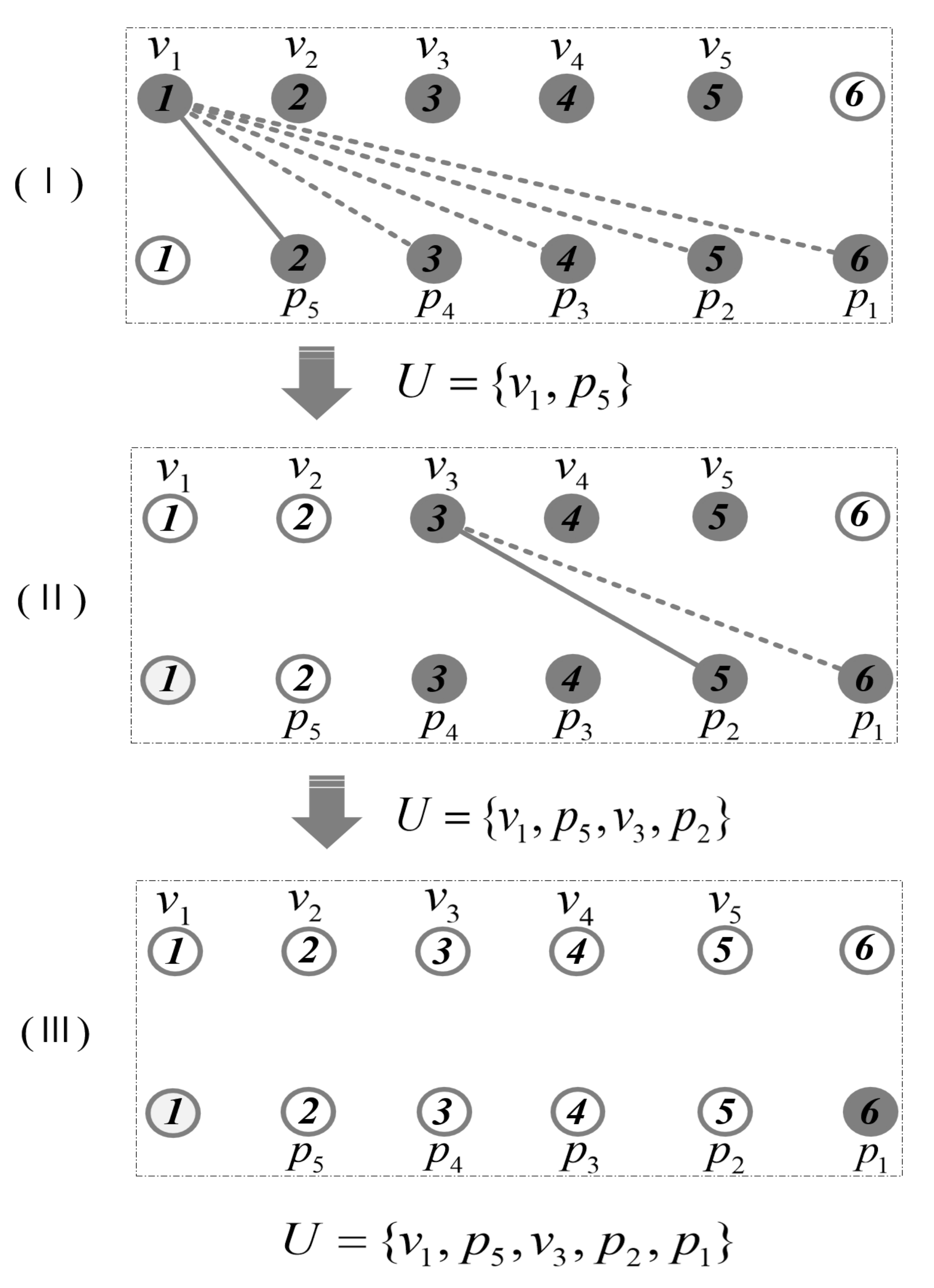
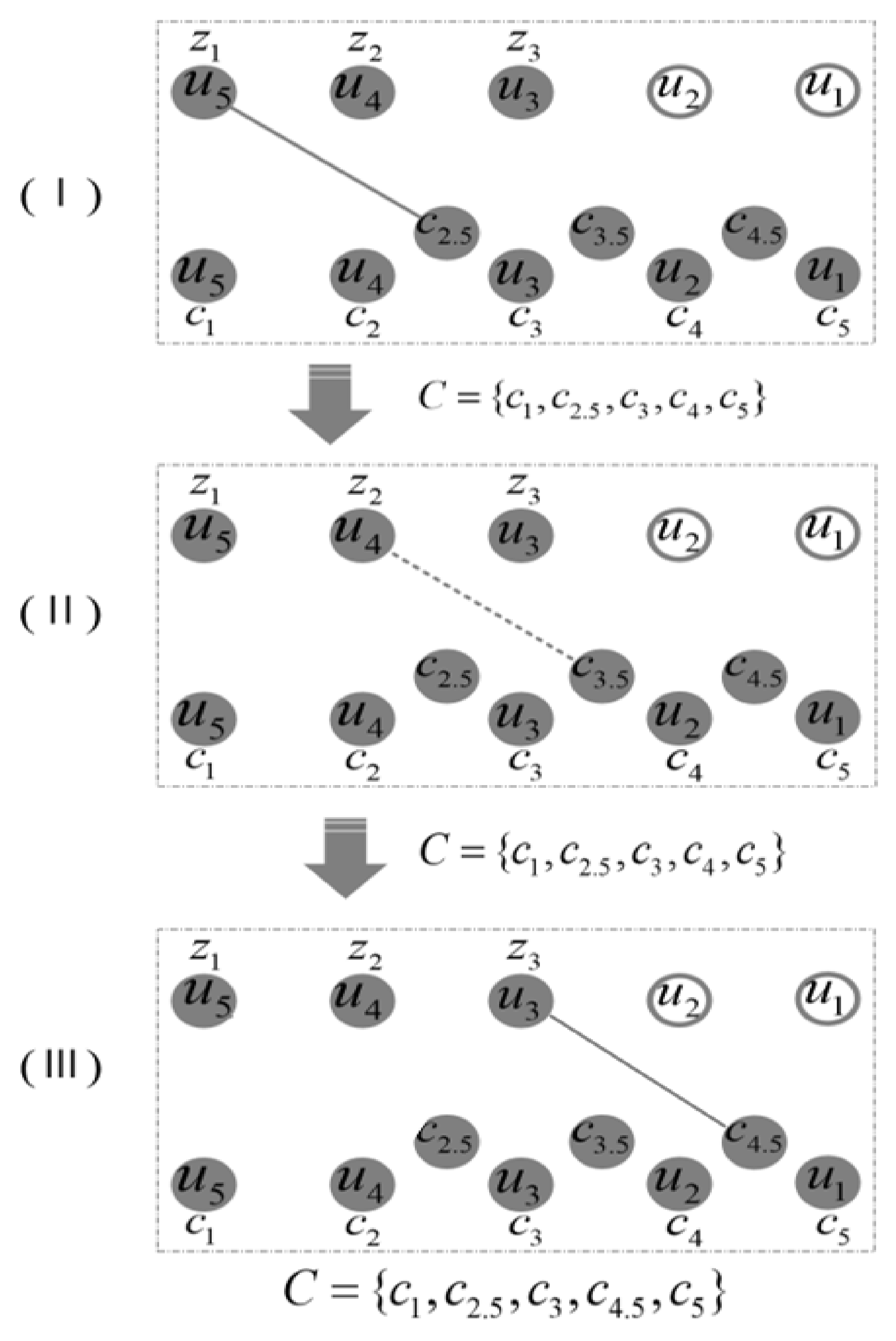
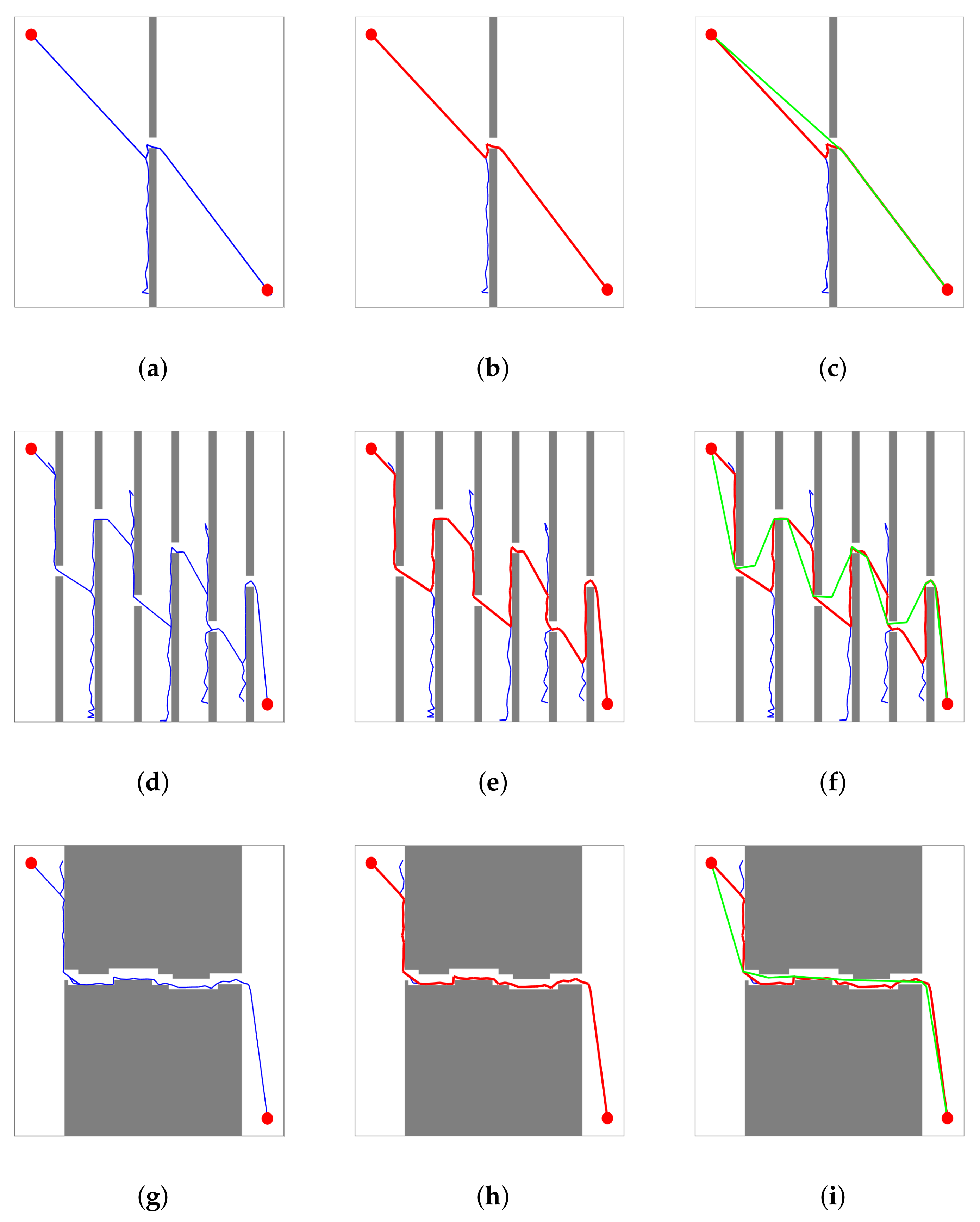
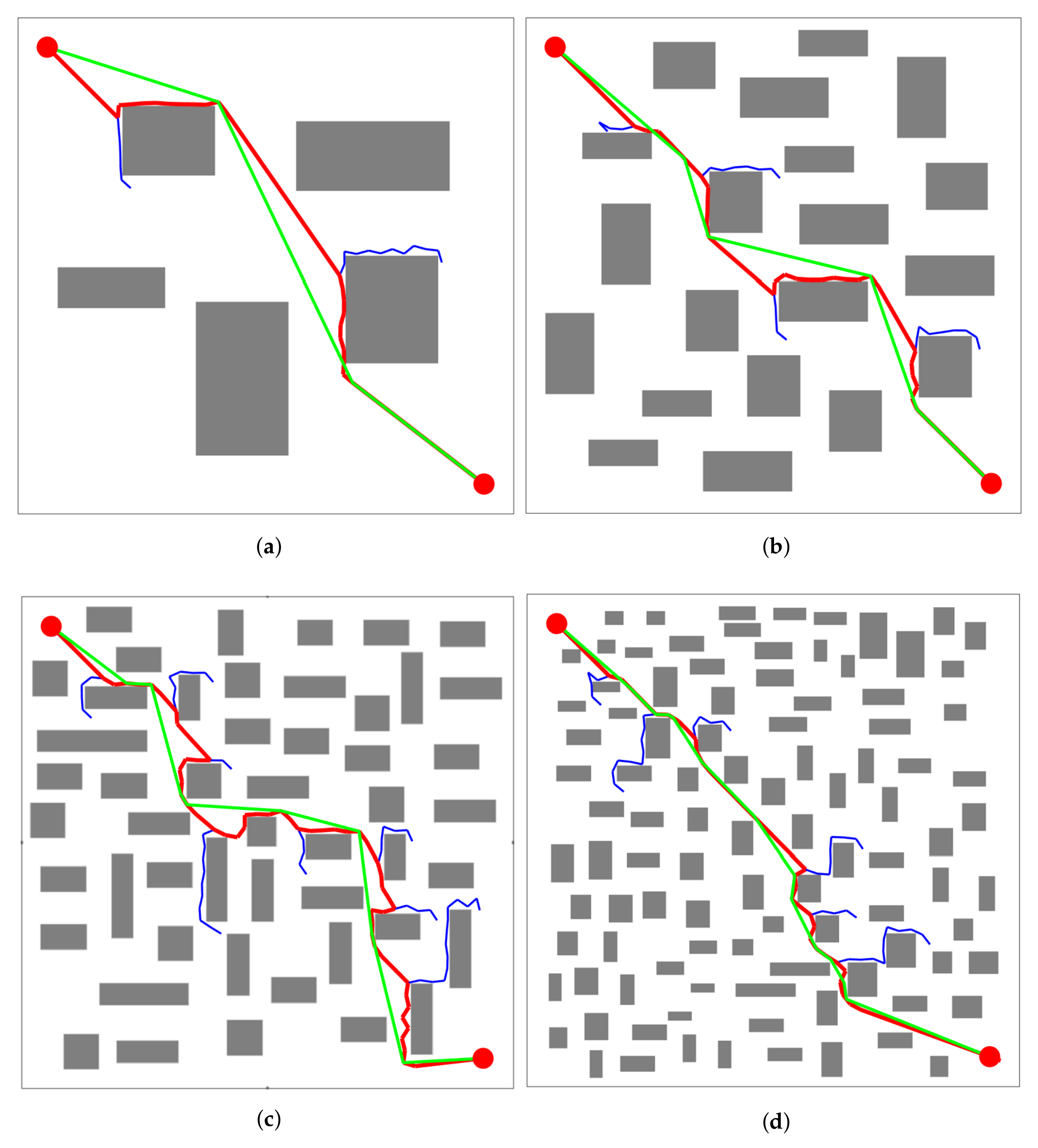
- The first pruningWe define the following set: set V = {, ,,…, }, set P = {, , ,…, }, and empty set U. Set V traverses every point in the path from the start point to the th point, set P traverses each point in the path from the end point nth to the third point in reverse, and the point in the set records the coordinate information of every point in the path. Based on the above definition, the point connecting to itself will be avoided.The first pruning of the path is performed as follows. First, we determine whether the point in the set V is connected to any point in set P. If the point and the point can be connected with no obstacle, then the points from to are deleted from the set V, the points from to are deleted from the set P as well. Meanwhile, the points and are added to set U.Repeat the above process until the set V is empty, point will be added to the set U if the point is not in the set U. The set U is the final result set after the first pruning. An example is shown in Figure 4 to describe the process of the first pruning in detail. There are seven points in the path generated by BS-RRT, where the hollow circles represent points that are not in sets V and P, dashed lines represent two points fail to connect due to the existence of obstacles, and solid lines represent two points can be connected directly. Thus, set V = {,,,,} and set P = {, , ,, } can be constructed. The first pruning operation is divided into three-steps in Figure 4.First, in determining whether the point in the set P can be connected to point , the initial value of j, j is set as 1. Figure 4I shows that point and can be connected directly. Then, points and are deleted from set V, point is deleted from set P, and point and are added to set U.Second, we determine whether the point in the set P can be connected to point in turn, and point and can be connected directly as shown in Figure 4II. Points , , and are deleted from set V, points , , and are deleted from set P, and points and are added to set U.Finally, the set V is empty in Figure 4III, the point will be added to the set U if is not in the set U. Thus, the set U = {,,,,}. All of points in the set V can be connected in turn, and the first pruning is finished.
- The second pruningAssume that there are m points in the set U after the first pruning, we define the following sets, set C = {,,,…, }, set Z = {,,,…, }. The points in set C represent the points in set U starting from to . The points in set Z represent the points in set U starting from point to point . The missing points and in set Z ensures that the connection of the last two points is not on the same line segment.The second pruning operation is performed as follows. Determining whether the first point in the set Z can be connected to the midpoint of the two points in the set C, that is, the midpoint of and connecting . If the connection is successful, then the midpoint of and —namely node —will replace the point in set C. Point will be determined in turn. After all the points in the point set Z are tested, the points in the set C forms the final path, and the cyclic pruning algorithm ends.An example is shown in Figure 5 to describe the process of the second pruning in detail. There are five points in the set U, the hollow circles represent points that are not in sets Z, dashed lines represent the failed connection between two points, and solid lines represent successful connections between two points. Set C = {,,,,} and set Z = {,,} are constructed accordingly.Similarly, the second pruning operation is divided into three steps in Figure 5. First, node is connected to node successfully, and then point is added to the set C to replace point . Second, point will not add to the set C because point failed to connect to point . Finally, point will replace point in the set C because point can be connected to node with no obstacle. The cyclic pruning algorithm ends and the set C is the final pruning result.
3.2. Trajectory Prediction of Dynamic Obstacles
3.2.1. Principle and Error Analysis of GM(1,1) Modeling
- Modeling of Grey Model GM(1,1)Let the original non-negative sequence data beFrom Equation (1), , and digital indicates that the initial data sequence. The is given as followswhereEquation (3) is first-order accumulated generation operating (1-AGO) series of . From Equation (3), we suppose that sequence meets the following first-order grad forecasting differential equationThe solution of Equation (4) with the initial condition is presented as followsThus, we obtained the following grey prediction equationHere, , is the predicted coordinate on the X axis. To obtain the prediction model of the raw data sequence, we need to determine the grey development coefficient a and the grey control parameter b in Equation (4). For this purpose, we performed the integral accumulation on both sides of Equation (4) for every contiguous interval, and then we can obtainLet the background value beConsequently, to estimate the values of a and b, we must use some methods to estimate the background value . We yield the estimated background value as followsThe method of solving parameters is expressed as
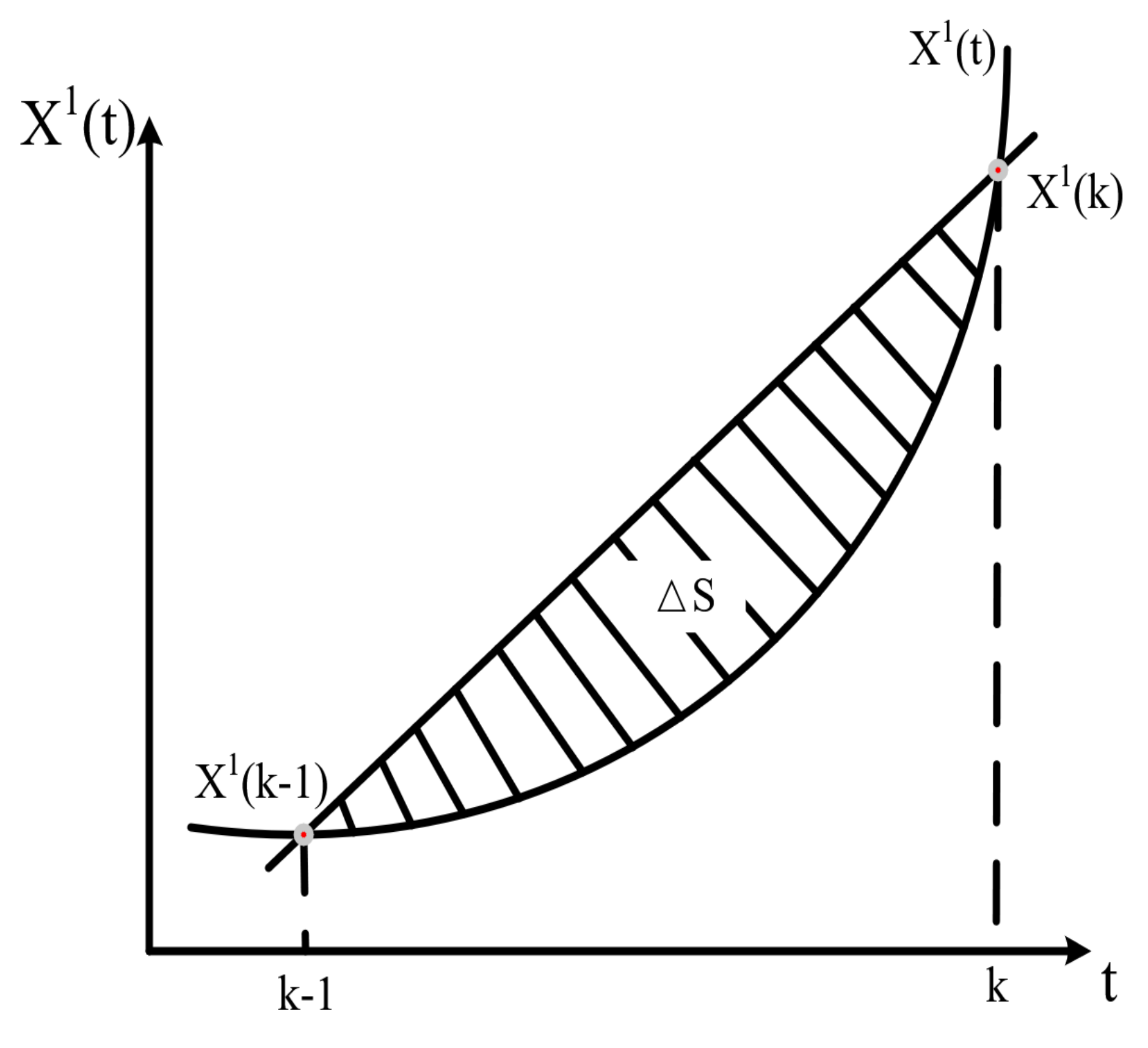
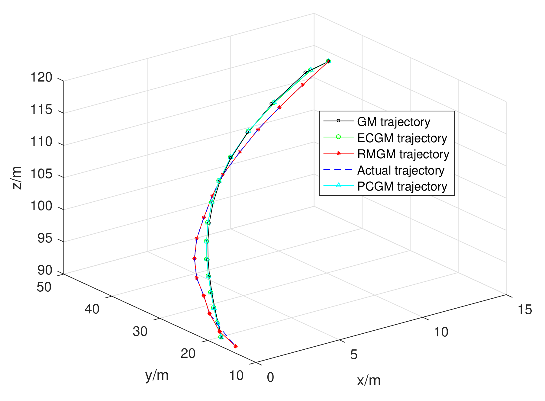
- Error analysisEquation (8) shows that the classical GM(1,1) model uses the average of adjacent values to estimate the background value . Its geometric meaning is that the trapezoidal area, which is based on the edge of exponential curve , has been replaced by the area of straight ladder. This method has significant error when the 1-AGO data sequence varies greatly. As shown in Figure 6, S is the error existing in the model.According to the error analysis results, the curve has fitting by first-order accumulation (1-AGO) dynamic sequence prediction model [43], and the trapezoidal area, which is based on the edge of the exponential curve , was recalculated by the Romberg numerical integration formula. Meanwhile, the optimized model was constructed by combining the idea of metabolism, named RMGM(1,1).
3.2.2. Principle of RMGM(1,1) Modeling
- 1-AGO dynamic sequence prediction model [43]Assume that Equations (1) and (2) meet the following law: If has the form of homogeneous exponential growth =, then the 1-AGO sequence is in the form of non-homogeneous exponential sequence (i.e., Equation (12)) and vice versa.The solving formula of each parameter is expressed as followsEquation (12) is called the 1-AGO dynamic sequence prediction model.
- Romberg quadrature formulaThe Romberg quadrature formula is also called the successively divided and semi-accelerated method. As an extrapolation algorithm, this formula improves the accuracy of the result of integration without increasing the amount of calculation. The Romberg quadrature formula has a more accurate integral approximate value by the weighted average of the approximate values of the trapezoidal formula.The initial parameter is set at , and the integral is calculated roughly asThe value of the next position is calculated asA recursive formula is used for the calculationIf the difference between and meets the predetermined accuracy , then the calculation stops. Otherwise, k goes up by 1, and then we proceed to Equation (17).The Romberg algorithm is expressed as the lower triangular matrix of Equation (18), and it can be extended infinitely downward and backward. The optimal approximate solution for a definite integral is , which is the lower right item calculated in Equation (19). The calculation of the Romberg quadrature formula recurs in Equations (17) and (18).
- Building a metabolic modelIn the traditional modeling process, the prediction accuracy of the model is reduced continuously as the system status changes by selecting a fixed length of the original data to build a model. Therefore, the higher prediction accuracy of the model should be ensured by updating the modeling data. This process of building a model is dynamic. The new data will be added to the modeling data sequence, and the oldest data in the modeling data will be deleted to reconstruct the model when a new data appears, the length of the modeling data of the construction of model remains unchanged. The optimal length of the modeling data will be discussed in the experiment.
- Construction of RMGM (1,1) modelThe RMGM(1,1) model reduces error by calculating the area of curve of the 1-AGO dynamic sequence model in each interval by using the Romberg quadrature formula.Step 1: Select a fixed-length raw data sequence and calculate 1-AGO sequence , .Step 2: Let , locate the interval , combine Equations (13)–(15) in this interval, and calculate the required parameters , A, and B of Equation (12) to obtain the formula .Step 3: Calculate r of the integral area of the interval in accordance with Equations (16)–(18). The ordinate value of the background value curve required by Equations (16)–(18) is given by Step 2, Let .Step 4: if , then proceed to Step 2, and let a and b increase by 1. The sequence of the background values is obtained until .Step 6: Newly generated data are added to the original data sequence , and the first old data are deleted at the same time. A new data sequence is generated by keeping the length unchanged, and then return to Step 1.
3.3. Local Path Adjustment
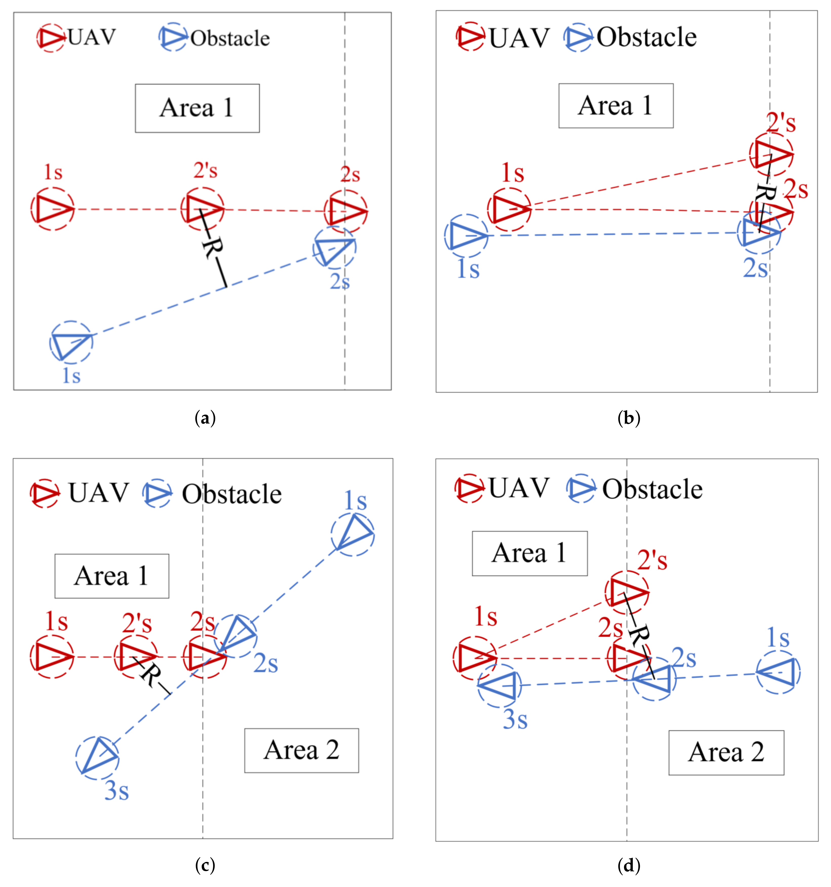
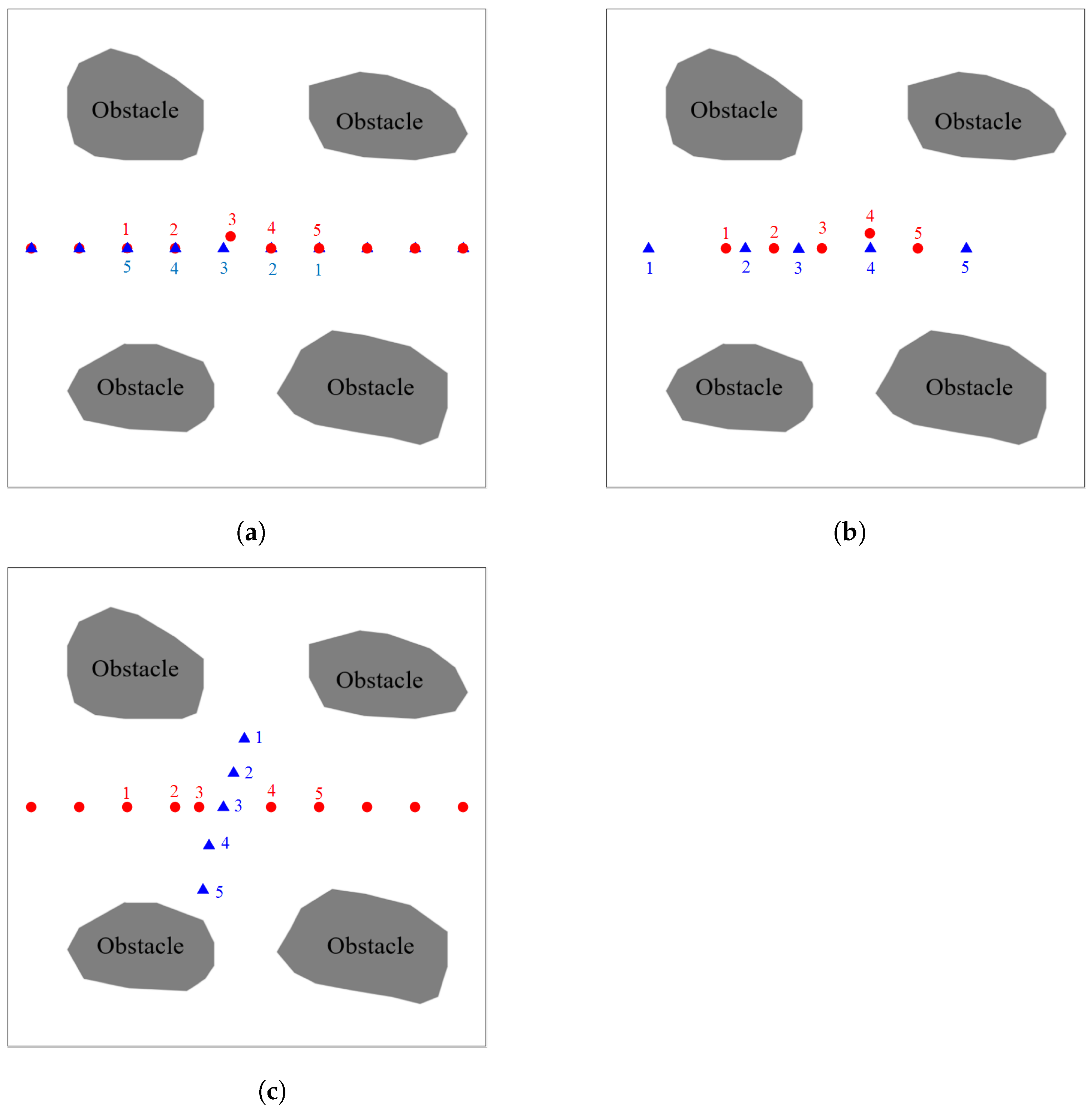
- In Figure 7a, the UAV verifies whether the adoption of a deceleration strategy is feasible, that is, the coordinate of 2’s is added to the original path instead of the coordinate of 2 s. R refers to the distance recorded between the UAV and the obstacle in every second. R should be greater than the sum of the radius of the envelopment circle of UAV and dynamic flight obstacle if no collision occurs. The path of the codirectional obstacle is not coincident with the path of the UAV and the R value is far greater than the sum of the radius of the envelope circle of UAV and the dynamic flight obstacle at 2’s. Therefore, the UAV will adopt this strategy wherein the position at 2’s replaces the position at 2 s.
- In Figure 7b, the path of the dynamic obstacle is coincident of the UAV. If the deceleration strategy is adopted, then the R value is less than the sum of the radius of the envelope circle of the UAV and the dynamic flight obstacle, and the collision will still occur. A decentralized strategy is adopted, the position at the 2 s is offset at the 2’s while keeping R greater than the sum of the radius of the envelope circle of the UAV and the dynamic flight obstacle. The UAV returns to the original path at 3 s after avoiding the dynamic obstacle. For the opposite dynamic obstacle, verifying whether the deceleration strategy is feasible first is necessary.
- In Figure 7c, if the deceleration strategy is adopted, then R is greater than the sum of the radius of the UAV and the dynamic flight obstacle envelope circle at the 2’s, and the position at the 2’s instead of the position at the 2 s add the path. Hence, obstacle avoidance is successful.
- In Figure 7d, the path of the UAV and dynamic obstacle are coincident, and R will be less than the sum of the radius of the enveloping circle of UAV and dynamic flight obstacle if the deceleration strategy is adopted. Thus, the decentralized strategy is carried out. The position at the 2’s is the offset position, thereby, making the R value greater than the sum of the radius of the envelopment circle of the UAV and the dynamic flight obstacle. The UAV returns to the original path at 3 s after successful obstacle avoidance.
4. Experiments and Discussions
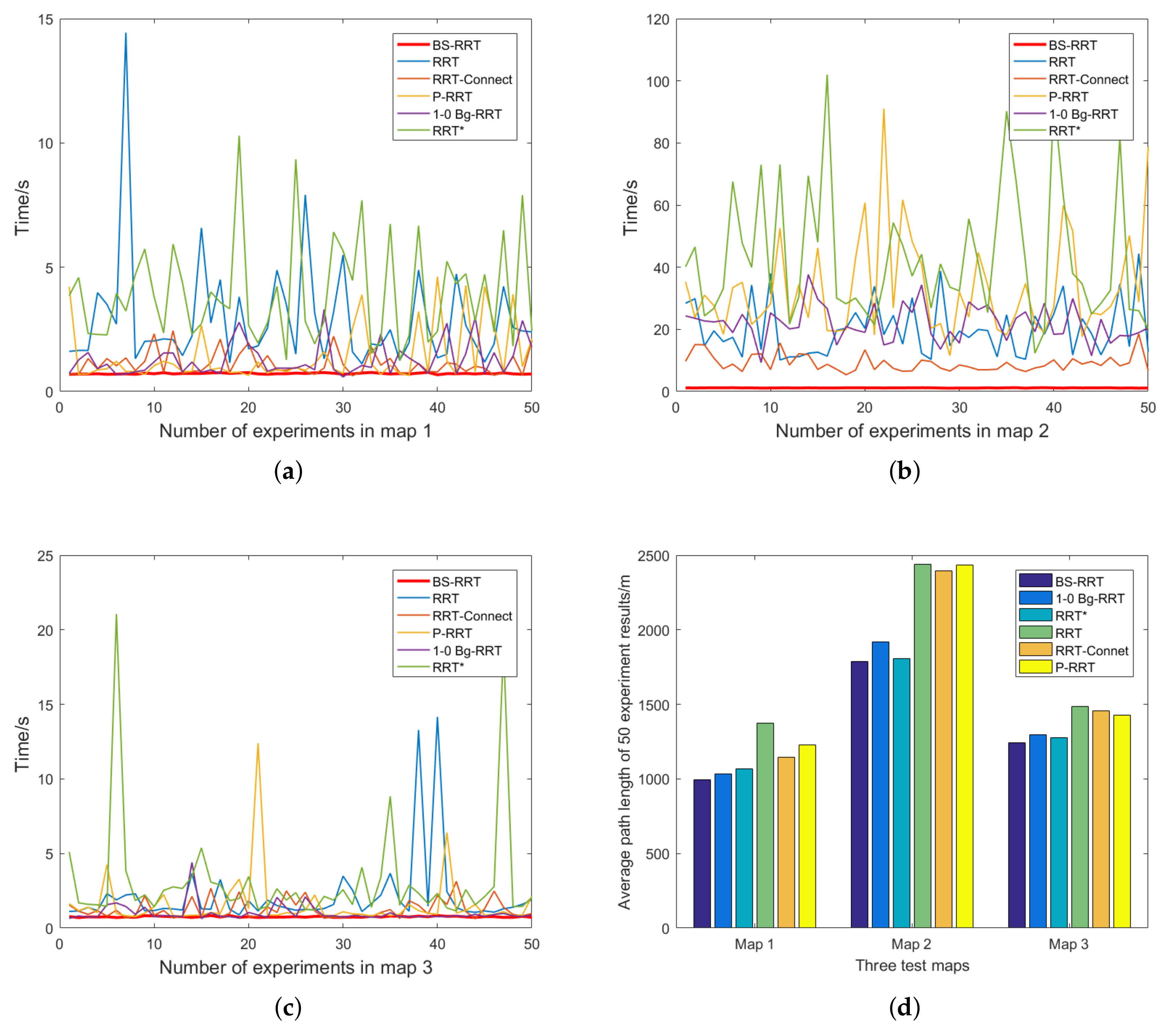
4.1. BS-RRT and the Circular Pruning Algorithm
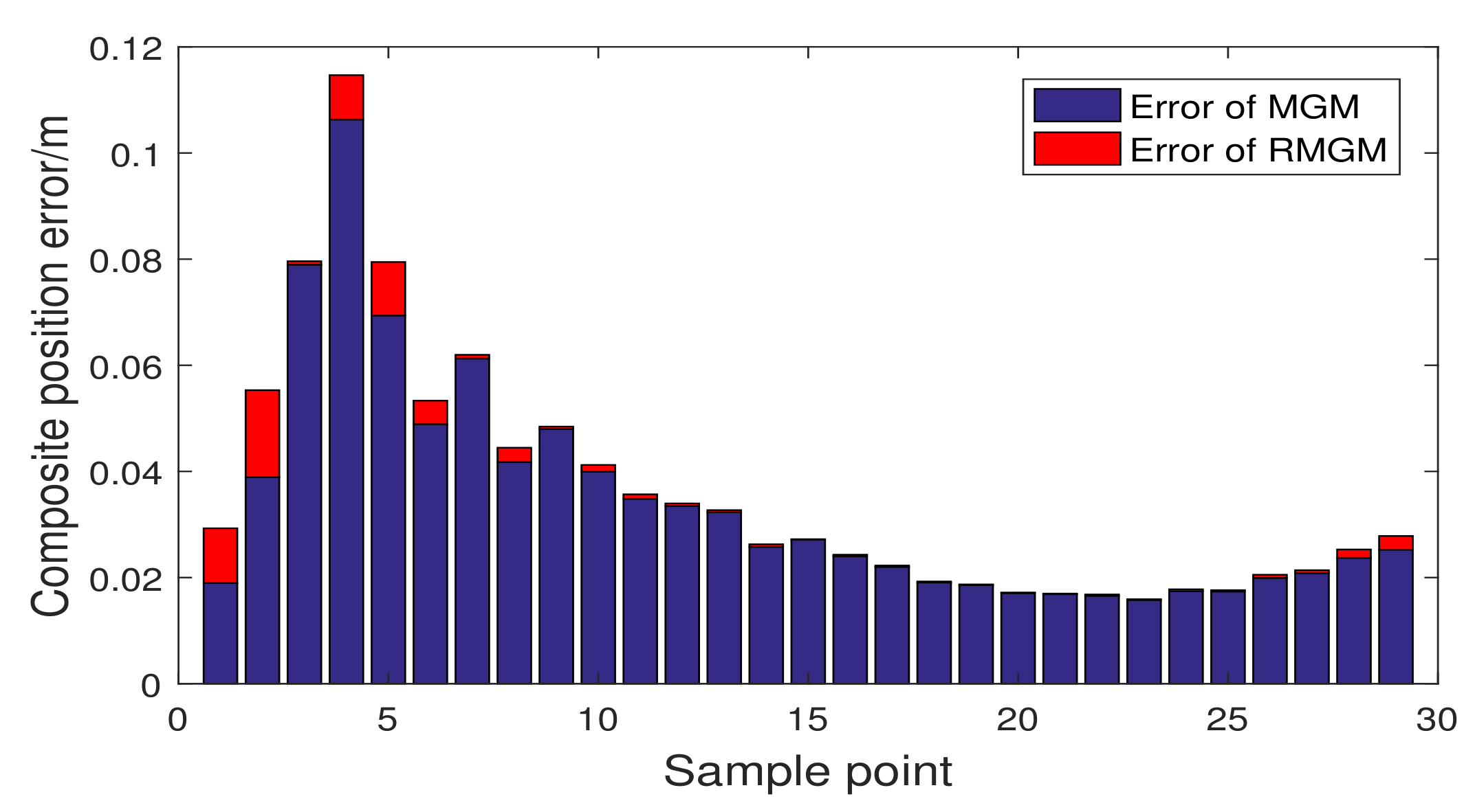
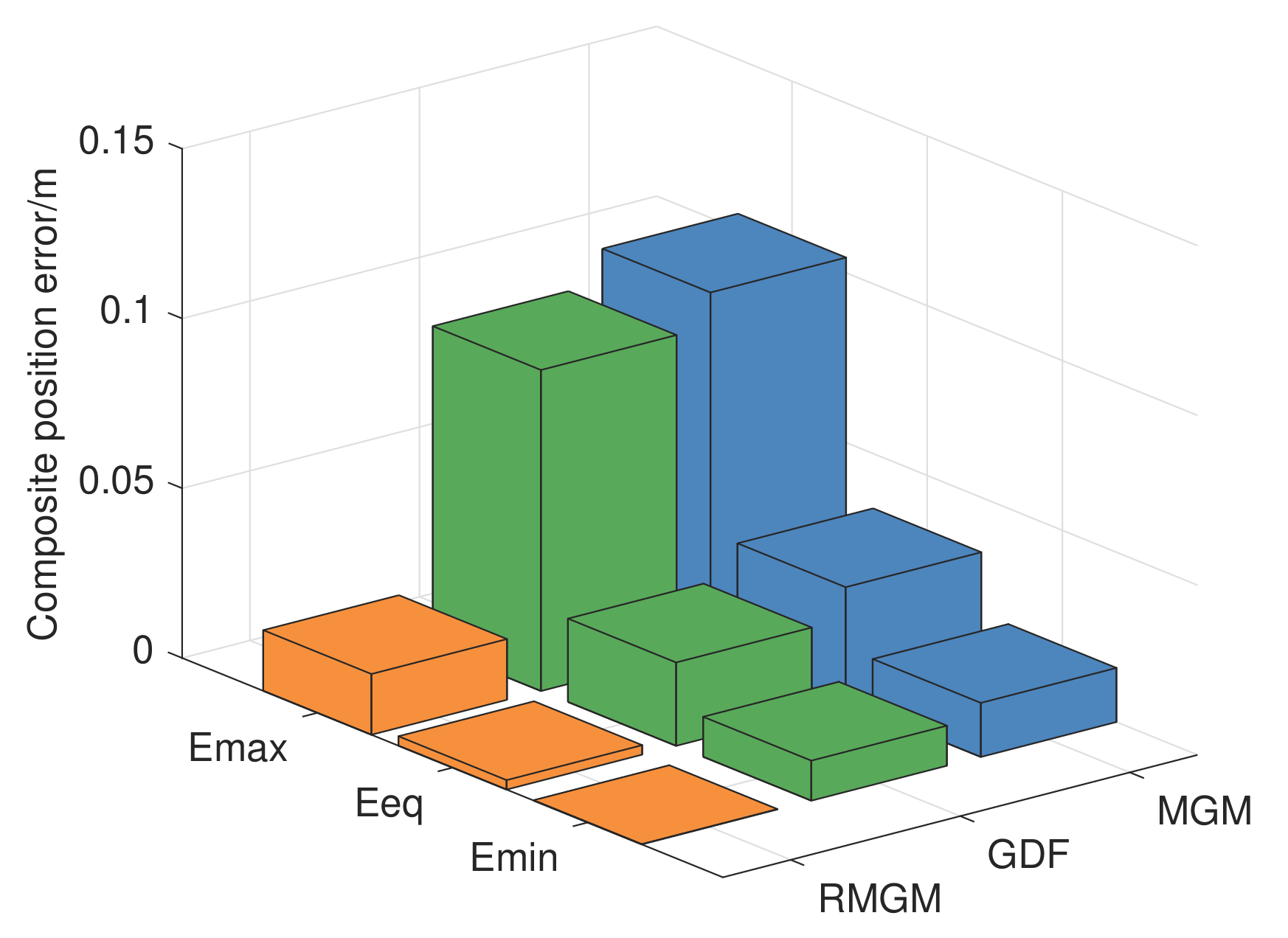
4.2. RMGM(1,1) Model Accuracy Comparison
4.3. Local Path Adjustment
5. Conclusions
Author Contributions
Funding
Institutional Review Board Statement
Informed Consent Statement
Data Availability Statement
Acknowledgments
Conflicts of Interest
References
- Garcin, M.; Desmazes, F.; Lerma, A.N.; Gouguet, L.; Météreau, V. Contribution of Lightweight Revolving Laser Scanner, HiRes UAV LiDARs and photogrammetry for characterization of coastal aeolian morphologies. J. Coast. Res. 2020, 95, 1094–1100. [Google Scholar] [CrossRef]
- Tripolitsiotis, A.; Prokas, N.; Kyritsis, S.; Dollas, A.; Papaefstathiou, I.; Partsinevelos, P. Dronesourcing: A modular, expandable multi-sensor UAV platform for combined, real-time environmental monitoring. Int. J. Remote Sens. 2017, 38, 2757–2770. [Google Scholar] [CrossRef]
- Wan, M.; Gu, G.; Qian, W.; Ren, K.; Maldague, X.; Chen, Q. Unmanned aerial vehicle video-based target tracking algorithm using sparse representation. IEEE Internet Things J. 2019, 6, 9689–9706. [Google Scholar] [CrossRef]
- Zheng, Y.; Du, Y.; Sheng, W.; Ling, H. Collaborative human-UAV search and rescue for missing tourists in nature reserves. INFORMS J. Appl. Anal. 2019, 49, 371–383. [Google Scholar] [CrossRef]
- Hart, P.E.; Nilsson, N.J.; Raphael, B. A formal basis for the heuristic determination of minimum cost paths. IEEE Trans. Syst. Sci. Cybern. 1968, 4, 100–107. [Google Scholar] [CrossRef]
- Stentz, A. The focussed D* algorithm for real-time replanning. In Proceedings of the 14th International Joint Conference on Artificial Intelligence, Montreal, QC, Canada, 20–25 August 1995; Volume 2, pp. 1652–1659. [Google Scholar]
- Koenig, S.; Likhachev, M. Fast replanning for navigation in unknown terrain. IEEE Trans. Robot. 2005, 21, 354–363. [Google Scholar] [CrossRef]
- Khatib, O. Real-time obstacle avoidance for manipulators and mobile robots. In Autonomous Robot Vehicles; Springer: Berlin/Heidelberg, Germany, 1986; pp. 396–404. [Google Scholar]
- Liu, A.; Jiang, J. Solving path planning problem based on logistic beetle algorithm search-pigeon-inspired optimisation algorithm. Electron. Lett. 2020, 56, 1105–1108. [Google Scholar] [CrossRef]
- Ok, S.H.; Seo, W.J.; Ahn, J.H.; Kang, S.; Moon, B. An ant colony optimization approach for the preference-based shortest path search. J. Chin. Inst. Eng. Trans. Chin. Inst. Eng. Ser. A 2011, 34, 181–196. [Google Scholar] [CrossRef]
- Kurdi, M.M.; Dadykin, A.K.; Elzein, I.; Ahmad, I.S. Proposed system of artificial Neural Network for positioning and navigation of UAV-UGV. In Proceedings of the 2018 Electric Electronics, Computer Science, Biomedical Engineerings’ Meeting (EBBT), Istanbul, Turkey, 18–19 April 2018; pp. 1–6. [Google Scholar]
- Zhang, Y.; Zhang, Y.; Liu, Z.; Yu, Z.; Qu, Y. Line-of-Sight Path Following Control on UAV with Sideslip Estimation and Compensation. In Proceedings of the 2018 37th Chinese Control Conference, Wuhan, China, 25–27 July 2018; pp. 4711–4716. [Google Scholar]
- LaValle, S.M. Rapidly-exploring random trees: A new tool for path planning. Comput. Sci. Dept. Oct. 1998, 98. Available online: https://www.cs.csustan.edu/~xliang/Courses/CS4710-21S/Papers/06%20RRT.pdf (accessed on 31 July 2021).
- Liu, J.; Shi, G.; Zhu, K. Online Multiple Outputs Least-Squares Support Vector Regression Model of Ship Trajectory Prediction Based on Automatic Information System Data and Selection Mechanism. IEEE Access 2020, 8, 154727–154745. [Google Scholar] [CrossRef]
- Chiou, J.; Yang, Y.; Chen, Y. Multivariate functional linear regression and prediction. J. Multivar. Anal. 2016, 146, 301–312. [Google Scholar] [CrossRef]
- Sun, S.; Chen, J.; Sun, J. Traffic congestion prediction based on GPS trajectory data. Int. J. Distrib. Sens. Netw. 2019, 15, 1550147719847440. [Google Scholar] [CrossRef]
- Qian, L.P.; Feng, A.; Yu, N.; Xu, W.; Wu, Y. Vehicular Networking-Enabled Vehicle State Prediction via Two-Level Quantized Adaptive Kalman Filtering. IEEE Internet Things J. 2020, 7, 7181–7193. [Google Scholar] [CrossRef]
- Wang, H.; Yang, Z.; Shi, Y. Next location prediction based on an adaboost-markov model of mobile users. Sensors 2019, 19, 1475. [Google Scholar] [CrossRef] [PubMed] [Green Version]
- Ding, J.; Liu, H.; Yang, L.T.; Yao, T.; Zuo, W. Multiuser Multivariate Multiorder Markov-Based Multimodal User Mobility Pattern Prediction. IEEE Internet Things J. 2019, 7, 4519–4531. [Google Scholar] [CrossRef]
- Ding, C.; Wang, W.; Wang, X.; Baumann, M. A Neural Network Model for Driver’s Lane-Changing Trajectory Prediction in Urban Traffic Flow. Math. Probl. Eng. 2013, 2013, 1–8. [Google Scholar] [CrossRef]
- Liu, M.; Shi, J. A cellular automata traffic flow model combined with a BP neural network based microscopic lane changing decision model. J. Intell. Transp. Syst. 2019, 23, 309–318. [Google Scholar] [CrossRef]
- Julong, D. Control problems of grey systems. Syst. Control Lett. 1982, 1, 288–294. [Google Scholar] [CrossRef]
- Zeng, B.; Duan, H.; Bai, Y.; Meng, W. Forecasting the output of shale gas in China using an unbiased grey model and weakening buffer operator. Energy 2018, 151, 238–249. [Google Scholar] [CrossRef]
- Ma, X.; Mei, X.; Wu, W.; Wu, X.; Zeng, B. A novel fractional time delayed grey model with Grey Wolf Optimizer and its applications in forecasting the natural gas and coal consumption in Chongqing China. Energy 2019, 178, 487–507. [Google Scholar] [CrossRef]
- Wu, W.; Ma, X.; Zhang, Y.; Wang, Y.; Wu, X. Analysis of novel FAGM (1, 1, t α) model to forecast health expenditure of China. Grey Syst. 2019, 9, 232–250. [Google Scholar] [CrossRef]
- Yershova, A.; Jaillet, L.; Siméon, T.; LaValle, S.M. Dynamic-domain RRTs: Efficient exploration by controlling the sampling domain. In Proceedings of the 2005 IEEE International Conference on Robotics and Automation, Barcelona, Spain, 18–22 April 2005; pp. 3856–3861. [Google Scholar]
- Jaillet, L.; Yershova, A.; La Valle, S.M.; Siméon, T. Adaptive tuning of the sampling domain for dynamic-domain RRTs. In Proceedings of the 2005 IEEE/RSJ International Conference on Intelligent Robots and Systems, Edmonton, AB, Canada, 2–6 August 2005; pp. 2851–2856. [Google Scholar]
- Gan, Y.; Zhang, B.; Ke, C.; Zhu, X.; He, W.; Ihara, T. Research on Robot Motion Planning Based on RRT Algorithm with Nonholonomic Constraints. Neural Process. Lett. 2021, 53, 3011–3029. [Google Scholar] [CrossRef]
- Dalibard, S.; Laumond, J.P. Control of probabilistic diffusion in motion planning. In Algorithmic Foundation of Robotics VIII; Springer: Berlin/Heidelberg, Germany, 2009; pp. 467–481. [Google Scholar]
- Burns, B.; Brock, O. Single-query motion planning with utility-guided random trees. In Proceedings of the 2007 IEEE International Conference on Robotics and Automation, Roma, Italy, 10–14 April 2007; pp. 3307–3312. [Google Scholar]
- Kuffner, J.J.; LaValle, S.M. RRT-connect: An efficient approach to single-query path planning. In Proceedings of the 2000 ICRA. Millennium Conference. IEEE International Conference on Robotics and Automation. Symposia Proceedings, San Francisco, CA, USA, 24–28 April 2000; Volume 2, pp. 995–1001. [Google Scholar]
- Li, T.; Shie, Y. An incremental learning approach to motion planning with roadmap management. In Proceedings of the 2002 IEEE International Conference on Robotics and Automation, Washington, DC, USA, 11–15 May 2002; Volume 4, pp. 3411–3416. [Google Scholar]
- Otte, M.; Correll, N. C-FOREST: Parallel shortest path planning with superlinear speedup. IEEE Trans. Robot. 2013, 29, 798–806. [Google Scholar] [CrossRef]
- Strandberg, M. Augmenting RRT-planners with local trees. In Proceedings of the IEEE International Conference on Robotics and Automation, New Orleans, LA, USA, 26 April–1 May 2004; Volume 4, pp. 3258–3262. [Google Scholar]
- Tan, G. The structure method and application of background value in grey system GM(1, 1) model (I). Syst. Eng. Theory Pract. 2000, 20, 98–103. [Google Scholar]
- Guanjun, T. The Structure Method and Application of Background Value in Grey System GM(1, 1) model (II). Syst. Eng. Theory Pract. 2000, 5, 125–132. [Google Scholar]
- Sun, J.; Li, H.; Zeng, B.; Zhao, X.; Wang, C. Parameter Optimization on the Three-Parameter Whitenization Grey Model and Its Application in Simulation and Prediction of Gross Enrollment Rate of Higher Education in China. Complexity 2020, 2020, 1–10. [Google Scholar]
- Yuhong, W.; Jie, L. Improvement and application of GM(1, 1) model based on multivariable dynamic optimization. J. Syst. Eng. Electron. 2020, 31, 593–601. [Google Scholar] [CrossRef]
- Cheng, M.; Shi, G. Improved methods for parameter estimation of gray model GM(1, 1) based on new background value optimization and model application. Commun. Stat. Simul. Comput. 2019, 1–23. [Google Scholar] [CrossRef]
- Zhu, Y.; Jian, Z.; Du, Y.; Chen, W.; Fang, J. A New GM(1, 1) Model Based on Cubic Monotonicity-Preserving Interpolation Spline. Symmetry 2019, 11, 420. [Google Scholar] [CrossRef] [Green Version]
- Li, K.; Liu, L.; Zhai, J.; Khoshgoftaar, T.M.; Li, T. The improved grey model based on particle swarm optimization algorithm for time series prediction. Eng. Appl. Artif. Intell. 2016, 55, 285–291. [Google Scholar] [CrossRef]
- Chen, Y. High-order polynomial interpolation based on the interpolation center’s neighborhood the amendment to the runge phenomenon. In Proceedings of the 2009 WRI World Congress on Software Engineering, Xiamen, China, 19–21 May 2009; Volume 2, pp. 345–348. [Google Scholar]
- Wang, Z.; Dang, Y.; Liu, S.; Zhou, J. The optimization of background value in GM(1, 1) model. J. Grey Syst. 2007, 10, 69–74. [Google Scholar] [CrossRef]
- Ju, Q.; Li, H.; Zhang, Y. Power management for kinetic energy harvesting IoT. IEEE Sens. J. 2018, 18, 4336–4345. [Google Scholar] [CrossRef]
- Ju, Q.; Zhang, Y. Predictive power management for internet of battery-less things. IEEE Trans. Power Electron. 2017, 33, 299–312. [Google Scholar] [CrossRef]
- Lin, Y.; Saripalli, S. Sampling-based path planning for UAV collision avoidance. IEEE Trans. Intell. Transp. Syst. 2017, 18, 3179–3192. [Google Scholar] [CrossRef]
- Wang, Q.; Zhang, Z.; Wang, Z.; Wang, Y.; Zhou, W. The trajectory prediction of spacecraft by grey method. Meas. Sci. Technol. 2016, 27, 085011. [Google Scholar] [CrossRef]
- Xia, X.; Chen, X.; Zhang, Y.; Wang, Z. Grey bootstrap method of evaluation of uncertainty in dynamic measurement. Measurement 2008, 41, 687–696. [Google Scholar] [CrossRef]
- Luo, Z.; Wang, Y.; Zhou, W.; Wang, Z. The grey relational approach for evaluating measurement uncertainty with poor information. Meas. Sci. Technol. 2015, 26, 125002. [Google Scholar] [CrossRef]


| Experiment | Parameters |
|---|---|
| Runtime environment | IntelCPU2.8G 16 GB memory computer using MATLAB-R2016B |
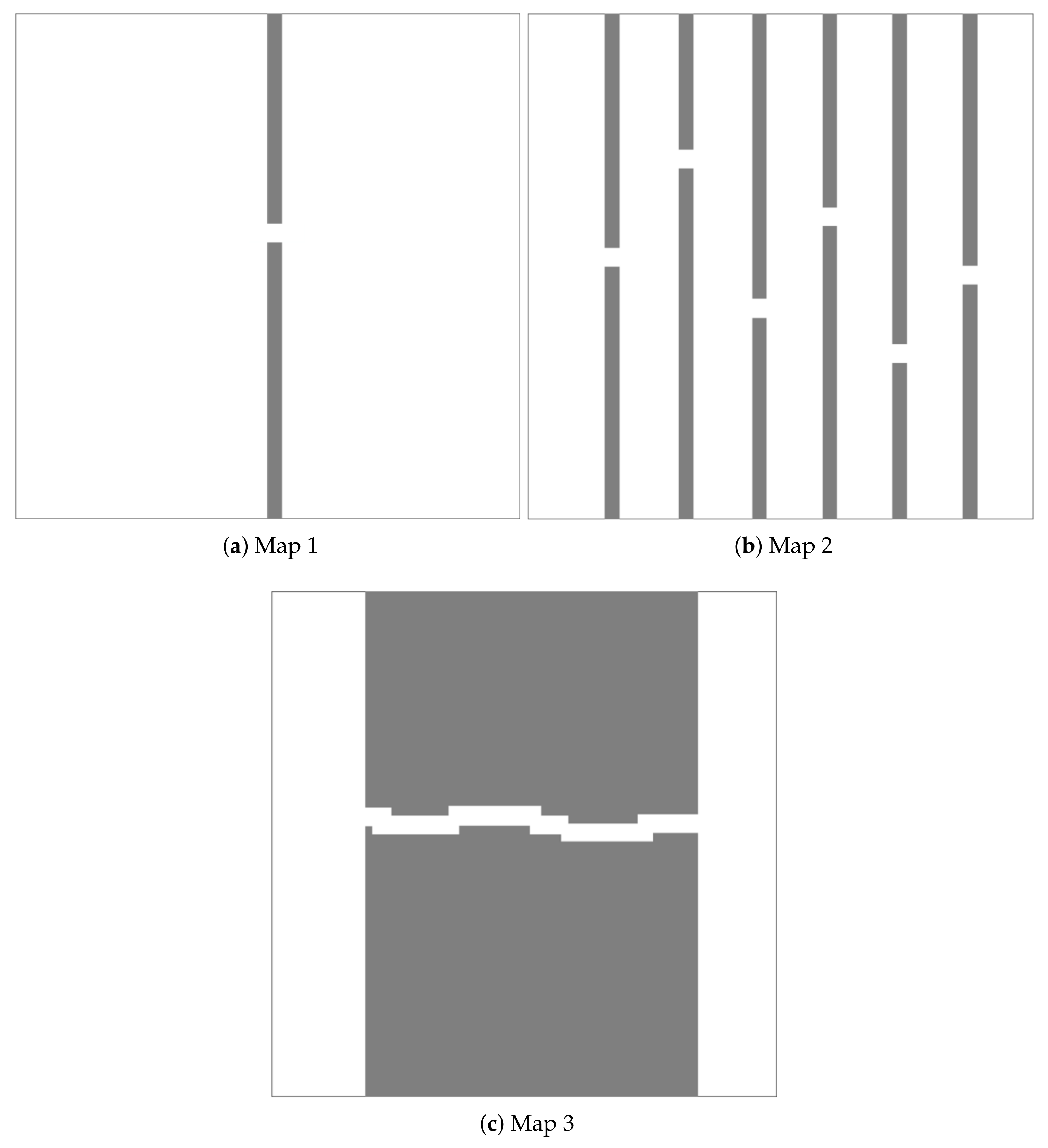
| Map size | 800 × 800 |
| Number of maps | 3 |
| Start point in the map | (50,50) |
| Goal point in the map | (750,750) |
| Narrow passage width | 30 |
| Envelope sphere radius of UA V and dynamic flight obstacle | 0.5 |
| Narrow passage width | 30 |
| Distance R | 2 |
| Figure | Before Pruning | After Pruning | Percentage Reduction |
|---|---|---|---|
| Figure 9c | 1054.345 | 995.238 | 5.606% |
| Figure 9f | 2369.049 | 1779.210 | 24.898% |
| Figure 9i | 1505.181 | 1248.134 | 17.077% |
| Map | Algorithm | Average Planning Time/s | Maximum Time Difference/s | Average Path Length |
|---|---|---|---|---|
| Map 1 | BS-RRT | 0.722 | 0.097 | 994.858 |
| RRT | 2.905 | 13.324 | 1374.577 | |
| RRT-Connect | 1.121 | 2.449 | 1146.323 | |
| P-RRT | 1.466 | 4.621 | 1225.728 | |
| 1-0 Bg-RRT | 1.304 | 2.628 | 1033.617 | |
| RRT | 3.951 | 9.050 | 1068.216 | |
| Map 2 | BS-RRT | 1.159 | 0.162 | 1787.360 |
| RRT | 20.020 | 34.189 | 2439.182 | |
| RRT-Connect | 9.152 | 18.563 | 2396.566 | |
| P-RRT | 33.216 | 91.061 | 2433.546 | |
| 1-0 Bg-RRT | 21.898 | 28.304 | 1920.761 | |
| RRT | 42.886 | 89.655 | 1807.956 | |
| Map 3 | BS-RRT | 0.757 | 0.136 | 1242.084 |
| RRT | 2.127 | 13.274 | 1486.449 | |
| RRT-Connect | 1.270 | 3.126 | 1457.493 | |
| P-RRT | 1.567 | 12.392 | 1429.350 | |
| 1-0 Bg-RRT | 1.008 | 3.768 | 1298.581 | |
| RRT | 3.115 | 19.911 | 1274.754 |
| Figure | Maximum Time Difference/s | Minimum Planning Time/s | Average Planning Time/s | Maximum Planning Time/s |
|---|---|---|---|---|
| Figure 12a | 0.1277 | 0.7388 | 0.8169 | 0.8665 |
| Figure 12b | 0.1367 | 0.7632 | 0.8556 | 0.8999 |
| Figure 12c | 0.1530 | 0.8429 | 0.9452 | 0.9959 |
| Figure 12d | 0.2754 | 0.8387 | 0.9456 | 1.1141 |
| Figure | Before Pruning | After Pruning | Percentage Reduction |
|---|---|---|---|
| Figure 12a | 1105.35 | 1046.38 | 5.33% |
| Figure 12b | 1168.98 | 1059.44 | 9.37% |
| Figure 12c | 1199.60 | 1062.18 | 11.46% |
| Figure 12d | 1228.31 | 1108.53 | 9.75% |
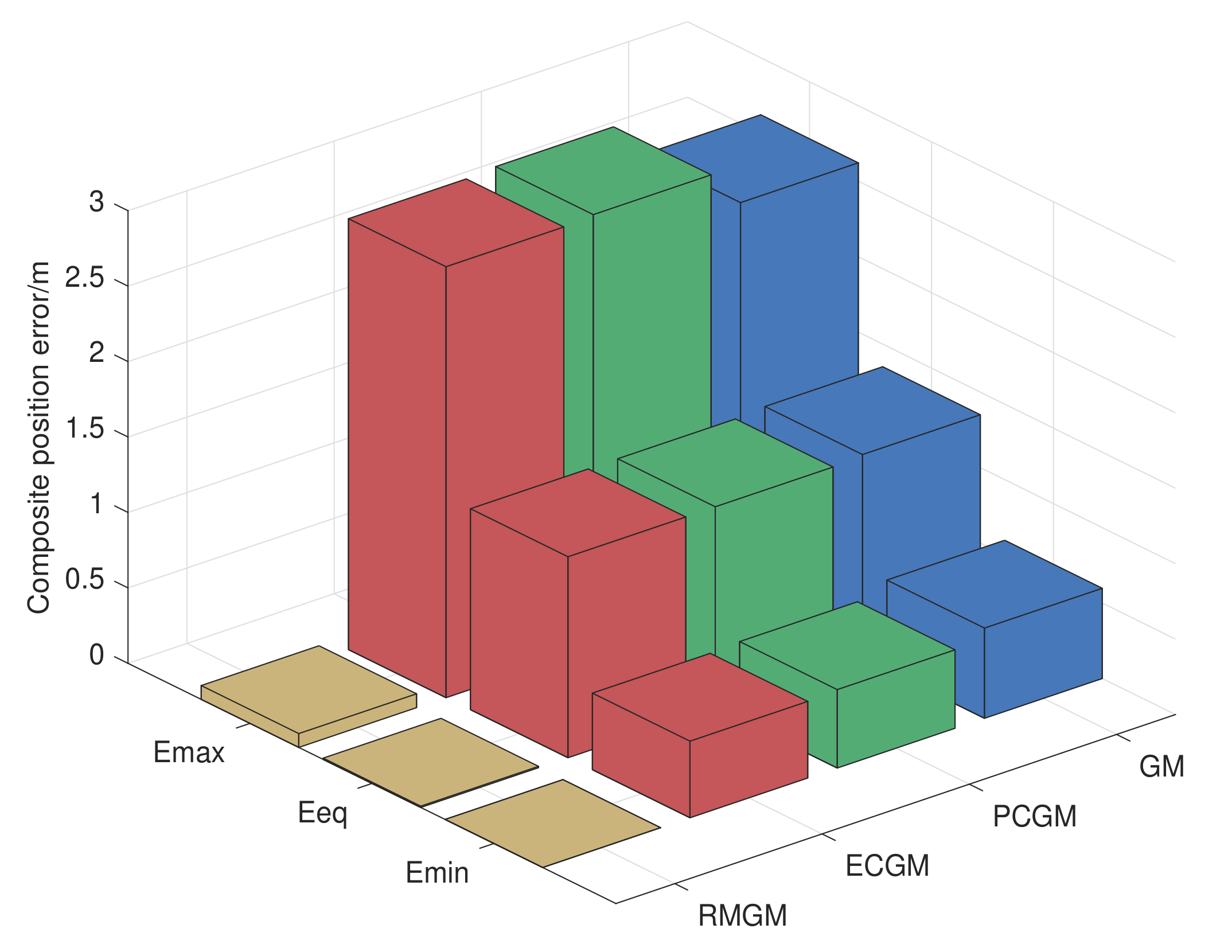
| Method | Emin | Eeq | Emax |
|---|---|---|---|
| RMGM | 0.0002 | 0.0112 | 0.1238 |
| ECGM | 0.4897 | 1.3459 | 2.6561 |
| PCGM | 0.4985 | 1.3476 | 2.6816 |
| GM | 0.5676 | 1.3595 | 2.5258 |
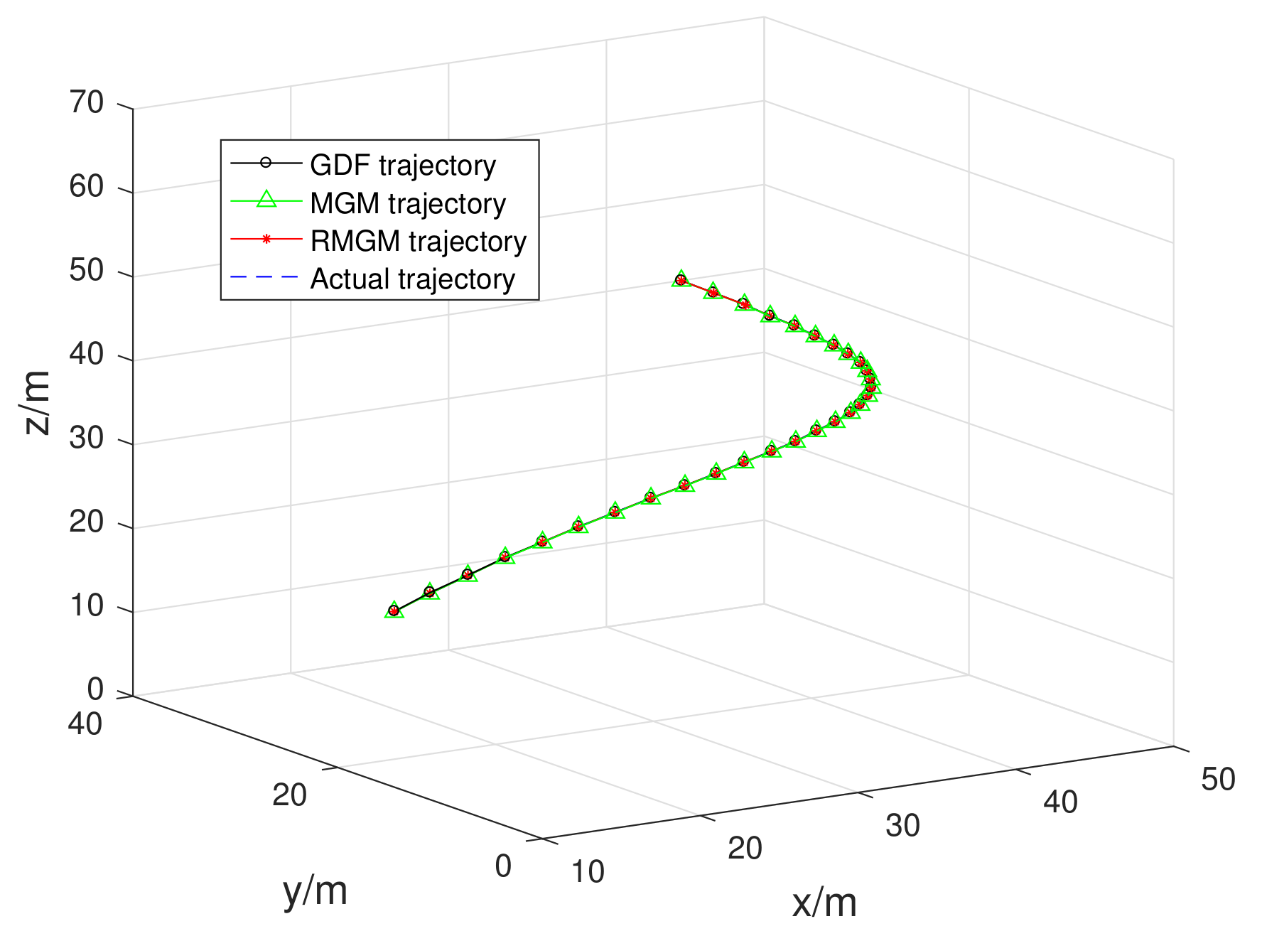
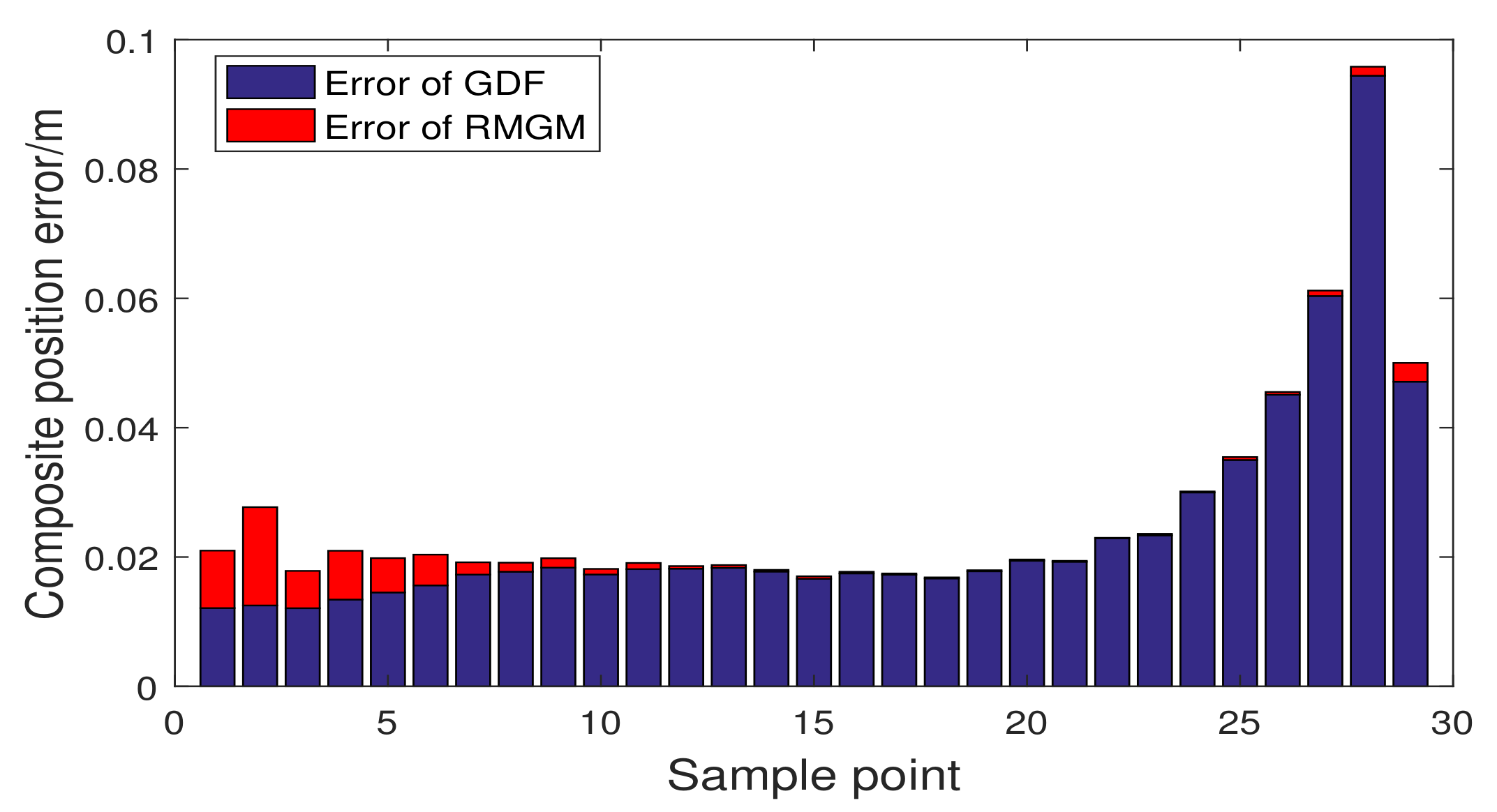
| Method | Emin | Eeq | Emax |
|---|---|---|---|
| MGM | 0.01531 | 0.03437 | 0.11419 |
| GDF | 0.01163 | 0.02435 | 0.09092 |
| RMGM | 0.00005 | 0.00273 | 0.01587 |
| Time | UAV Coordinates | Obstacle Coordinates | Prediction Coordinates | R1 | R2 | Adjusted Coordinate | R3 |
|---|---|---|---|---|---|---|---|
| 1 s | (20,40) | (52,40) | (45,40) | 17 | |||
| 2 s | (28,40) | (44,40) | (37.2,40) | 1.2 | 0 | (37.2,38) | 2.3 |
| 3 s | (36,40) | (36,40) | (29.4,40) | 14.6 | |||
| 4 s | (44,40) | (28,40) | (21.8,40) | 30.2 | |||
| 5 s | (52,40) | (20,40) | (14.3,40) |
| Time | UAV Coordinates | Obstacle Coordinates | Prediction Coordinates | R1 | R2 | Adjusted Coordinate | R3 |
|---|---|---|---|---|---|---|---|
| 1 s | (20,40) | (7,40) | (23.6,40) | 4.4 | |||
| 2 s | (28,40) | (23,40) | (32.2,40) | 3.8 | |||
| 3 s | (36,40) | (32,40) | (43.8,40) | 0.2 | 0 | (43.8,38) | 2.3 |
| 4 s | (44,40) | (44,40) | (59.2,40) | 7.2 | |||
| 5 s | (52,40) | (60,40) | (112,40) |
| Time | UAV Coordinates | Obstacle Coordinates | Prediction Coordinates | R1 | R2 | Adjusted Coordinate | R3 |
|---|---|---|---|---|---|---|---|
| 1 s | (20,40) | (39.5,28.6) | (37.7,34.3) | 11.25 | |||
| 2 s | (28,40) | (37.7,34.3) | (35.9,41) | 1 | 4.02 | (32,40) | |
| 3 s | (36,40) | (36,40) | (34.3,46.6) | 11.73 | |||
| 4 s | (44,40) | (33.6,46.4) | (31.4,53.8) | 24.80 | |||
| 5 s | (52,40) | (32.6,53.8) | (31.6,62.3) |
Publisher’s Note: MDPI stays neutral with regard to jurisdictional claims in published maps and institutional affiliations. |
© 2021 by the authors. Licensee MDPI, Basel, Switzerland. This article is an open access article distributed under the terms and conditions of the Creative Commons Attribution (CC BY) license (https://creativecommons.org/licenses/by/4.0/).
Share and Cite
Zhang, J.; Li, J.; Yang, H.; Feng, X.; Sun, G. Complex Environment Path Planning for Unmanned Aerial Vehicles. Sensors 2021, 21, 5250. https://doi.org/10.3390/s21155250
Zhang J, Li J, Yang H, Feng X, Sun G. Complex Environment Path Planning for Unmanned Aerial Vehicles. Sensors. 2021; 21(15):5250. https://doi.org/10.3390/s21155250
Chicago/Turabian StyleZhang, Jing, Jiwu Li, Hongwei Yang, Xin Feng, and Geng Sun. 2021. "Complex Environment Path Planning for Unmanned Aerial Vehicles" Sensors 21, no. 15: 5250. https://doi.org/10.3390/s21155250