Author Contributions
Conceptualisation, M.P. (Marcin Piekarczyk), K.R. and Ł.B.; methodology, M.P. (Marcin Piekarczyk) and K.R.; software, M.P. (Marcin Piekarczyk) and O.B.; validation, M.P. (Marcin Piekarczyk), Ł.B., K.R., O.B., S.S. and M.N.; formal analysis, Ł.B.; investigation, M.P. (Marcin Piekarczyk); resources, S.S. and M.N.; data curation, S.S. and M.N.; writing—original draft preparation, M.P. (Marcin Piekarczyk), Ł.B., K.R., O.B., S.S., T.A. and M.N.; writing—review and editing, N.M.B., D.E.A.-C., K.A.C., D.G., A.C.G., B.H., P.H., R.K., M.K. (Marcin Kasztelan), M.K. (Marek Knap), P.K., B.Ł., J.M., A.M., V.N., M.P. (Maciej Pawlik), M.R., O.S., K.S. (Katarzyna Smelcerz), K.S. (Karel Smolek), J.S., T.W., K.W.W., J.Z.-S. and T.A.; visualisation, O.B., M.N. and S.S.; supervision, M.P. (Marcin Piekarczyk) and Ł.B.; project administration, P.H., Ł.B. and M.P. (Marcin Piekarczyk); funding acquisition, P.H., M.P. (Marcin Piekarczyk) and Ł.B. All authors have read and agreed to the published version of the manuscript.
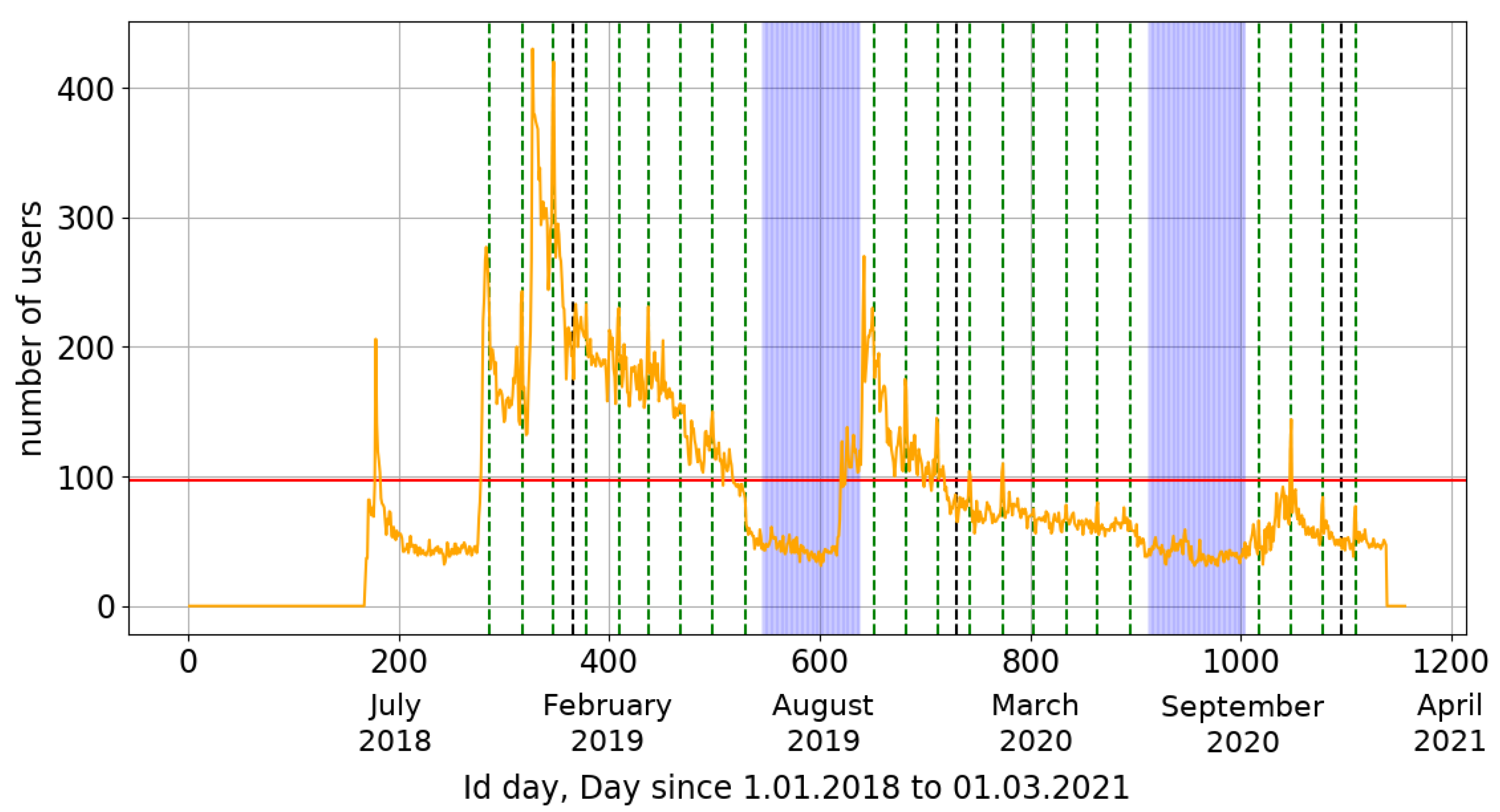
Figure 1.
Daily activity of the CREDO Detector application users from the premiere of the application (June 2018) to 1 March 2021. Green lines show the days of the event in the competition for schools. Dashed black lines indicate the beginning and end of a given year. Horizontal red line reflects the average daily number of active users (97). Blue areas indicate areas between two editions of the competition (early July to early October).
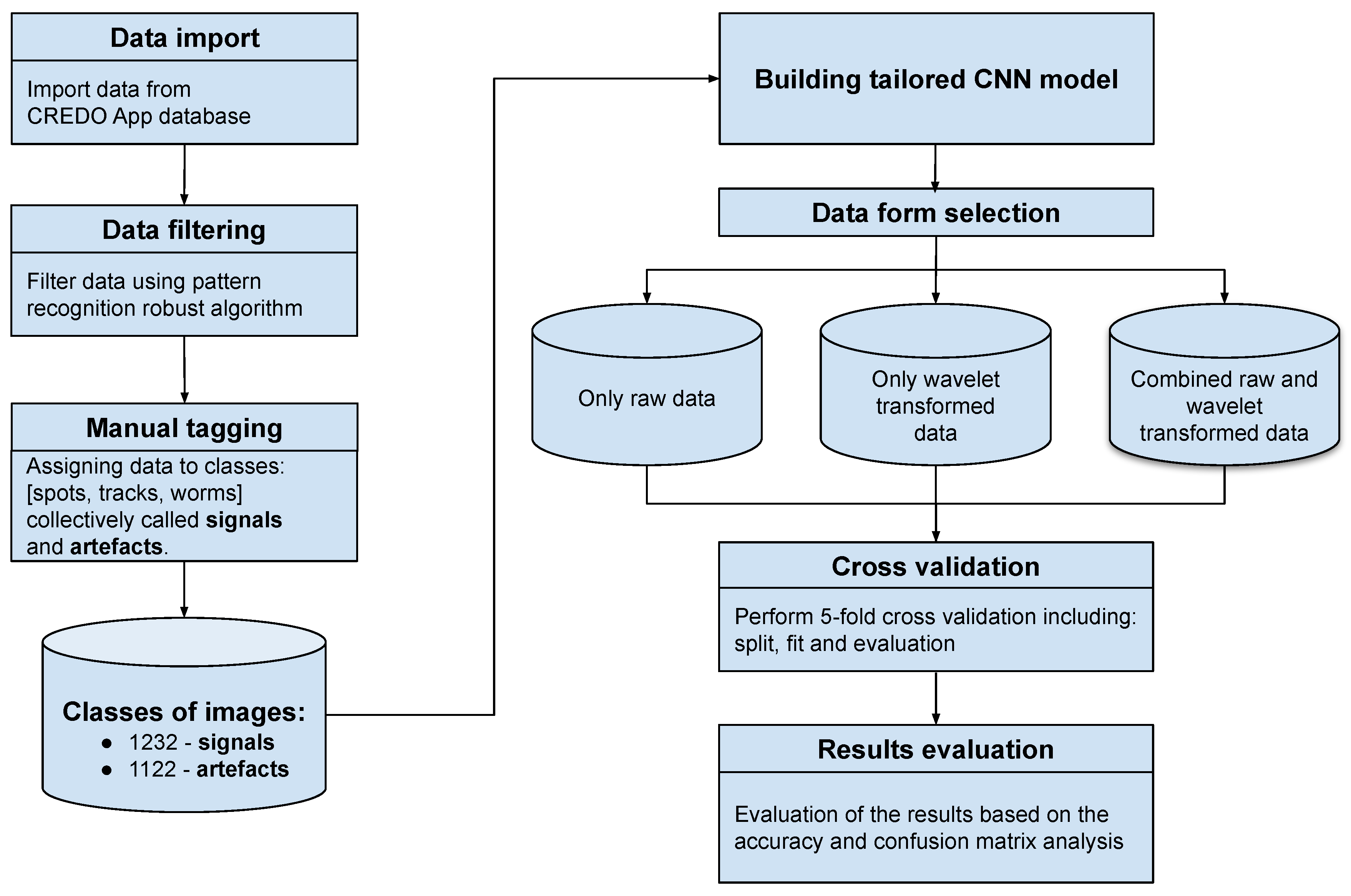
Figure 2.
Computation experiment flow chart.
Figure 2.
Computation experiment flow chart.
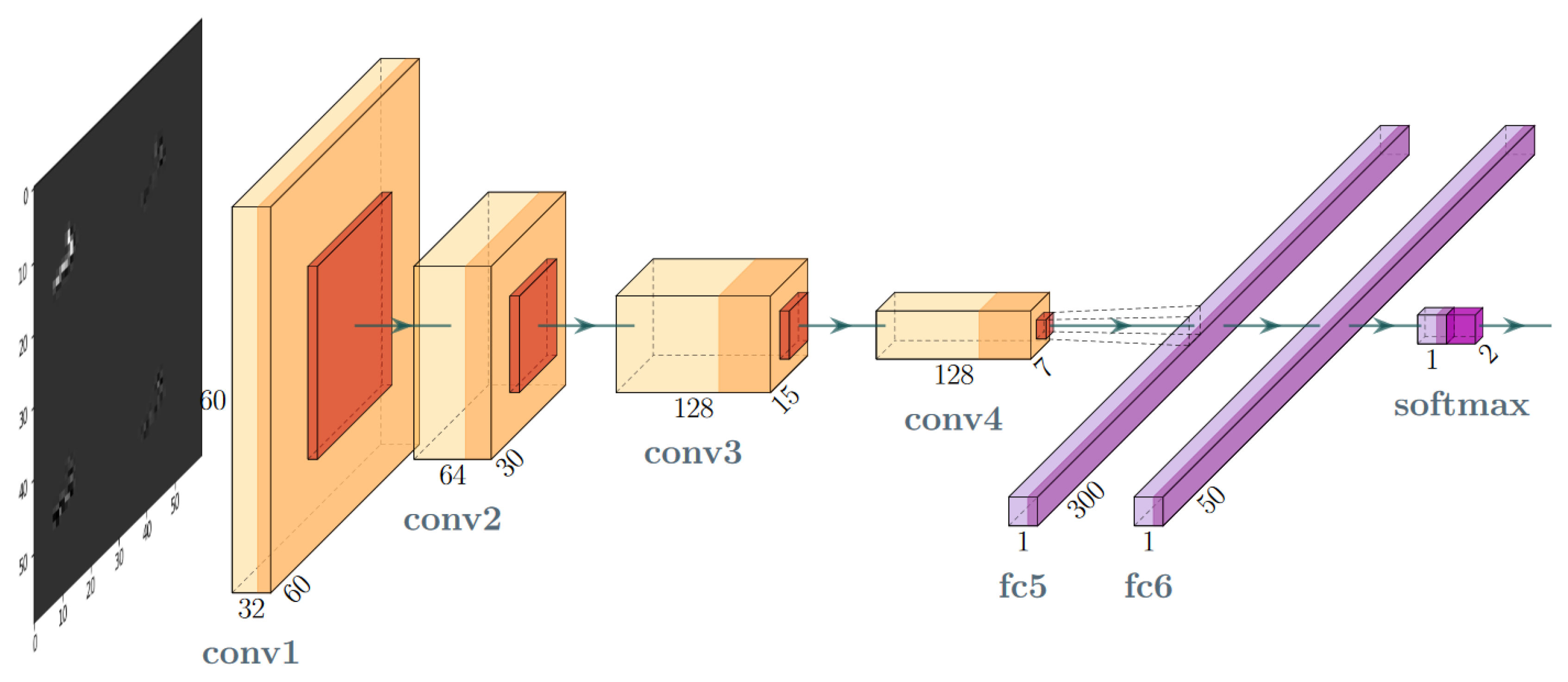
Figure 3.
Layer-oriented signal flow in the convolutional network (CNN) artefact filtration model.
Figure 3.
Layer-oriented signal flow in the convolutional network (CNN) artefact filtration model.
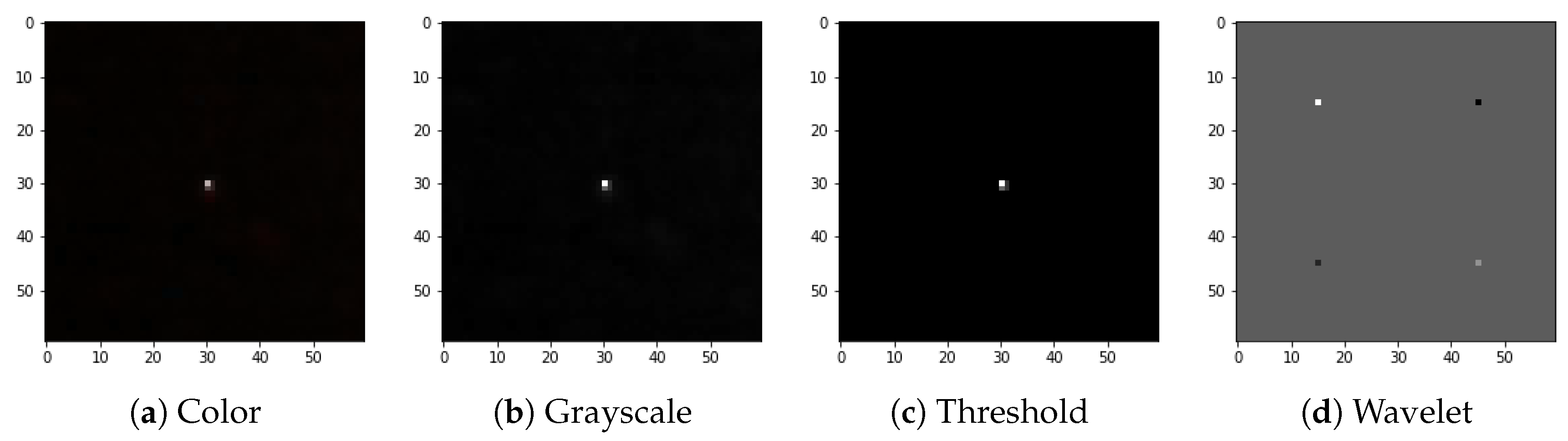
Figure 4.
Preprocessing flow: (a) color input image, (b) grayscale accumulation, (c) adaptive thresholding, (d) wavelet transformation. Example of the spot-type image.
Figure 4.
Preprocessing flow: (a) color input image, (b) grayscale accumulation, (c) adaptive thresholding, (d) wavelet transformation. Example of the spot-type image.
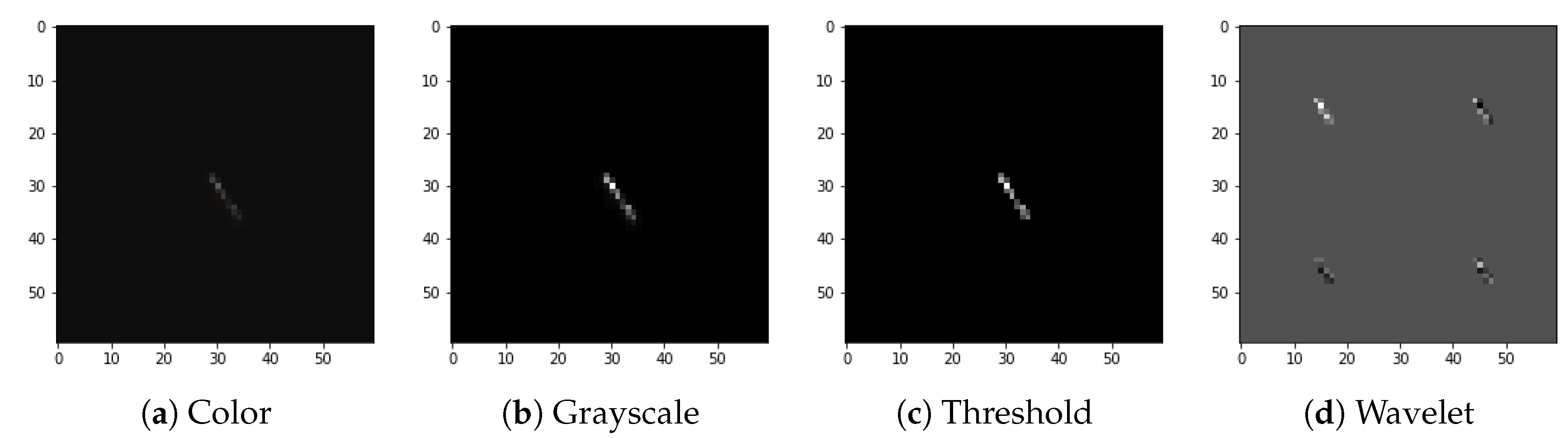
Figure 5.
Preprocessing flow: (a) color input image, (b) grayscale accumulation, (c) adaptive thresholding, (d) wavelet transformation. Example of the track-type image.
Figure 5.
Preprocessing flow: (a) color input image, (b) grayscale accumulation, (c) adaptive thresholding, (d) wavelet transformation. Example of the track-type image.
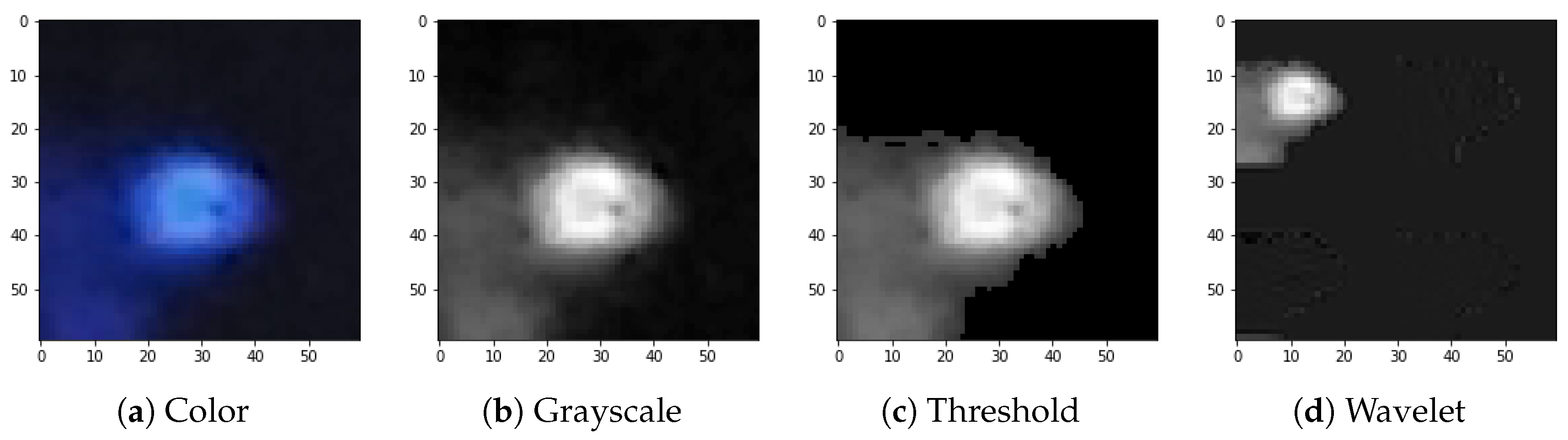
Figure 6.
Preprocessing flow: (a) color input image, (b) grayscale accumulation, (c) adaptive thresholding, (d) wavelet transformation. Example of the worm-type image.
Figure 6.
Preprocessing flow: (a) color input image, (b) grayscale accumulation, (c) adaptive thresholding, (d) wavelet transformation. Example of the worm-type image.
Figure 7.
Preprocessing flow: (a) color input image, (b) grayscale accumulation, (c) adaptive thresholding, (d) wavelet transformation. Example of the artefact image.
Figure 7.
Preprocessing flow: (a) color input image, (b) grayscale accumulation, (c) adaptive thresholding, (d) wavelet transformation. Example of the artefact image.
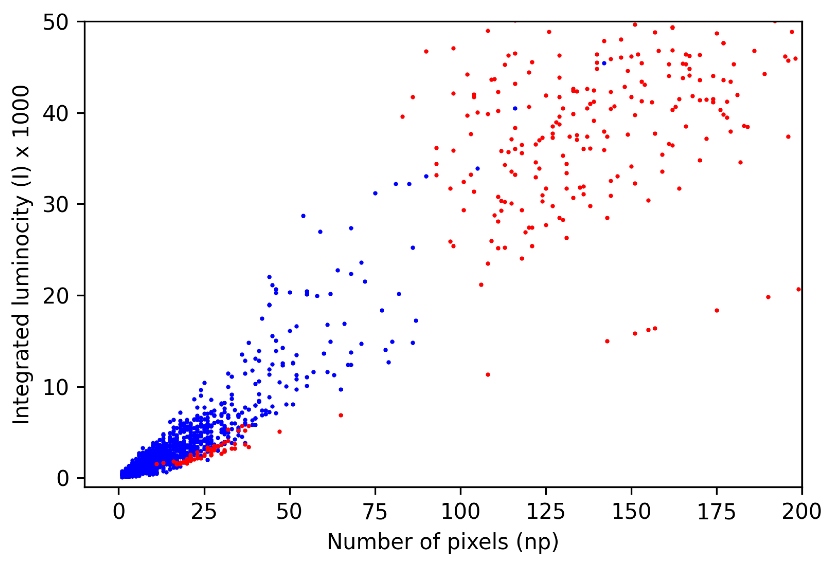
Figure 8.
Structural distribution of samples belonging to each class in the feature space (partially scaled-up key area). Points assigned to signals and artefacts are marked blue and red, respectively.
Figure 8.
Structural distribution of samples belonging to each class in the feature space (partially scaled-up key area). Points assigned to signals and artefacts are marked blue and red, respectively.
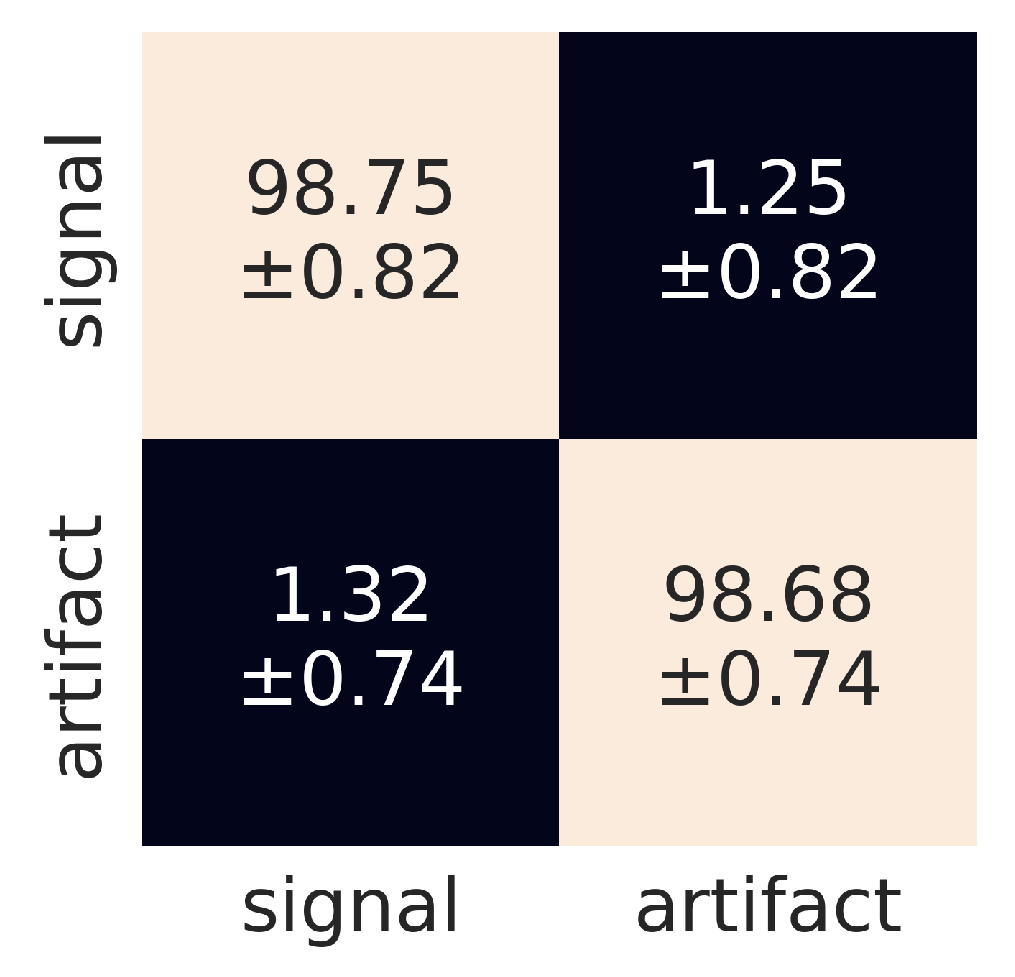
Figure 9.
Confusion matrix for the raw data. The horizontal and vertical dimensions refer to predicted and judged labels, respectively.
Figure 9.
Confusion matrix for the raw data. The horizontal and vertical dimensions refer to predicted and judged labels, respectively.
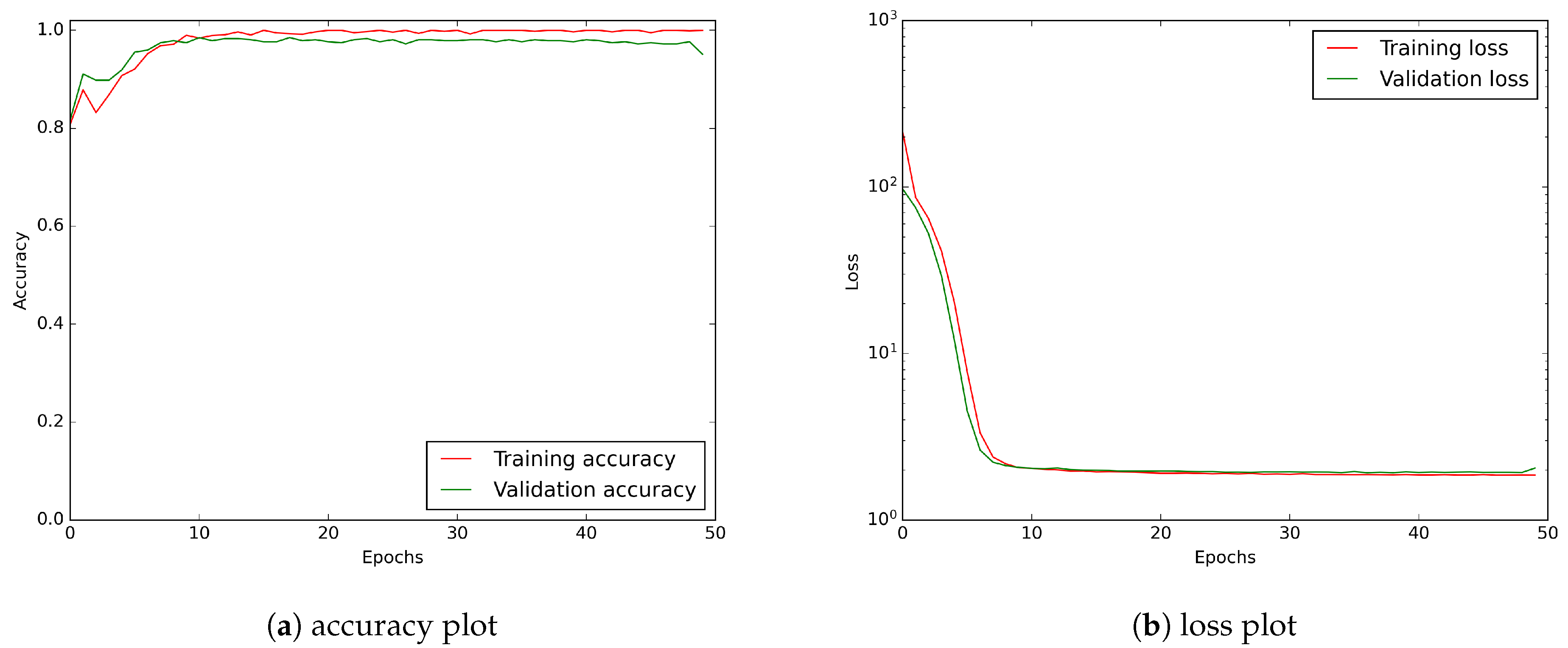
Figure 10.
CNN model learning history showing accuracy and loss curves. A logarithmic scale has been applied to the loss plot to keep a better visibility.
Figure 10.
CNN model learning history showing accuracy and loss curves. A logarithmic scale has been applied to the loss plot to keep a better visibility.
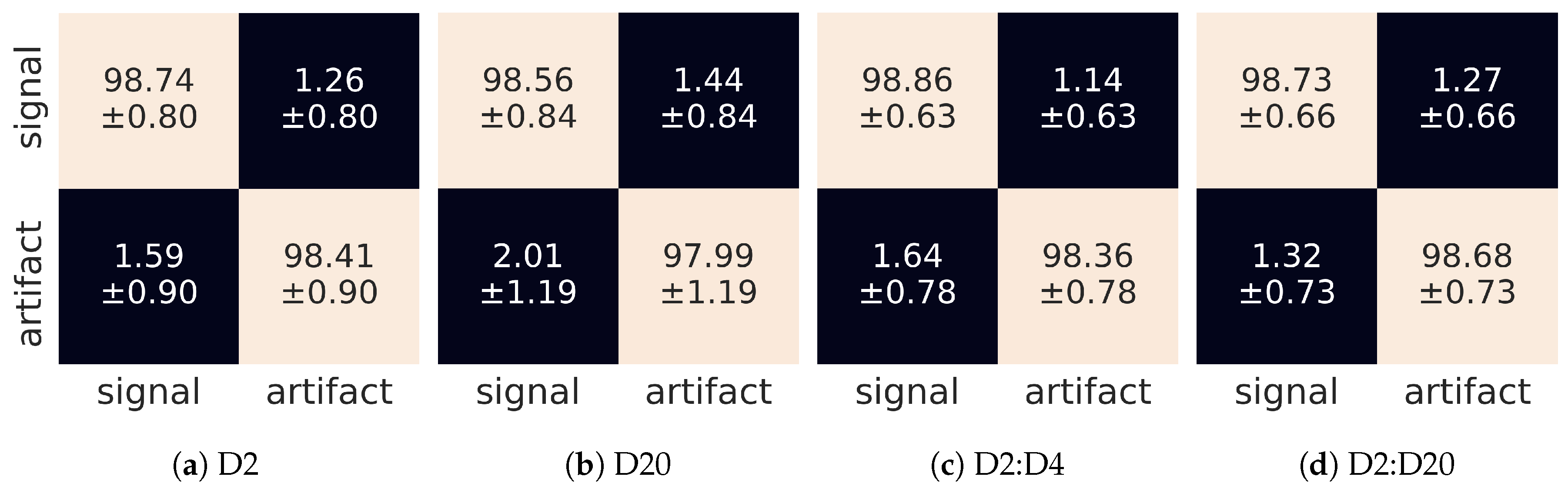
Figure 11.
Confusion matrices for different input tensors: (a) single D2 wavelet, (b) single D20 wavelet, (c) composition of [D2,D4] wavelets, (d) composition of [D2,D4,D6,...,D20] wavelets. The horizontal and vertical dimensions refer to predicted and judged labels, respectively.
Figure 11.
Confusion matrices for different input tensors: (a) single D2 wavelet, (b) single D20 wavelet, (c) composition of [D2,D4] wavelets, (d) composition of [D2,D4,D6,...,D20] wavelets. The horizontal and vertical dimensions refer to predicted and judged labels, respectively.
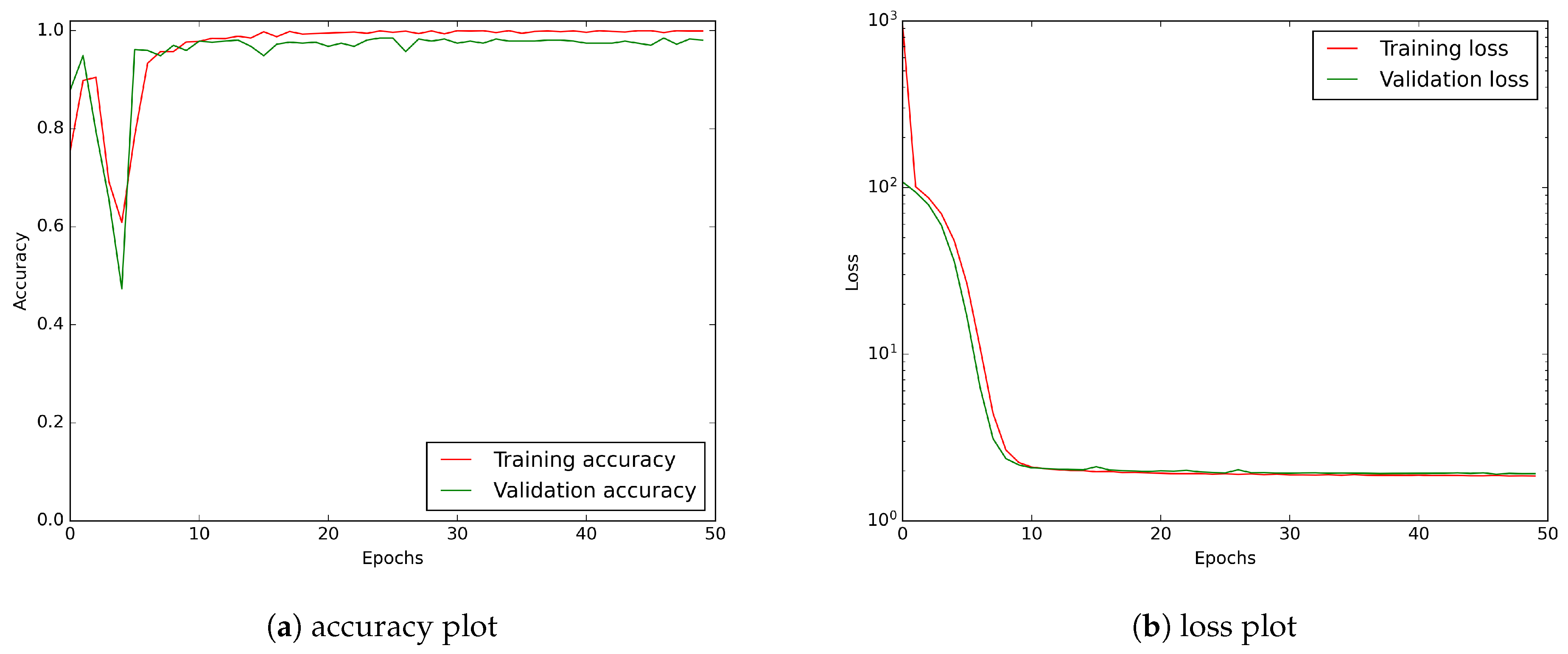
Figure 12.
The exemplary of CNN model learning history for input tensor consisting of D2:D20 wavelets: (a) accuracy plot, (b) loss curve. A logarithmic scale has been applied to the loss plot to keep a better visibility.
Figure 12.
The exemplary of CNN model learning history for input tensor consisting of D2:D20 wavelets: (a) accuracy plot, (b) loss curve. A logarithmic scale has been applied to the loss plot to keep a better visibility.
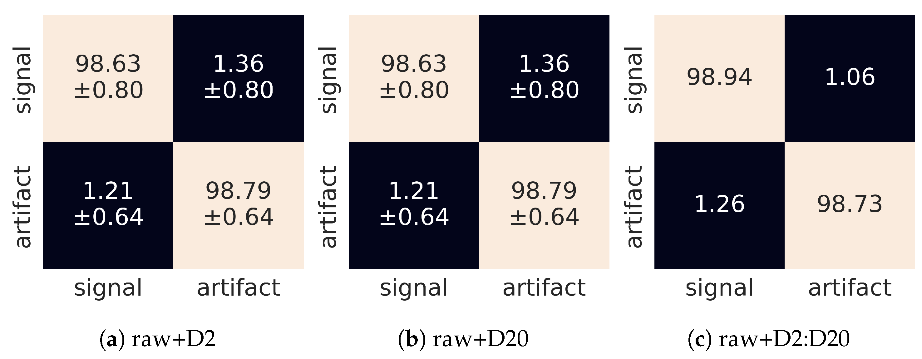
Figure 13.
Confusion matrices for different dimensions of the input tensors: (a) composition of the raw image and single D2 wavelet, (b) composition of the raw image and single D20 wavelet, (c) composition of the raw image and collection of [D2, D4, ..., D20] wavelets. The horizontal and vertical dimensions refer to predicted and judged labels, respectively.
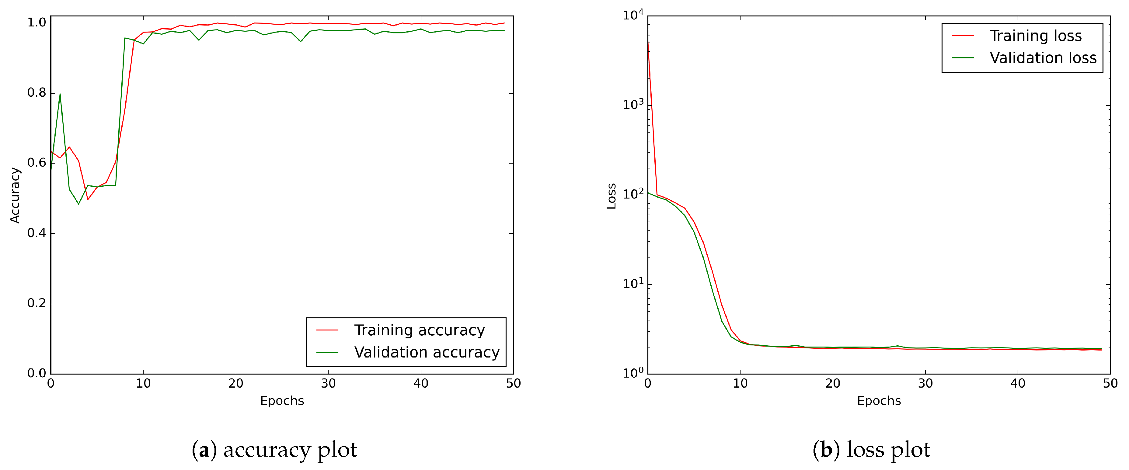
Figure 14.
CNN model learning history for an input tensor consisting of raw data merged with D2:20 wavelets: (a) accuracy plot, (b) loss curve. A logarithmic scale has been applied to the loss plot to keep a better visibility.
Figure 14.
CNN model learning history for an input tensor consisting of raw data merged with D2:20 wavelets: (a) accuracy plot, (b) loss curve. A logarithmic scale has been applied to the loss plot to keep a better visibility.
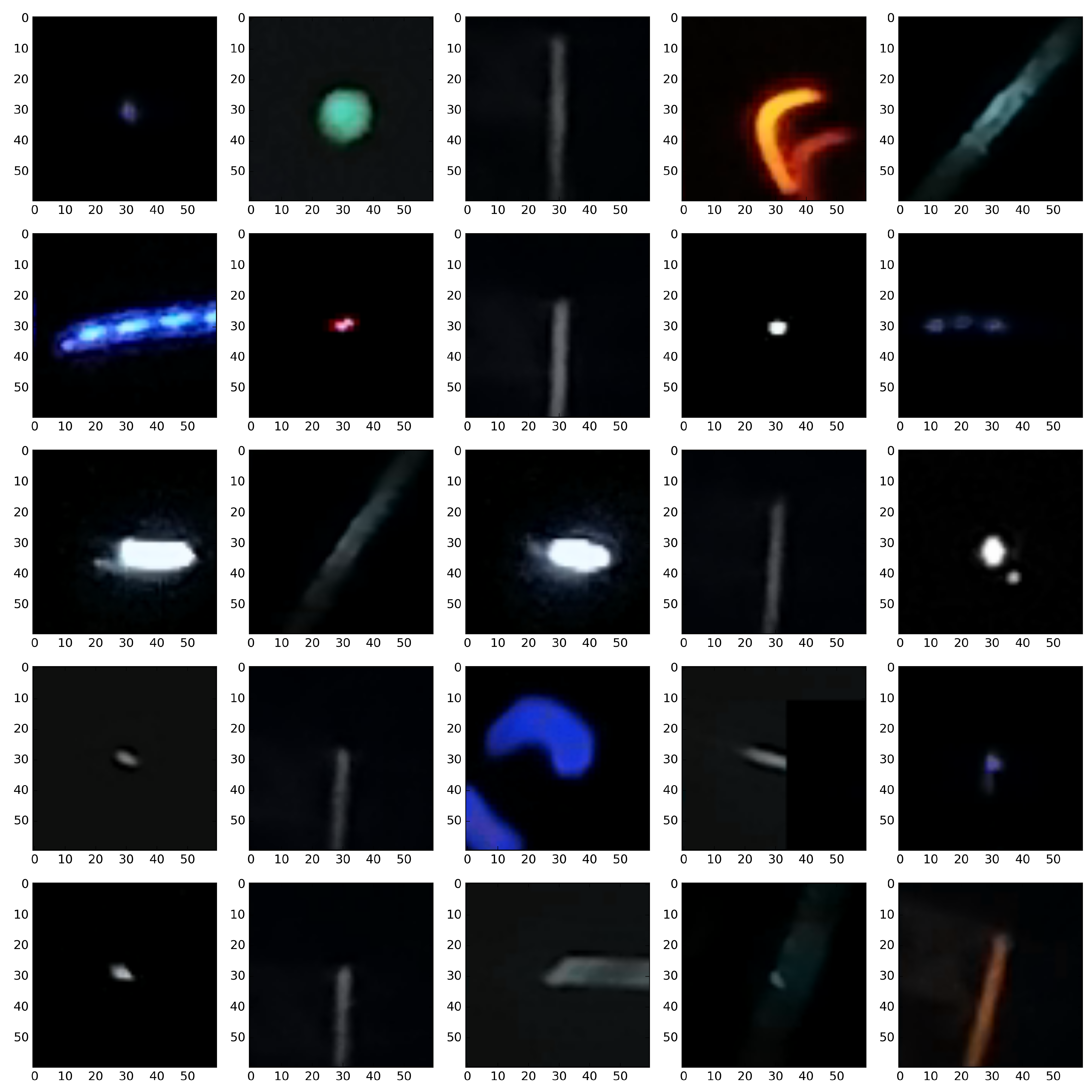
Figure 15.
Classification on the selected part of the original CREDO set demonstrating signal class. An example of the performance of a classifier based on a dimension 2 input tensor composed of the greyscale image and a D2 wavelet.
Figure 15.
Classification on the selected part of the original CREDO set demonstrating signal class. An example of the performance of a classifier based on a dimension 2 input tensor composed of the greyscale image and a D2 wavelet.
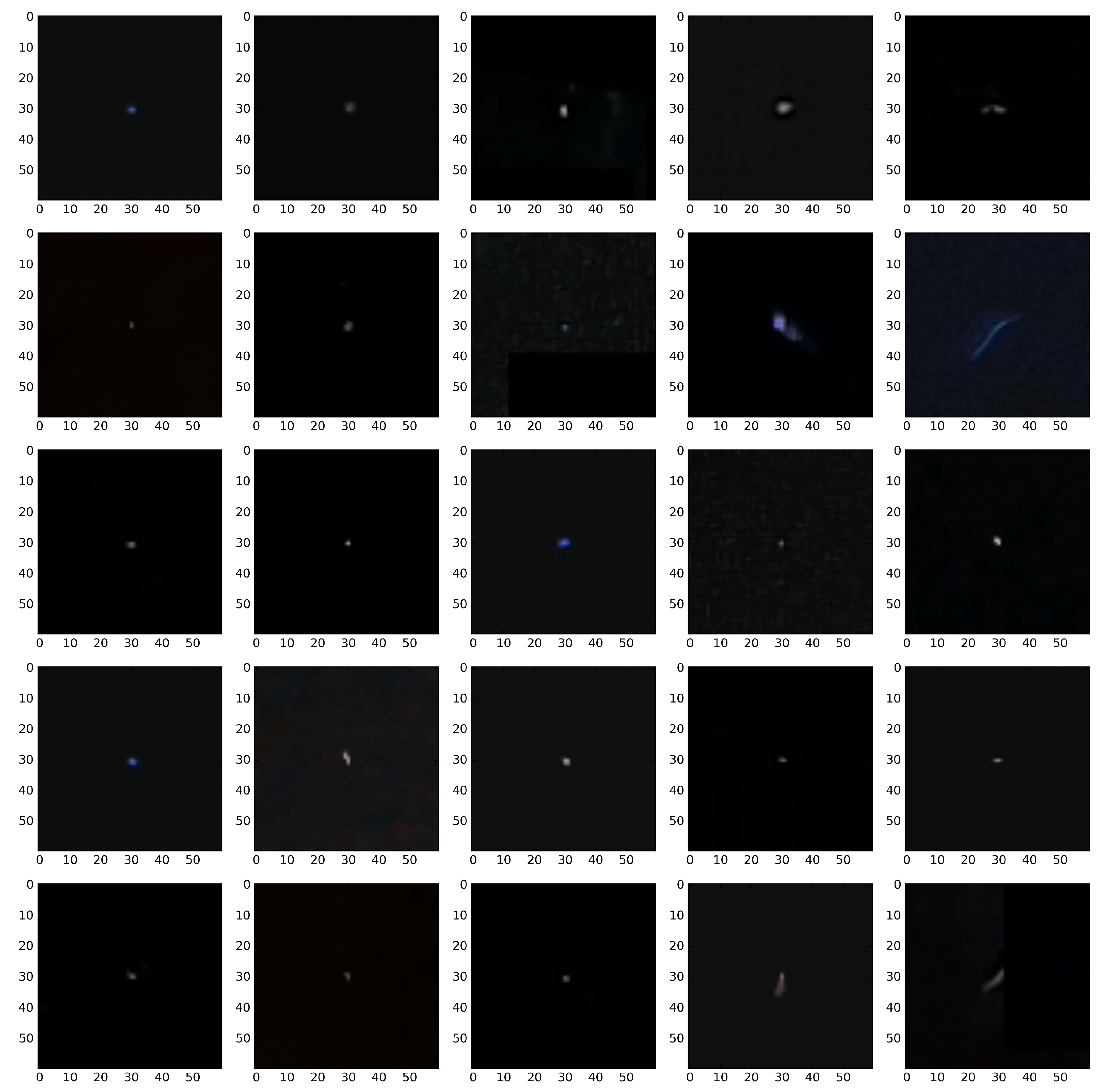
Figure 16.
Classification on the selected part of original CREDO set demonstrating the artefact class. An example of the performance of a classifier based on a dimension 2 input tensor composed of the greyscale image and a D2 wavelet.
Figure 16.
Classification on the selected part of original CREDO set demonstrating the artefact class. An example of the performance of a classifier based on a dimension 2 input tensor composed of the greyscale image and a D2 wavelet.
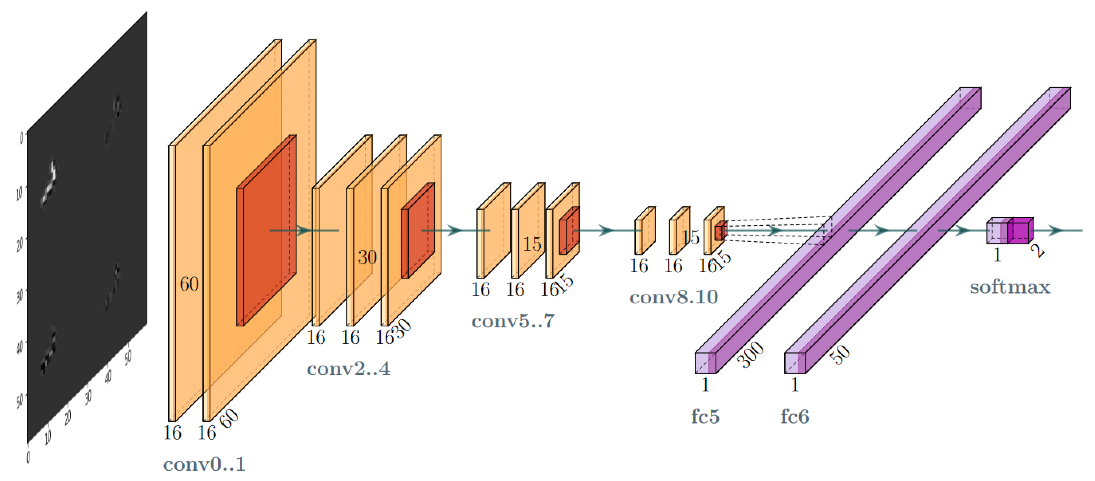
Figure 17.
Layer-oriented signal flow in the convolutional network (CNN) artefact filtration model of a smaller scale.
Figure 17.
Layer-oriented signal flow in the convolutional network (CNN) artefact filtration model of a smaller scale.
Table 1.
All participants vs. competition participants. Data collected from 1 October 2019 to 30 January 2020).
Table 1.
All participants vs. competition participants. Data collected from 1 October 2019 to 30 January 2020).
| | All | Competitors | (% of All) |
|---|
| Users | 1533 | 717 | (47%) |
| Teams | 310 | 62 | (21%) |
| Devices | 1756 | 836 | (48%) |
| Total time work [Hours] | 459,000 | 170,000 | (37%) |
| Candidates of detections | 1,207,000 | 812,000 | (67%) |
| Good Detections | 558,000 | 242,000 | (46%) |
| % of good candidates | 46% | 30% | |
Table 2.
Layer-by-layer summary of the proposed CNN model. Each layer name is given followed by the number of feature maps (convolutional layers) or neurons (dense layers), the size of the convolutional filter or pooling region, the activation function used and, last, the number of parameters to learn.
| Layer Type | Features | Size | Activation | Params |
|---|
| Convolution 2D | 32 | 5 × 5 | ReLU | 832 |
| Max Pooling | - | 2 × 2 | - | - |
| Convolution 2D | 64 | 5 × 5 | ReLU | 51,264 |
| Max Pooling | - | 2 × 2 | - | - |
| Convolution 2D | 128 | 5 × 5 | ReLU | 204,928 |
| Max Pooling | - | 2 × 2 | - | - |
| Convolution 2D | 128 | 5 × 5 | ReLU | 409,728 |
| Max Pooling | - | 2 × 2 | - | - |
| Flatten | 1152 | - | - | - |
| Dense | 300 | - | ReLU | 345,900 |
| Dense | 50 | - | ReLU | 15,050 |
| Dense | 2 | - | Softmax | 102 |
| Total params: 1,027,804 |
| Trainable params: 1,027,804 |
| Non-trainable params: 0 |
Table 3.
Performance of the base model applied to the input data. Three variants of classifiers using manually selected two features were analysed: a simple heuristic model based on decision rules, a kNN type classifier (k = 7, metric = L2) and a classifier based on boosted decision trees called random forests (number_estimators = 100, depth_trees = 2). Results have been estimated using repeated k-fold validation (5 rounds with 5 folds each).
| Type | Overall Acc ± Std Dev | Signal Acc ± Std Dev | Artefact Acc ± Std Dev |
|---|
| Baseline trigger | 96.87 ± 0.66 | 98.65 ± 1.10 | 94.92 ± 1.14 |
| Nearest Neighbor | 96.40 ± 0.73 | 98.57 ± 0.60 | 94.01 ± 1.27 |
| Random Forest | 97.07 ± 0.77 | 99.17 ± 0.73 | 94.76 ± 1.39 |
Table 4.
CNN model performance for raw data set. Results have been estimated using repeated k-fold validation (5 rounds with 5 folds each).
Table 4.
CNN model performance for raw data set. Results have been estimated using repeated k-fold validation (5 rounds with 5 folds each).
| Tensor Depth | Overall Acc ± Std Dev | Signal Acc ± Std Dev | Artefact Acc ± Std Dev |
|---|
| 3 | 98.71± 0.50 | 98.75 ± 0.82 | 98.68 ± 0.74 |
Table 5.
CNN model performance for various single wavelet transformations applied to input data. Results have been estimated using repeated k-fold validation (5 rounds with 5 folds each).
Table 5.
CNN model performance for various single wavelet transformations applied to input data. Results have been estimated using repeated k-fold validation (5 rounds with 5 folds each).
| Wavelet | Tensor | Overall Acc | Signal Acc | Artefact Acc |
|---|
| Number | Depth | ± Std Dev | ± Std Dev | ± Std Dev |
|---|
| D2 | 1 | 98.56 ± 0.62 | 98.74 ± 0.80 | 98.41 ± 0.90 |
| D4 | 1 | 98.54 ± 0.48 | 98.51 ± 0.86 | 98.45 ± 0.99 |
| D6 | 1 | 98.48 ± 0.46 | 98.51 ± 0.86 | 98.45 ± 0.99 |
| D8 | 1 | 98.48 ± 0.46 | 98.51 ± 0.86 | 98.45 ± 0.99 |
| D10 | 1 | 98.62 ± 0.49 | 99.01 ± 0.66 | 98.22 ± 0.78 |
| D12 | 1 | 98.63 ± 0.49 | 98.88 ± 0.69 | 98.34 ± 0.73 |
| D14 | 1 | 98.53 ± 0.56 | 98.60 ± 0.91 | 98.45 ± 0.83 |
| D16 | 1 | 98.44 ± 0.56 | 98.60 ± 0.91 | 98.45 ± 0.83 |
| D18 | 1 | 98.38 ± 0.40 | 98.49 ± 0.64 | 98.25 ± 0.94 |
| D20 | 1 | 98.28 ± 0.57 | 98.55 ± 0.83 | 97.99 ± 1.19 |
Table 6.
CNN model performance for various wavelet transformations applied to input data (deep tensors). Results have been estimated using repeated k-fold validation (5 rounds with 5 folds each).
Table 6.
CNN model performance for various wavelet transformations applied to input data (deep tensors). Results have been estimated using repeated k-fold validation (5 rounds with 5 folds each).
| Wavelets | Tensor | Overall Acc | Signal Acc | Artefact Acc |
|---|
| Sequence | Depth | ± Std Dev | ± Std Dev | ± Std Dev |
|---|
| D2:D4 | 2 | 98.62 ± 0.41 | 98.86 ± 0.63 | 98.36 ± 1.64 |
| D2:D6 | 3 | 98.65 ± 0.54 | 98.62 ± 0.77 | 98.68 ± 0.85 |
| D2:D8 | 4 | 98.65 ± 0.54 | 98.62 ± 0.62 | 98.68 ± 0.92 |
| D2:D10 | 5 | 98.71 ± 0.49 | 98.83 ± 0.74 | 98.57 ± 0.65 |
| D2:D12 | 6 | 98.60 ± 0.39 | 98.75 ± 0.85 | 98.43 ± 0.92 |
| D2:D14 | 7 | 98.67 ± 0.40 | 99.01 ± 0.67 | 98.29 ± 0.76 |
| D2:D16 | 8 | 98.64 ± 0.50 | 98.83 ± 0.68 | 98.43 ± 0.88 |
| D2:D18 | 9 | 98.73 ± 0.47 | 98.86 ± 0.83 | 98.59 ± 0.83 |
| D2:D20 | 10 | 98.71 ± 0.47 | 98.73 ± 0.66 | 98.68 ± 0.73 |
Table 7.
CNN model performance for raw data combined with wavelet set. Results have been estimated using repeated k-fold validation (5 rounds with 5 folds each).
Table 7.
CNN model performance for raw data combined with wavelet set. Results have been estimated using repeated k-fold validation (5 rounds with 5 folds each).
| Data | Tensor | Overall Acc | Signal Acc | Artefact Acc |
|---|
| Set | Depth | ± Std Dev | ± Std Dev | ± Std Dev |
|---|
| raw + D2 | 2 | 98.93 ± 0.39 | 98.99 ± 0.63 | 98.86 ± 0.67 |
| raw + D20 | 2 | 98.71 ± 0.43 | 98.64 ± 0.80 | 98.79 ± 0.64 |
| raw + D2:D20 | 11 | 98.84 ± 0.55 | 98.94 ± 0.71 | 98.73 ± 0.95 |
Table 8.
CNN model timing for different type of input data, where denotes the original RGB image and means Daubechies wavelet with length of n. To obtain statistically reliable results, classification time was measured for samples and then averaged.
Table 8.
CNN model timing for different type of input data, where denotes the original RGB image and means Daubechies wavelet with length of n. To obtain statistically reliable results, classification time was measured for samples and then averaged.
| Data Set | Tensor Depth | Learning Time [s] | Prediction Time [s] |
|---|
| for 50 Epochs | for Single Image |
|---|
| raw | 3 | 27 | 100 |
| D2 | 1 | 29 | 110 |
| raw + D2 | 4 | 29 | 140 |
| raw + D2:D10 | 8 | 33 | 180 |
| raw + D2:D20 | 13 | 39 | 260 |
Table 9.
Base CNN model performance for various single wavelet transformations applied to input data. Input tensor composed of a greyscale image and wavelet image components (a, v, h, d) set in a sequence which gives a tensor depth of 1 + 4. Results have been estimated using repeated k-fold validation (5 rounds with 5 folds each).
| Wavelet | Tensor | Overall Acc | Signal Acc | Artefact Acc |
|---|
| Number | Depth | ± Std Dev | ± Std Dev | ± Std Dev |
|---|
| raw + D2 | 5 | 98.11 ± 0.61 | 97.92 ± 0.91 | 98.32 ± 1.09 |
| raw + D4 | 5 | 98.10 ± 0.49 | 97.71 ± 0.86 | 98.54 ± 0.66 |
| raw + D6 | 5 | 97.92 ± 0.69 | 97.84 ± 0.96 | 97.90 ± 1.17 |
| raw + D8 | 5 | 97.99 ± 0.56 | 97.95 ± 1.01 | 98.02 ± 1.11 |
| raw + D10 | 5 | 98.03 ± 0.55 | 98.02 ± 0.96 | 98.04 ± 0.91 |
| raw + D12 | 5 | 98.10 ± 0.65 | 97.79 ± 1.06 | 98.43 ± 0.89 |
| raw + D14 | 5 | 98.10 ± 0.57 | 98.26 ± 0.85 | 97.90 ± 0.81 |
| raw + D16 | 5 | 98.13 ± 0.52 | 98.18 ± 0.58 | 98.07 ± 0.97 |
| raw + D18 | 5 | 97.95 ± 0.56 | 97.97 ± 0.78 | 97.93 ± 1.23 |
| raw + D20 | 5 | 98.04 ± 0.46 | 98.07 ± 0.70 | 98.00 ± 0.73 |
Table 10.
Layer-by-layer summary of the proposed smaller-scale CNN model. Each layer name is given followed by the number of feature maps (convolutional layers) or neurons (dense layers), the size of the convolutional filter or pooling region, the activation function used and, last, the number of parameters to learn.
| Layer Type | Features | Size | Activation | Params |
|---|
| Convolution 2D | 16 | 3 × 3 | ReLU | 736 |
| Convolution 2D | 16 | 5 × 5 | ReLU | 6416 |
| Max Pooling | - | 2 × 2 | - | - |
| Convolution 2D | 16 | 3 × 3 | ReLU | 2320 |
| Convolution 2D | 16 | 3 × 3 | ReLU | 2320 |
| Convolution 2D | 16 | 5 × 5 | ReLU | 6416 |
| Max Pooling | - | 2 ×2 | - | - |
| Convolution 2D | 16 | 3 × 3 | ReLU | 2320 |
| Convolution 2D | 16 | 3 × 3 | ReLU | 2320 |
| Convolution 2D | 16 | 5 × 5 | ReLU | 6416 |
| Max Pooling | - | 2 × 2 | - | - |
| Convolution 2D | 16 | 3 × 3 | ReLU | 2320 |
| Convolution 2D | 16 | 3 × 3 | ReLU | 2320 |
| Convolution 2D | 16 | 5 × 5 | ReLU | 6416 |
| Max Pooling | - | 2 × 2 | - | - |
| Flatten | 144 | - | - | - |
| Dense | 300 | - | ReLU | 43,500 |
| Dense | 50 | - | ReLU | 15,050 |
| Dense | 2 | - | Softmax | 102 |
| Total params: 98,972 |
| Trainable params: 98,972 |
| Non-trainable params: 0 |
Table 11.
Smaller-scale CNN model performance for various single wavelet transformations applied to input data. Results have been estimated using repeated k-fold validation (5 rounds with 5 folds each).
Table 11.
Smaller-scale CNN model performance for various single wavelet transformations applied to input data. Results have been estimated using repeated k-fold validation (5 rounds with 5 folds each).
| Wavelet | Tensor | Overall Acc | Signal Acc | Artefact Acc |
|---|
| Number | Depth | ± Std Dev | ± Std Dev | ± Std Dev |
|---|
| raw + D2 | 2 | 98.33 ± 0.58 | 98.49 ± 0.67 | 98.15 ± 1.14 |
| raw + D4 | 2 | 98.12 ± 0.88 | 98.33 ± 1.02 | 97.90 ± 1.22 |
| raw + D6 | 2 | 98.26 ± 0.48 | 98.41 ± 0.69 | 98.09 ± 0.89 |
| raw + D8 | 2 | 98.38 ± 0.60 | 98.46 ± 1.08 | 98.29 ± 0.80 |
| raw + D10 | 2 | 98.27 ± 0.48 | 98.59 ± 0.65 | 97.91 ± 0.84 |
| raw + D12 | 2 | 98.30 ± 0.61 | 98.52 ± 0.82 | 98.06 ± 1.06 |
| raw + D14 | 2 | 98.13 ± 0.55 | 98.28 ± 0.71 | 97.97 ± 0.96 |
| raw + D16 | 2 | 98.18 ± 0.53 | 98.36 ± 0.86 | 97.99 ± 0.89 |
| raw + D18 | 2 | 98.14 ± 0.57 | 98.10 ± 0.98 | 98.18 ± 0.85 |
| raw + D20 | 2 | 98.17 ± 0.54 | 98.30 ± 0.83 | 98.04 ± 0.73 |
Table 12.
Smaller-scale CNN model performance for various single wavelet transformations applied to input data. Input tensor composed of a greyscale image and wavelet image components (a, v, h, d) set in a sequence which gives a tensor depth of 1 + 4. Results have been estimated using repeated k-fold validation (5 rounds with 5 folds each).
| Wavelet | Tensor | Overall Acc | Signal Acc | Artefact Acc |
|---|
| Number | Depth | ± Std Dev | ± Std Dev | ± Std Dev |
|---|
| raw + D2 | 5 | 98.16 ± 0.54 | 98.10 ± 0.88 | 98.22 ± 0.89 |
| raw + D4 | 5 | 98.10 ± 0.48 | 98.02 ± 0.82 | 98.20 ± 0.84 |
| raw + D6 | 5 | 97.99 ± 0.54 | 97.99 ± 0.88 | 98.00 ± 1.10 |
| raw + D8 | 5 | 98.02 ± 0.35 | 97.89 ± 0.93 | 98.18 ± 0.94 |
| raw + D10 | 5 | 97.87 ± 0.64 | 97.74 ± 0.97 | 98.00 ± 0.92 |
| raw + D12 | 5 | 97.91 ± 0.69 | 97.82 ± 1.05 | 98.00 ± 0.86 |
| raw + D14 | 5 | 97.82 ± 0.61 | 97.94 ± 1.08 | 97.68 ± 1.11 |
| raw + D16 | 5 | 97.99 ± 0.58 | 98.04 ± 0.99 | 97.95 ± 0.96 |
| raw + D18 | 5 | 97.99 ± 0.42 | 97.68 ± 1.12 | 97.91 ± 1.10 |
| raw + D20 | 5 | 97.86 ± 0.59 | 97.79 ± 1.03 | 97.93 ± 0.86 |


 ,
, 


