
Virtual Electric Dipole Field Applied to Autonomous Formation Flight Control of Unmanned Aerial Vehicles


Abstract
:1. Introduction
2. Research Object
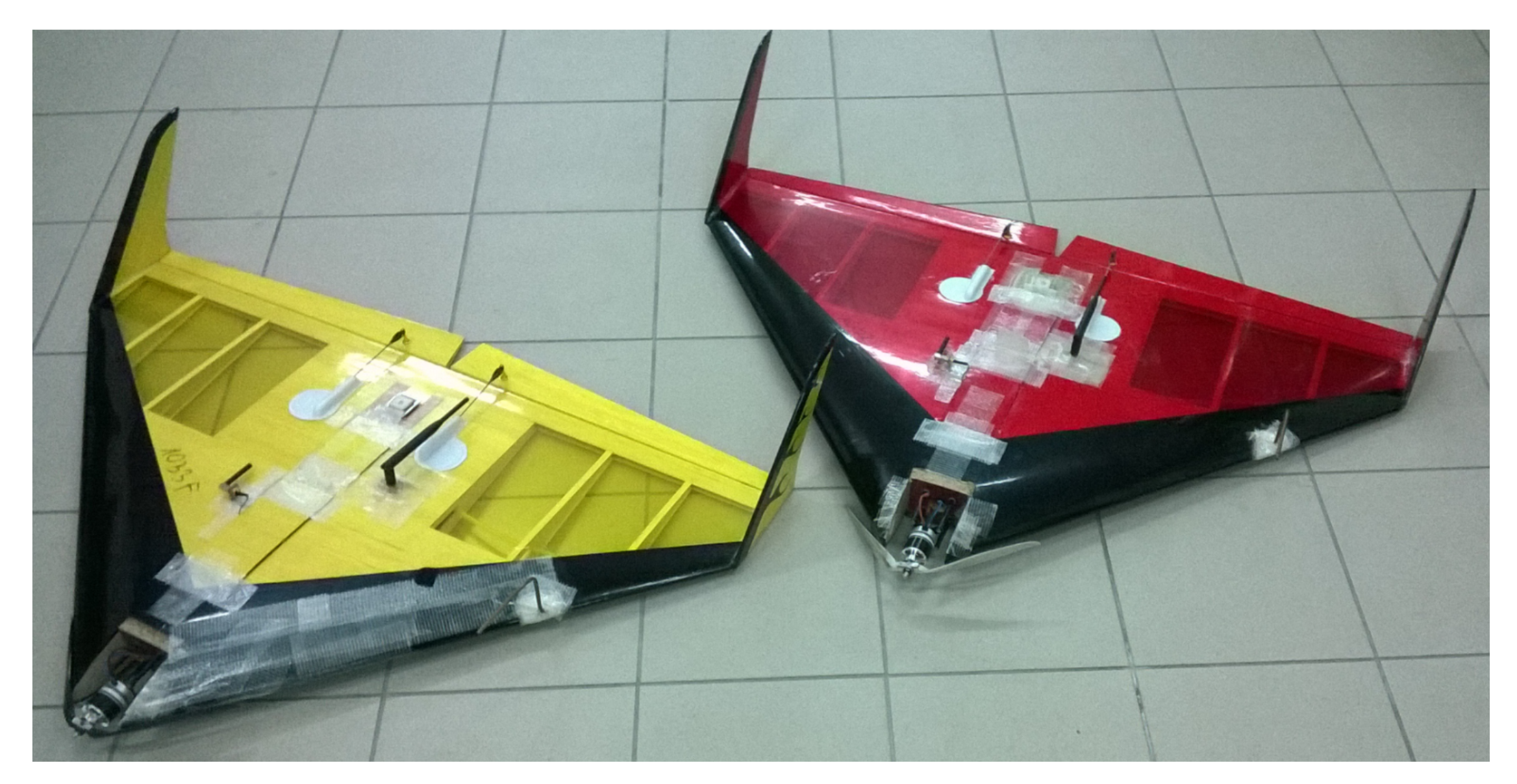
2.1. The Bullit 60
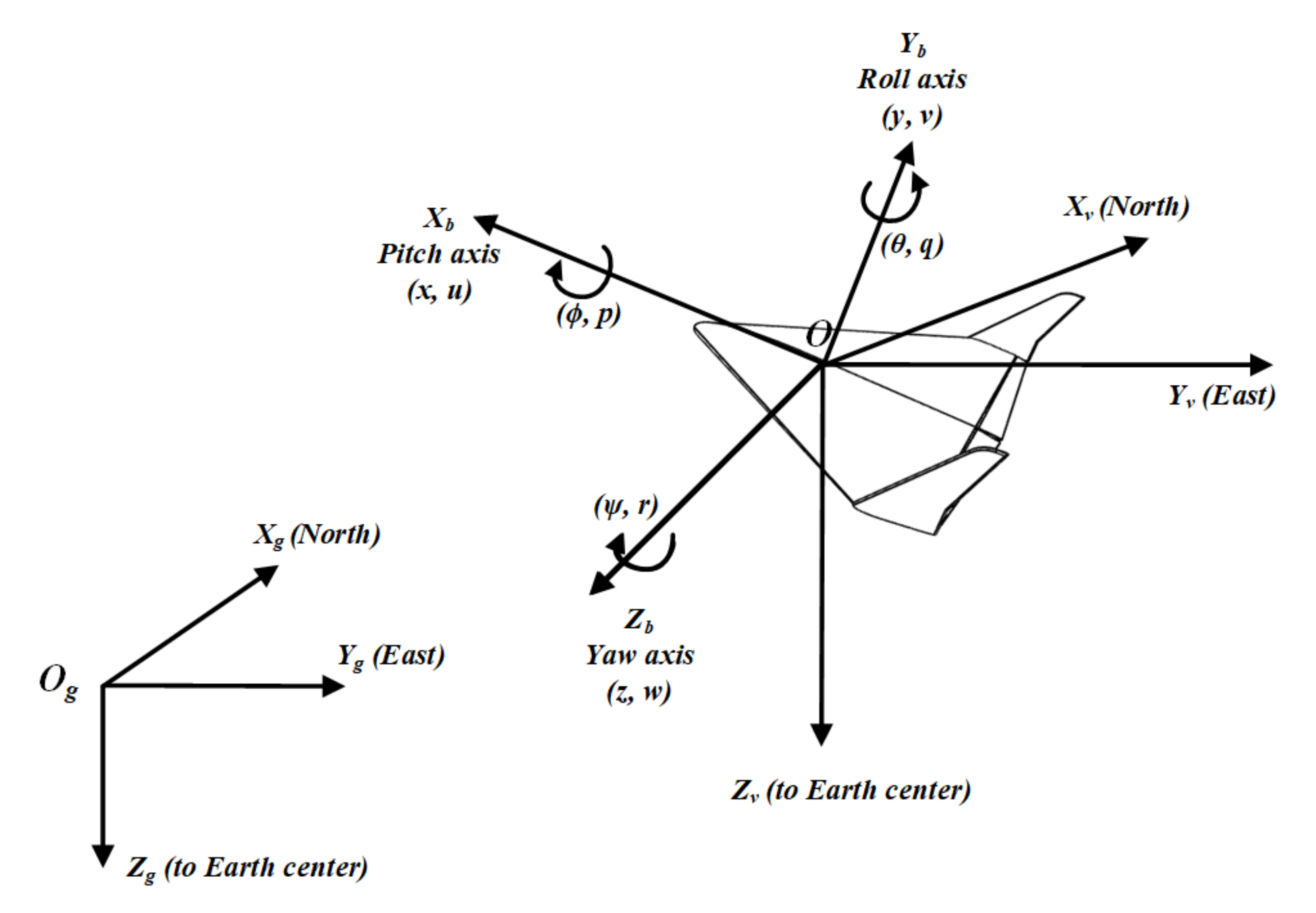
2.2. Mathematical Model
2.3. MAV Simulation System
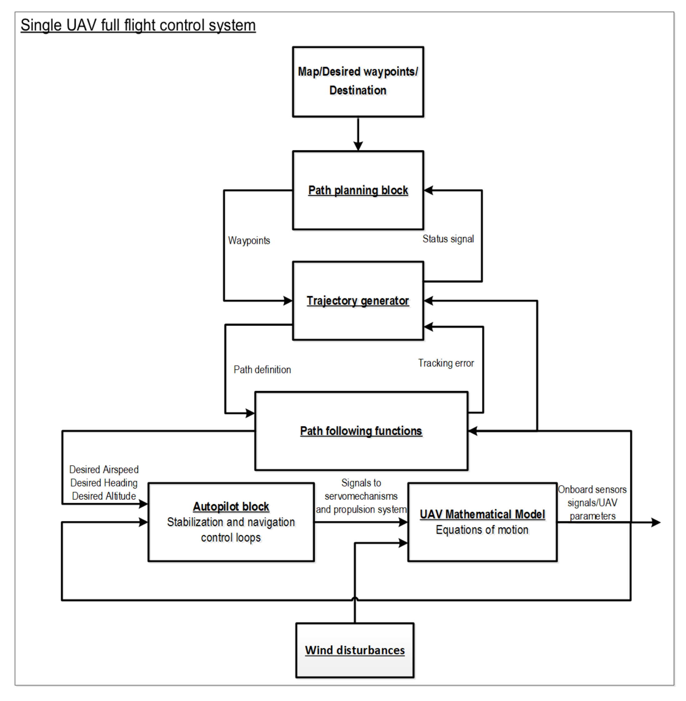
3. Virtual Electric Dipole Field for Autonomous Formation Flight
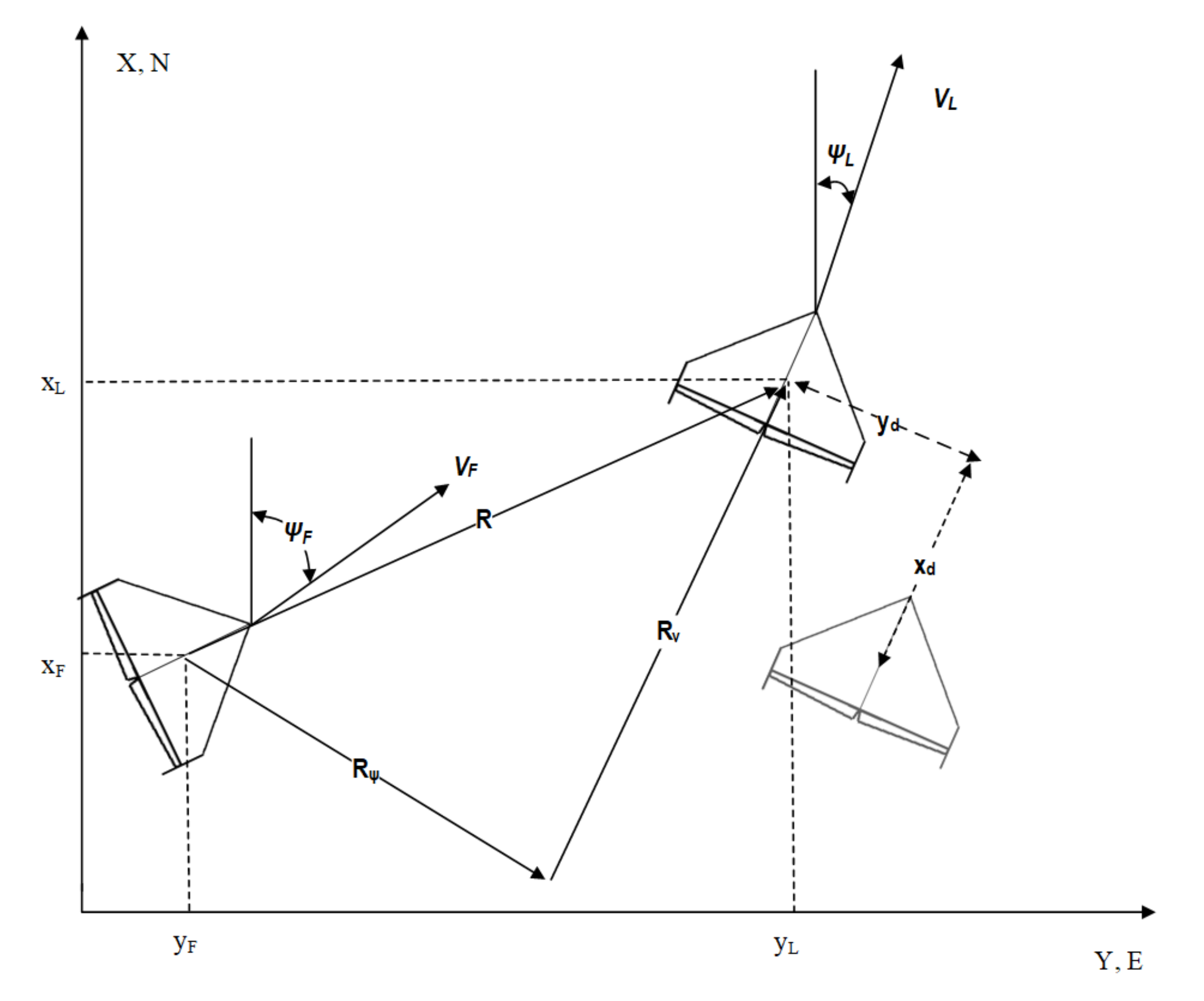
3.1. Formation Flight Geometry
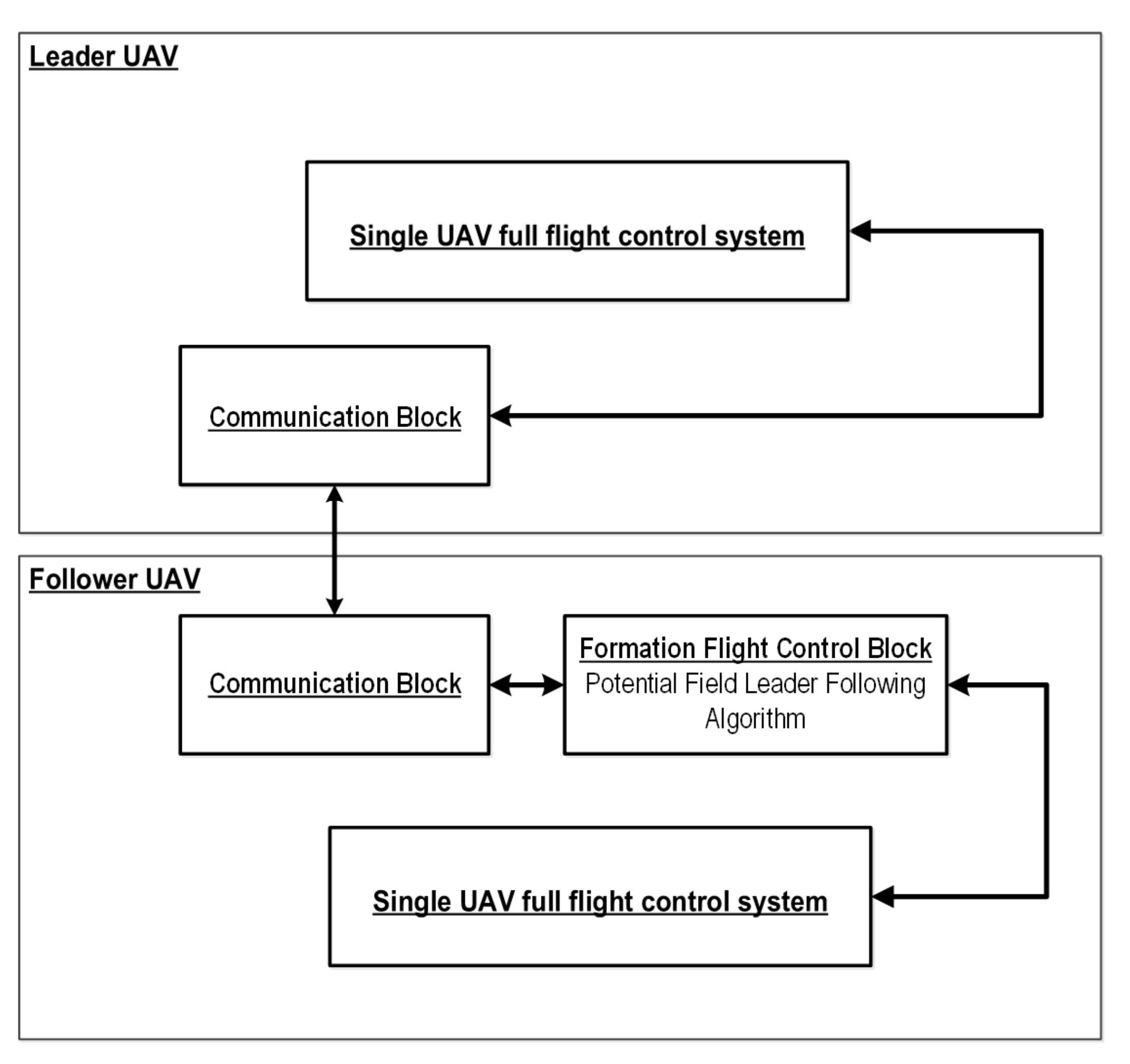
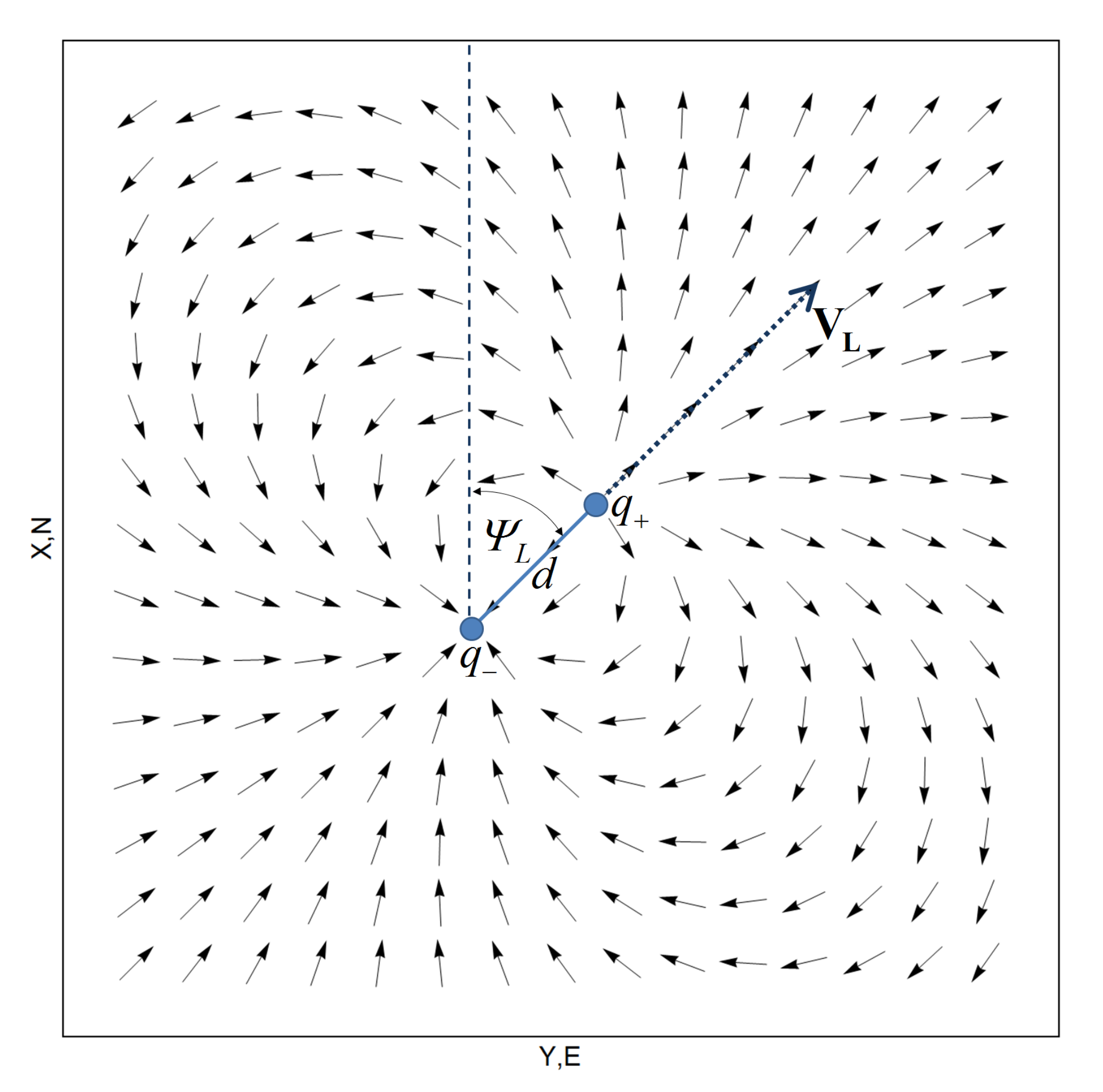
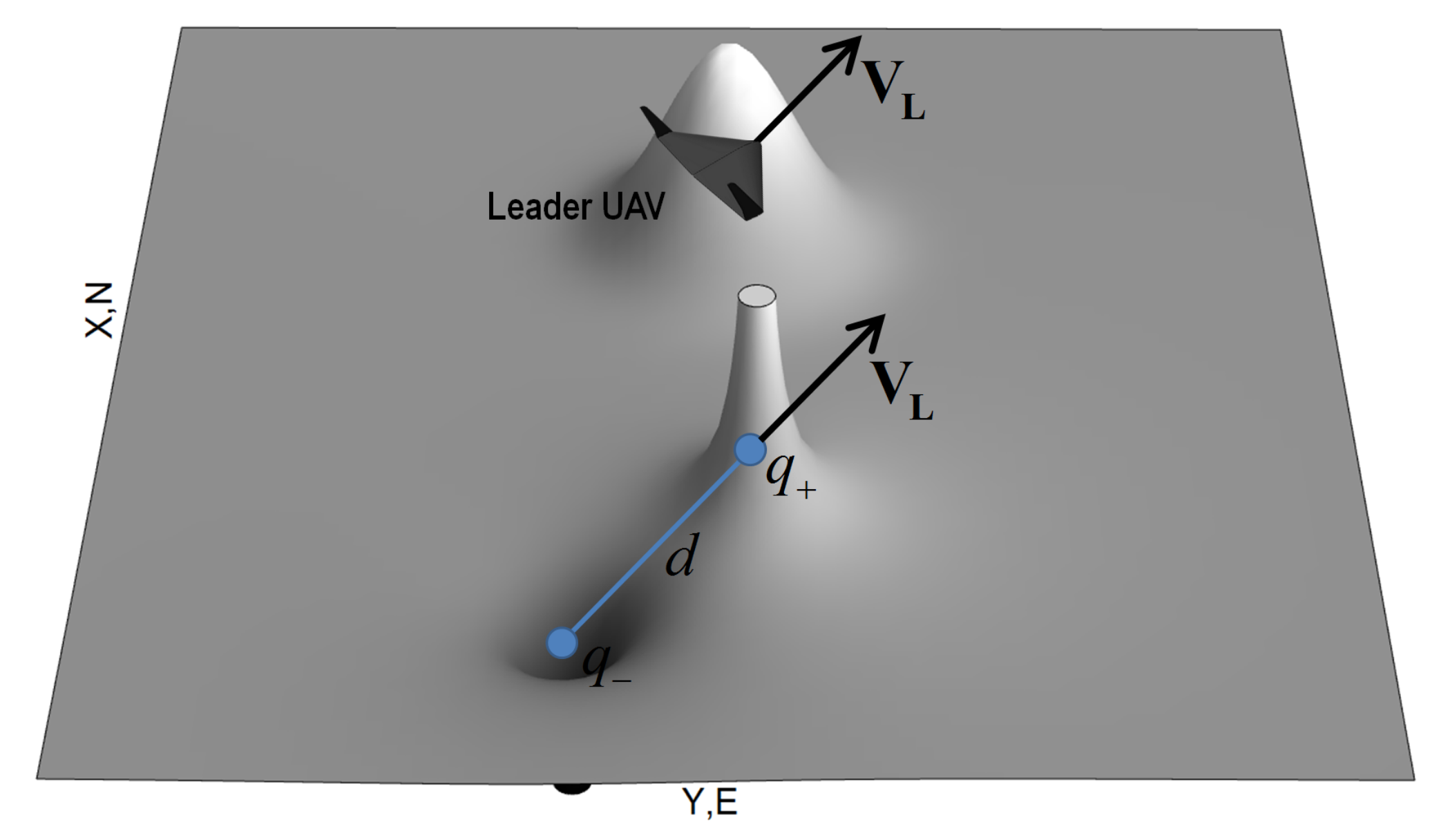
3.2. Virtual Electric Dipole Field in Leader-Follower Control Structure
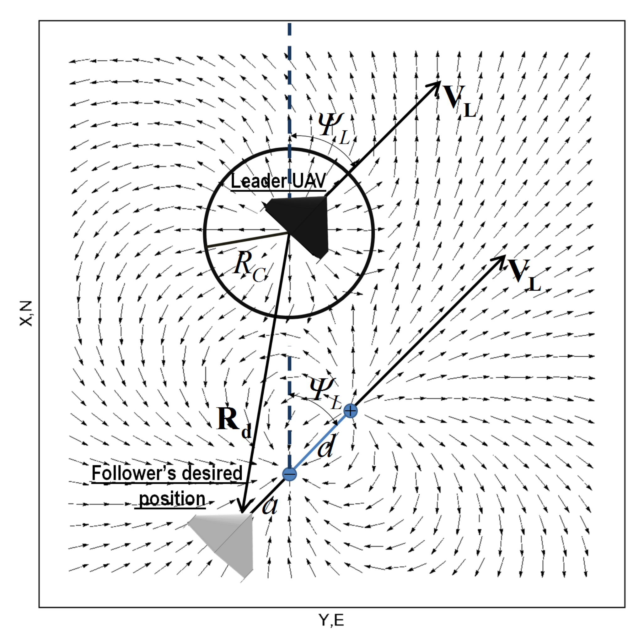
3.3. Potential Field Generation and Desired Heading Definition in Formation Flight
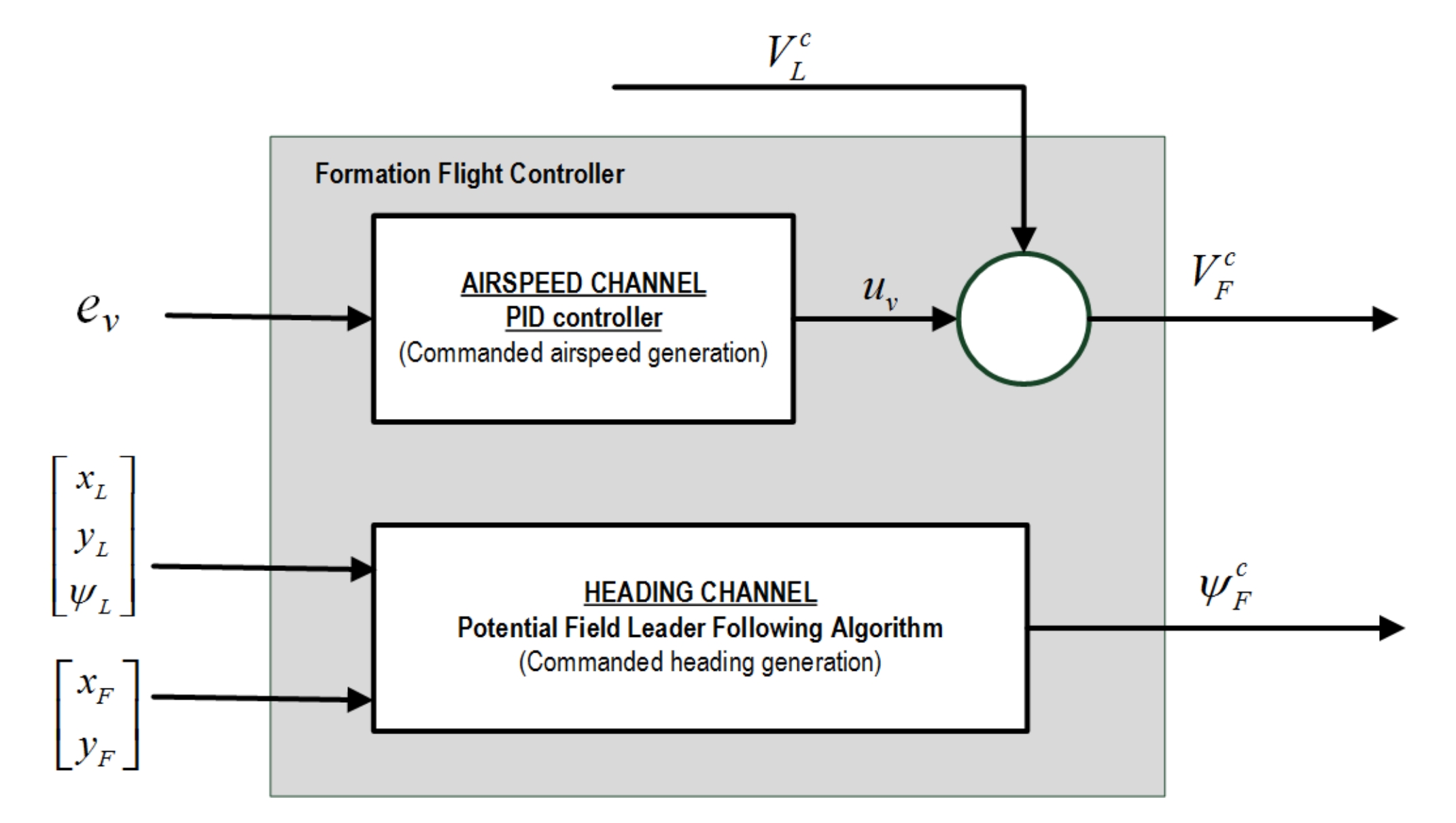
3.4. Velocity Control in Formation Flight
4. Results
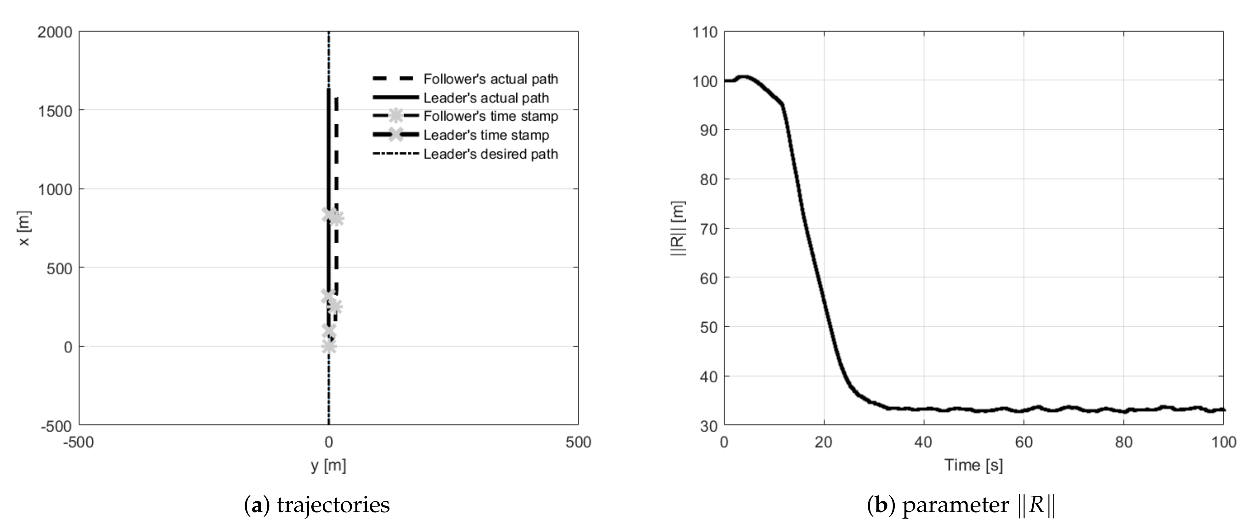
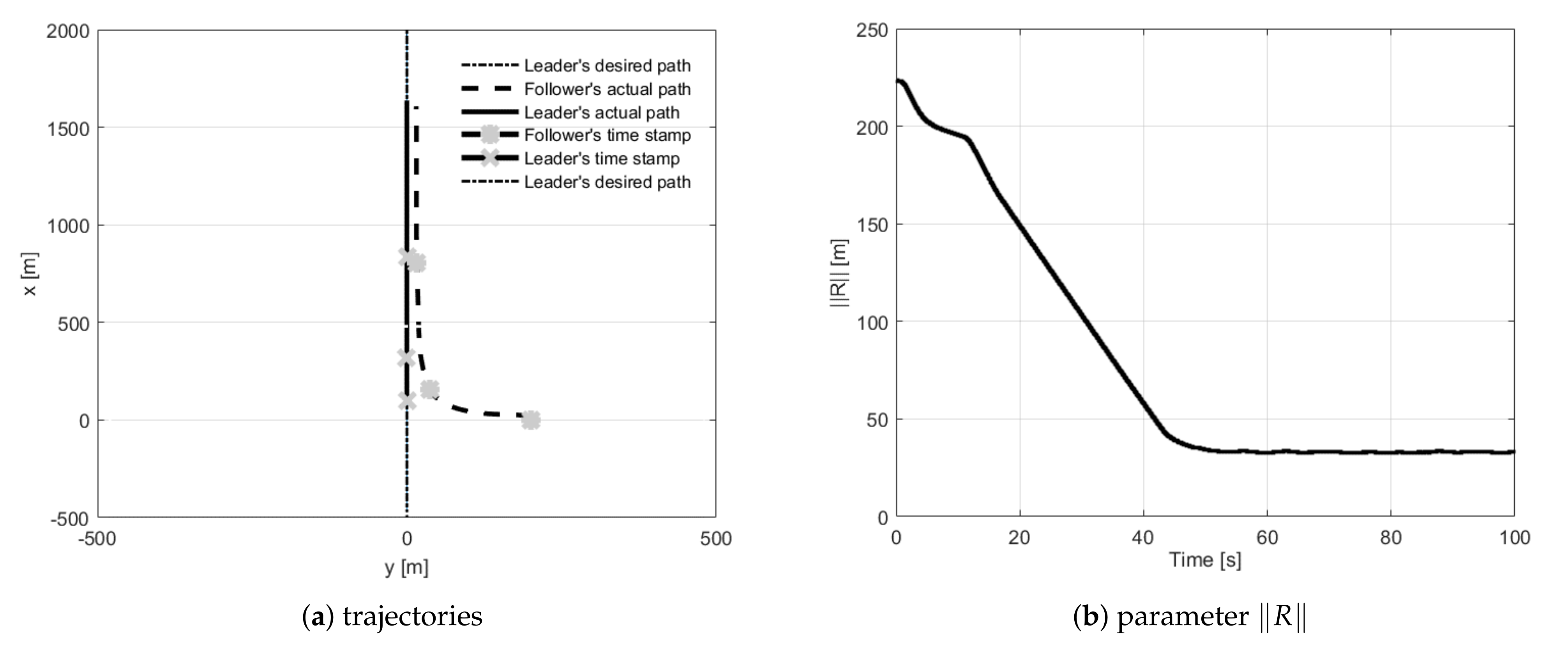
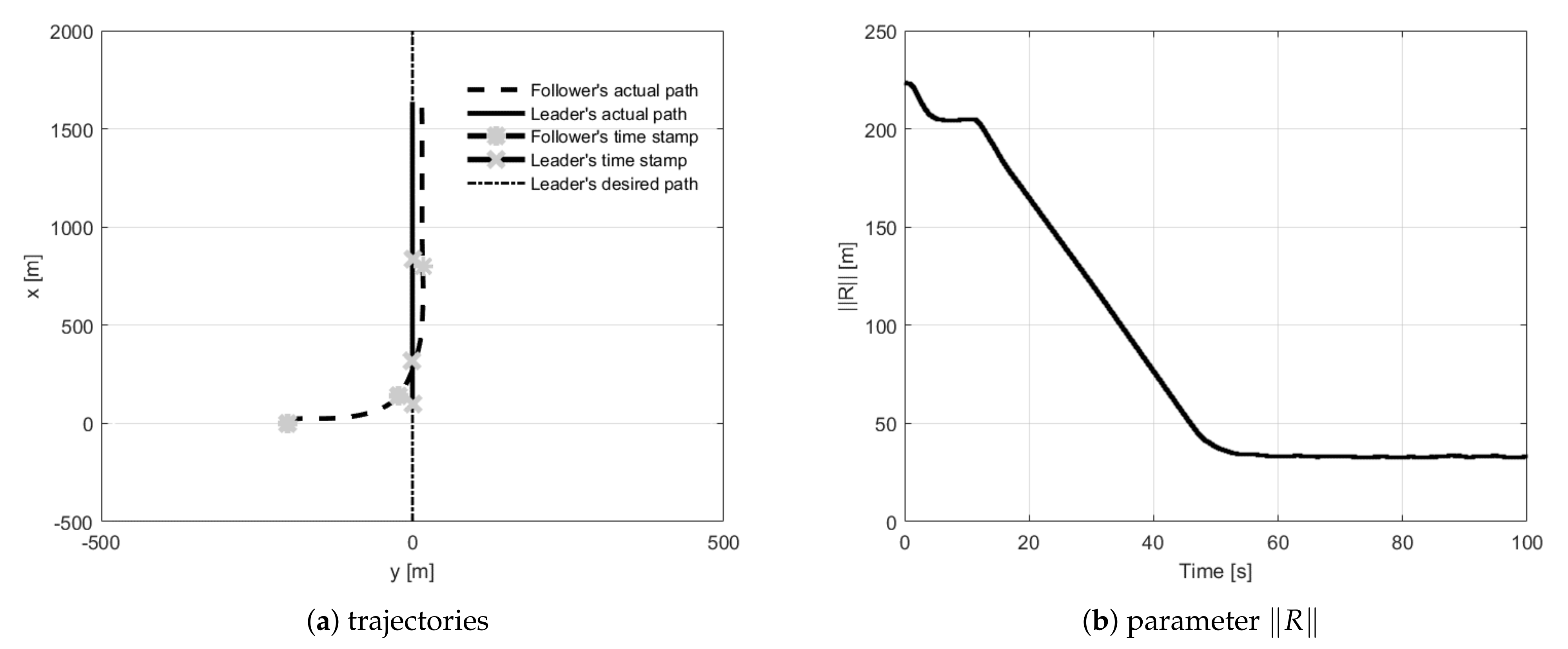
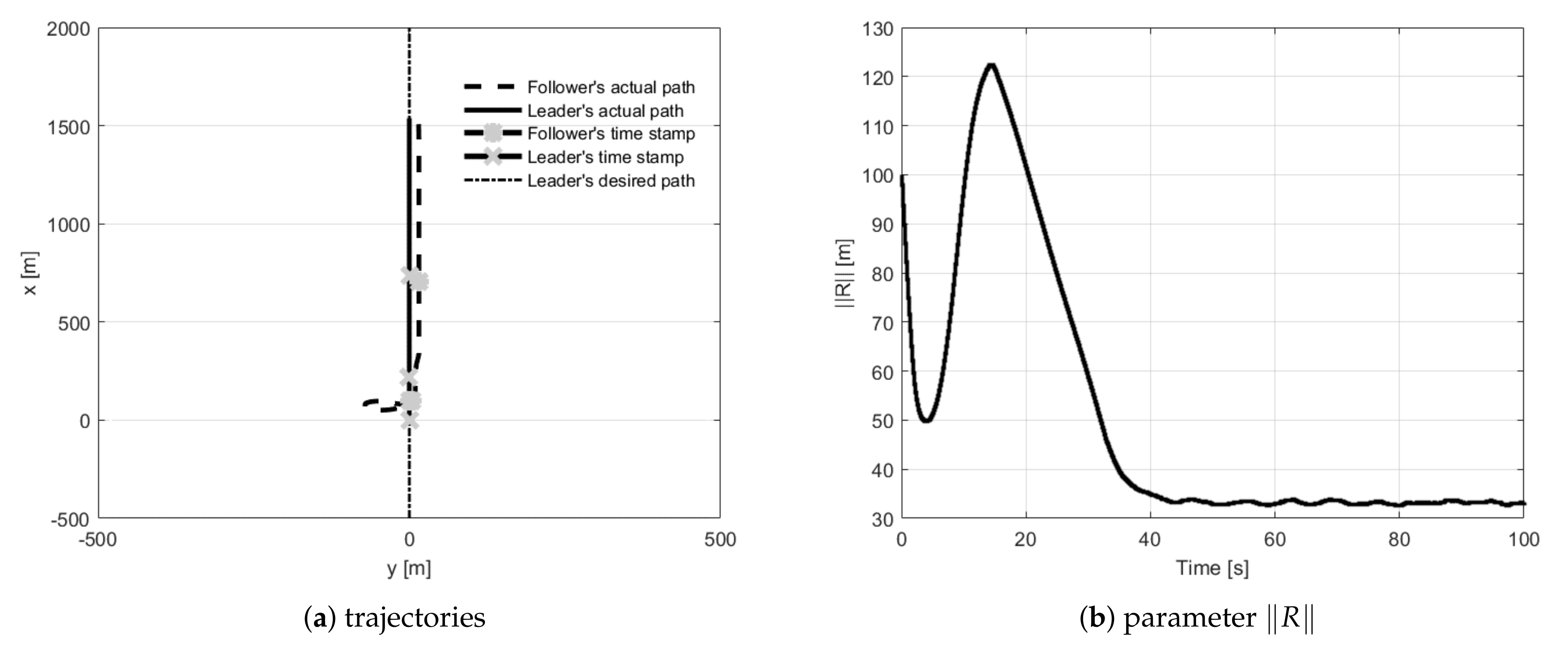
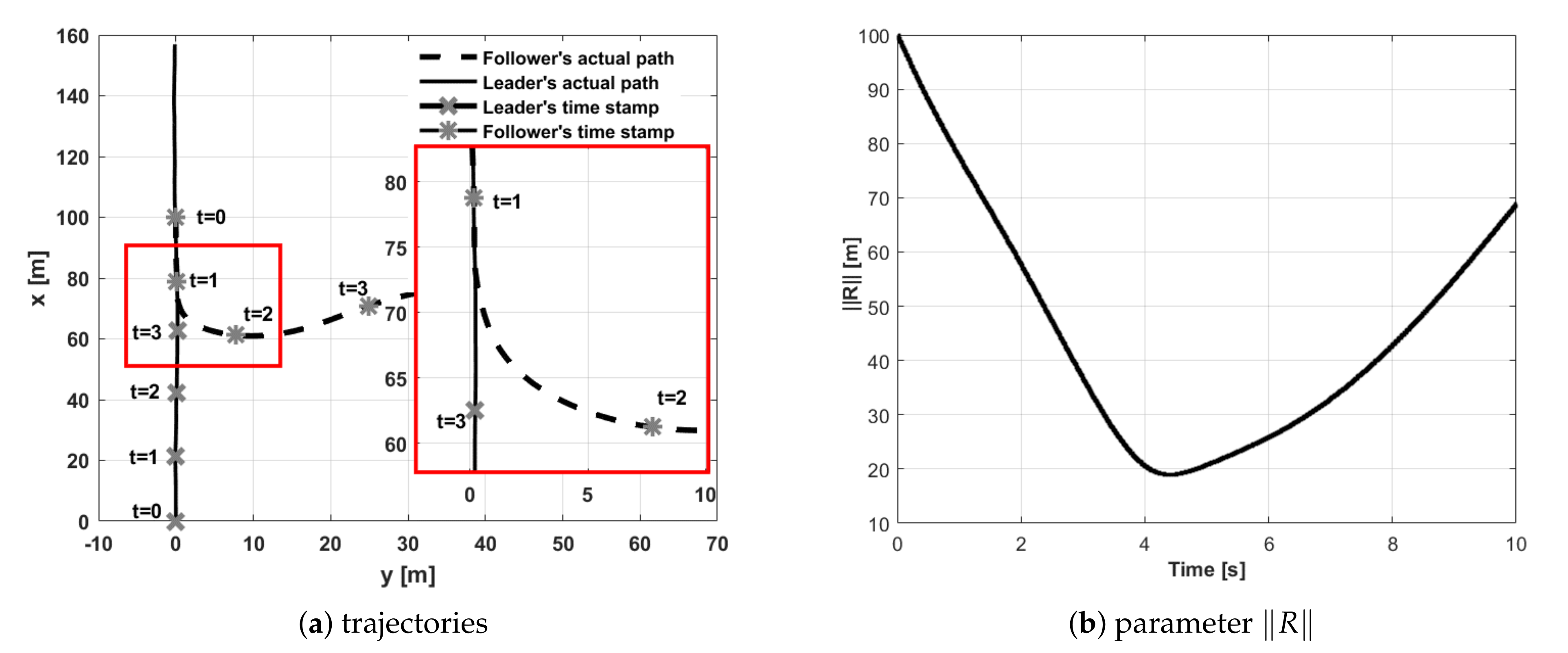
4.1. Straight Line Path Following Tests
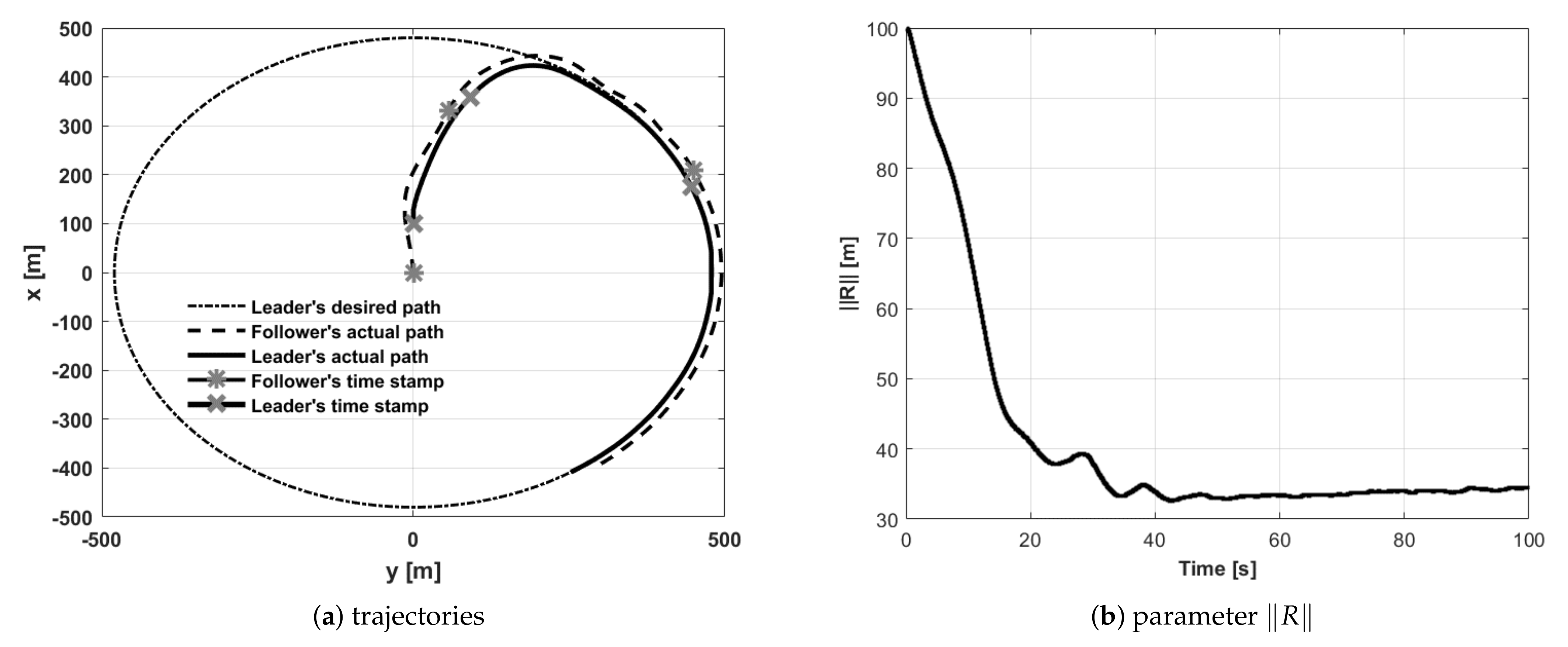
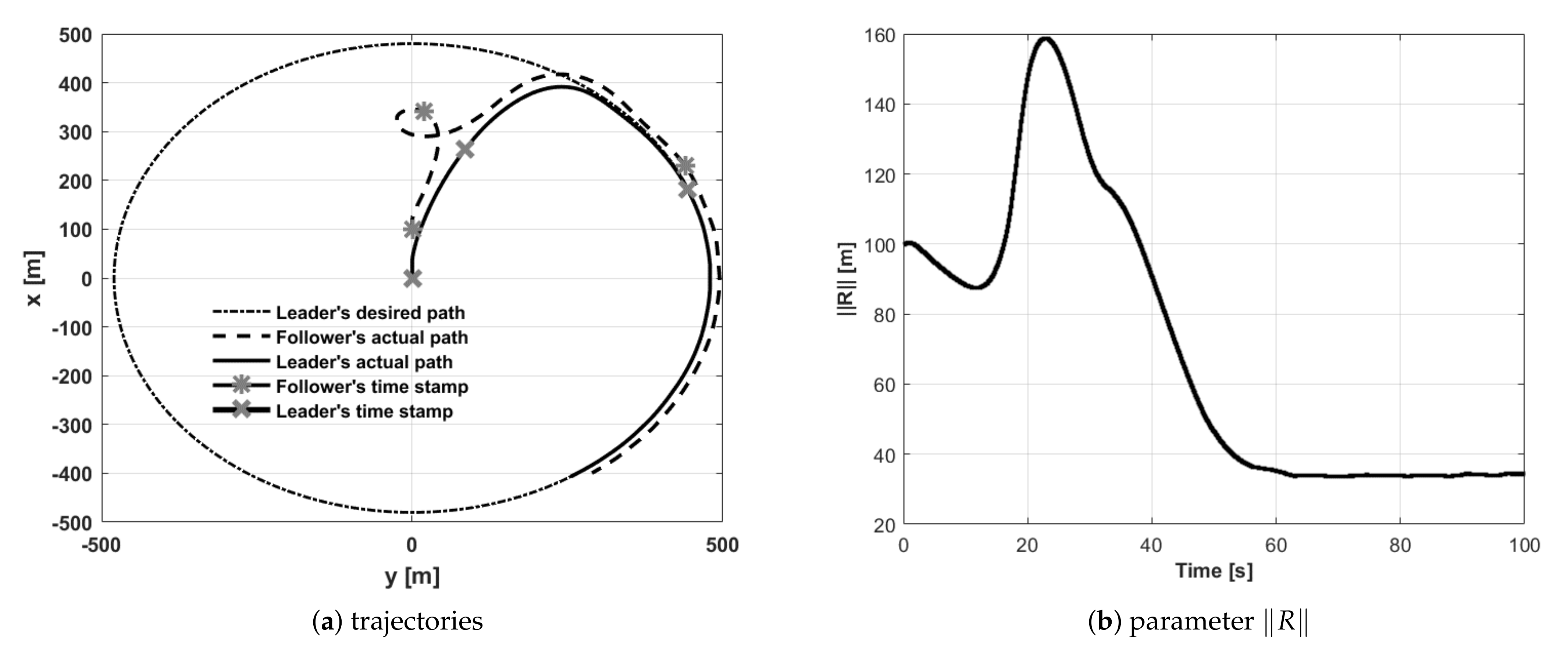
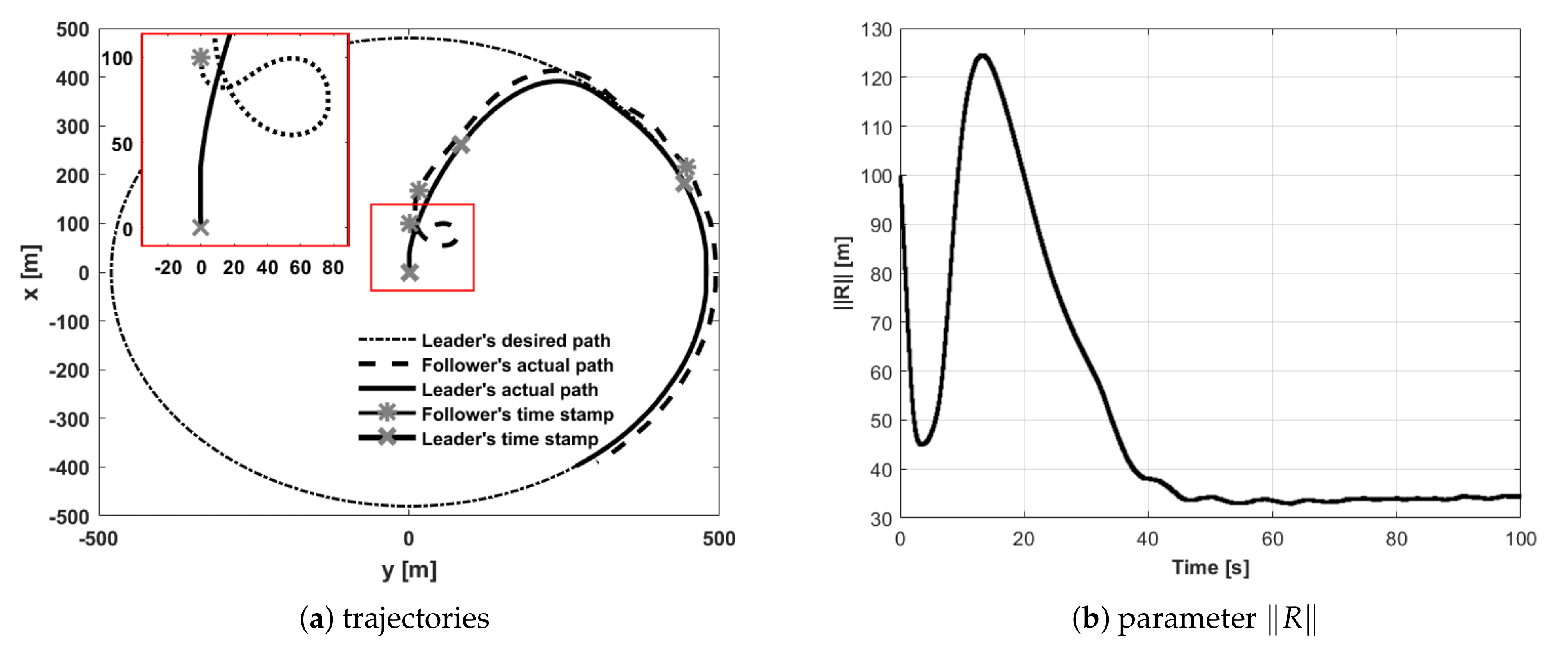
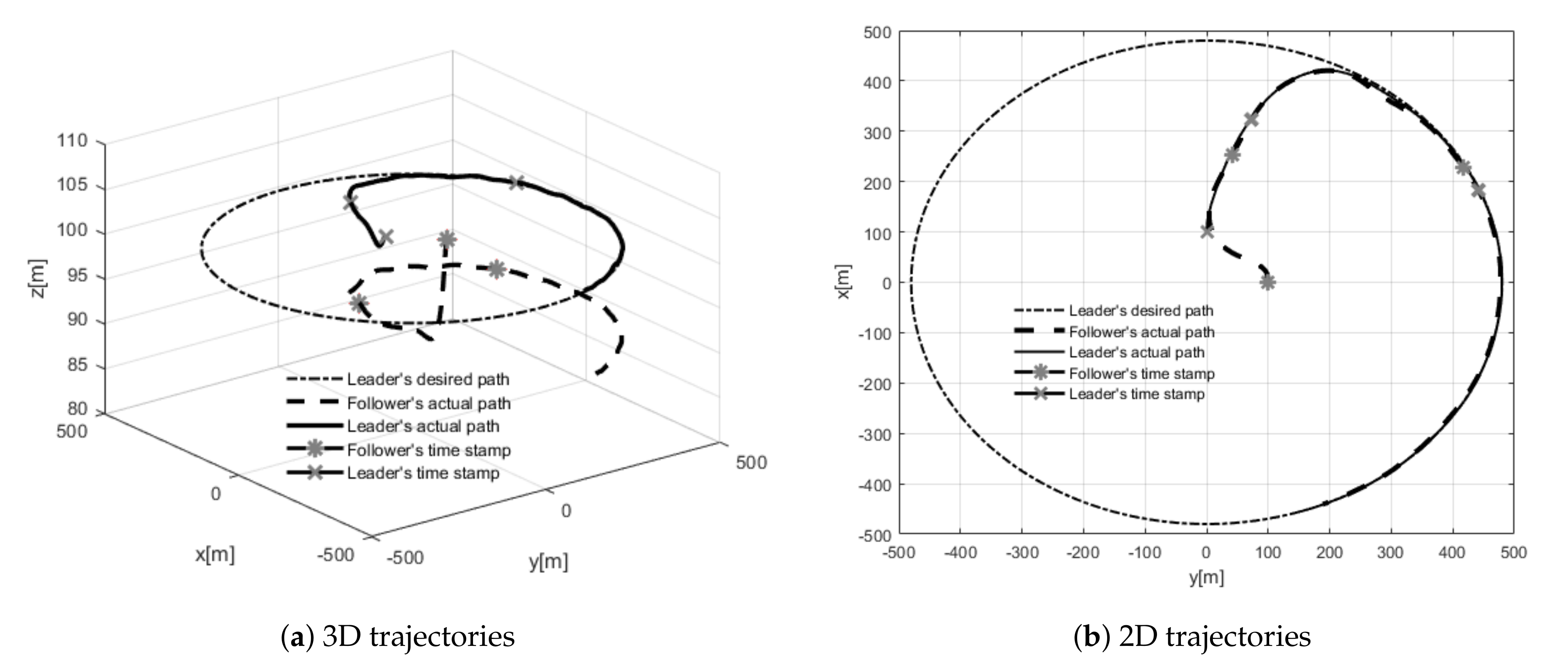
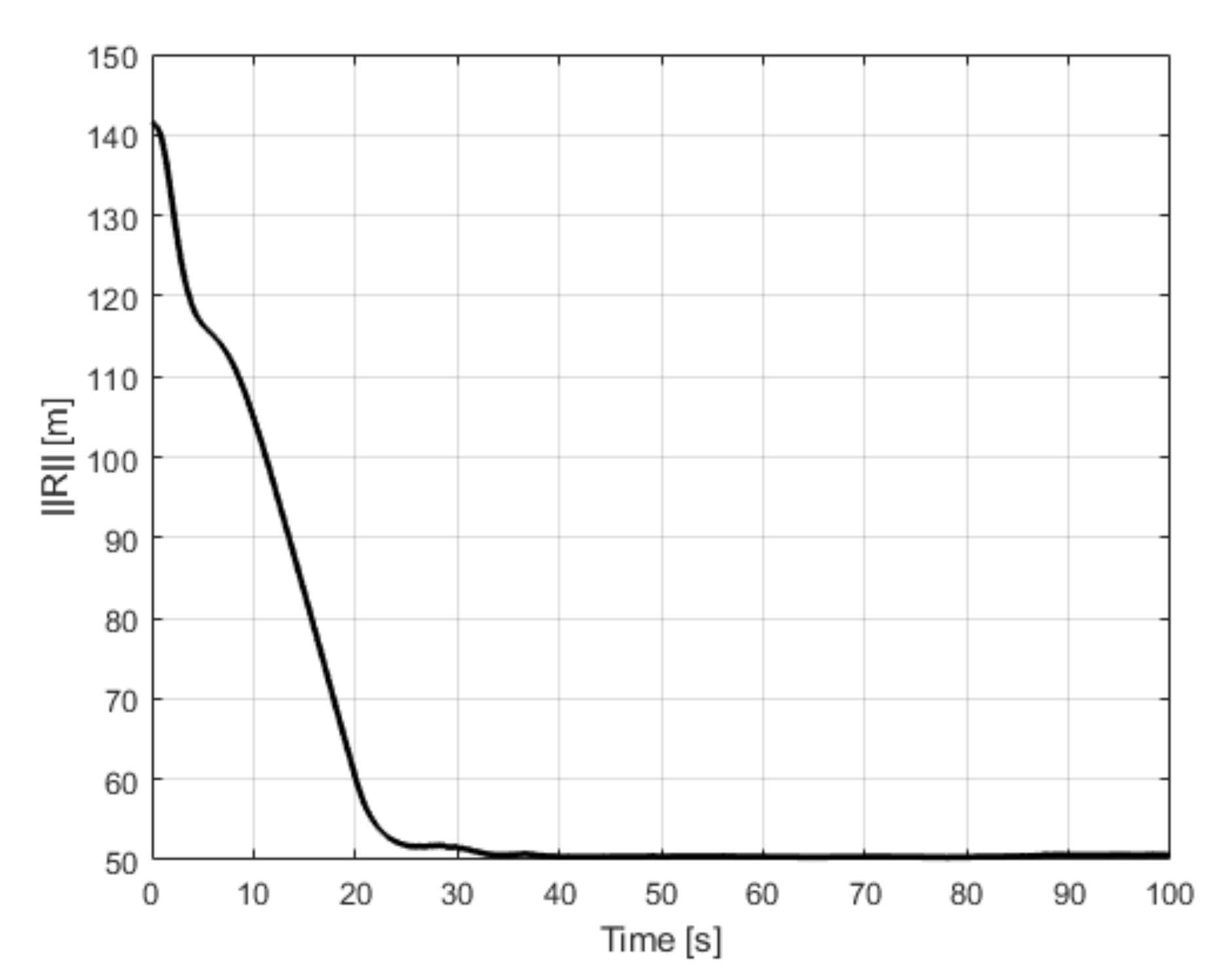
4.2. Circle Path Following Tests
5. Conclusions
Author Contributions
Funding
Institutional Review Board Statement
Informed Consent Statement
Data Availability Statement
Conflicts of Interest
References
- Gundlach, G. Designing Unmanned Aircraft Systems: A Comprehensive Approach; AIAA Education Series; American Institute of Aeronautics and Astronautics, Inc.: Reston, VA, USA, 2011. [Google Scholar]
- Nonami, K.; Kendoul, F.; Suzuki, S.; Wang, W.; Nakazawa, D. Autonomous Flying Robots, Unmanned Aerial Vehicles and Micro Aerial Vehicles; Springer: London, UK, 2010. [Google Scholar]
- Valavanis, K.P.; Vachtsevanos, G.J. Handbook of Unmanned Aerial Vehicles; Springer: Dordrecht, The Netherlands, 2015. [Google Scholar]
- Isk, A.M.; Givigi, S.N.; Fusina, G.; Beaulieu, A. Unmanned Aerial Vehicle formation flying using Linear Model Predictive Control. In Proceedings of the 2014 IEEE International Systems Conference Proceedings, San Diego, CA, USA, 5–8 October 2014; pp. 18–23. [Google Scholar]
- Cummings, M.L.; How, J.P.; Whitten, A.; Toupet, O. The Impact of Human–Automation Collaboration in Decentralized Multiple Unmanned Vehicle Control. Proc. IEEE 2012, 100, 142–149. [Google Scholar] [CrossRef]
- Khan, A.; Rinner, B.; Cavallaro, A. Multiscale observation of multiple moving targets using Micro Aerial Vehicles. In Proceedings of the International Conference on Intelligent Robots and Systems (IROS) IEEE/RSJ, Hamburg, Germany, 28 September–3 October 2015; pp. 4642–4649. [Google Scholar]
- How, J.P.; Fraser, C.; Kulling, K.C.; Ertuccelli, L.F. Increasing autonomy of UAVs. IEEE Robot. Autom. 2009, 16, 43–51. [Google Scholar] [CrossRef]
- Goddemeier, N.; Kai, D.; Wietfeld, C. Role-Based Connectivity Management with Realistic Air-to-Ground Channels for Cooperative UAVs. IEEE J. Sel. Areas Commun. 2012, 3, 951–963. [Google Scholar] [CrossRef]
- Zeng, Y.; Zhang, R.; Lim, T.J. Wireless communications with unmanned aerial vehicles: Opportunities and challenges. IEEE Commun. Mag. 2016, 54, 36–42. [Google Scholar] [CrossRef] [Green Version]
- Zhou, Y.; Cheng, N.; Lu, N.; Shen, X.S.J. Multi-UAV-Aided Networks: Aerial-Ground Cooperative Vehicular Networking Architecture. IEEE Veh. Technol. Mag. 2015, 10, 36–44. [Google Scholar] [CrossRef]
- Rady, S.; Kandil, A.A.; Badreddin, E. A hybrid localization approach for UAV in GPS denied areas. In Proceedings of the IEEE/SICE International Symposium on System Integration (SII), Kyoto, Japan, 20–22 December 2011; pp. 1269–1274. [Google Scholar]
- Romaniuk, S.; Ambroziak, L.; Gosiewski, Z.; Isto, P. Real Time Localization System with Extended Kalman Filter for Indoor Applications. In Proceedings of the 21th International Conference on Methods and Models in Automation and Robotics (MMAR), Miedzyzdroje, Poland, 29 August–1 September 2016; pp. 42–47. [Google Scholar]
- Zhou, M.; Prasad, J.V.R. Transient characteristics of a fuel cell powered UAV propulsion system. In Proceedings of the International Conference on Unmanned Aircraft Systems (ICUAS), Atlanta, GA, USA, 28–31 May 2013; pp. 114–123. [Google Scholar]
- Shiau, J.K.; Ma, D.M.; Yang, P.Y.; Wang, G.F.; Gong, J.H. Design of a Solar Power Management System for an Experimental UAV. IEEE Trans. Aerosp. Electron. Syst. 2009, 45, 1350–1360. [Google Scholar] [CrossRef]
- Kondratiuk, M.; Ambroziak, L. Concept of the Magnetic Launcher for Medium Class Unmanned Aerial Vehicles Designed on the Basis of Numerical Calculations. IEEE J. Theor. Appl. Mech. 2016, 54, 163–177. [Google Scholar] [CrossRef]
- Reck, B. First design study of an electrical catapult for unmanned air vehicles in the several hundred kilogram range. IEEE Trans. Magn. 2003, 39, 310–313. [Google Scholar] [CrossRef]
- Guruge, P.; Kocer, B.B.; Kaycan, E. A novel automatic UAV launcher design by using Bluetooth low energy integrated electromagnetic releasing system. In Proceedings of the Humanitarian Technology Conference (R10-HTC), Waterfront Hotel Cebu, Philippines, 9–12 December 2015; pp. 1–4. [Google Scholar]
- Schmitt, F.; Schulte, A. Mixed-Initiative Mission Planning Using Planning Strategy Models in Military Manned-Unmanned Teaming Missions. In Proceedings of the IEEE International Conference on Systems, Man and Cybernetics (SMC), Hong Kong, 9–12 October 2015; pp. 1391–1396. [Google Scholar]
- Olson, L.; Burns, L. A common architecture prototype for army tactical and FCS UAVS. In Proceedings of the 24th Digital Avionics Systems Conference, Washington, DC, USA, 30 October–3 November 2005; pp. 8B5.1–8B5.11. [Google Scholar]
- Giachetti, R.; Wangert, S.; Eldred, R. Interoperability Analysis Method for Mission-Oriented System of Systems Engineering. In Proceedings of the IEEE International Systems Conference (SysCon), Orlando, FL, USA, 8–11 April 2019; pp. 1–6. [Google Scholar]
- Fahlstrom, P.; Gleason, T. Introduction to UAV Systems, 4th ed.; Wiley: Chichester, UK, 2012. [Google Scholar]
- Mystkowski, A. Implementation and investigation of a robust control algorithm for an unmanned micro-aerial vehicles. Robot. Auton. Syst. 2014, 62, 1187–1196. [Google Scholar] [CrossRef]
- Kownacki, C. Design of an adaptive Kalman filter to eliminate measurement faults of a laser rangefinder used in the UAV system. Aerosp. Sci. Technol. 2015, 41, 81–89. [Google Scholar] [CrossRef]
- Zhiteckii, L.S.; Pilchevsky, A.Y.; Kravchenko, A.O.; Bykov, B.V. Modern control theory for designing lateral autopilot systems of UAV. In Proceedings of the IEEE International Conference on Actual Problems of Unmanned Aerial Vehicles Developments (APUAVD), Kyiv, UKraine, 13–15 October 2015; pp. 160–164. [Google Scholar]
- Guerrero, J.A.; Lozano, R. Flight Formation Control; Wiley-ISTE: Hoboken, NJ, USA, 2012. [Google Scholar]
- Rabbath, C.A.; Lechevin, N. Safety and Reliability in Cooperating Unmanned Aerial Systems; World Scientific Publishing Company: Singapore, 2010. [Google Scholar]
- Gosiewski, Z.; Ambroziak, L. Formation Flight Control Scheme for Unmanned Aerial Vehicles. Lect. Notes Control Inf. Sci. 2012, 422, 331–340. [Google Scholar]
- Kownacki, C.; Ambroziak, L. Flight control of a formation of fixed-wing UAVs based on the idea of flexible structure. In Proceedings of the 12th International Conference Mechatronic Systems and Materials MSM 2016—Intelligent Technical Systems, Bialystok, Poland, 3–8 July 2016. [Google Scholar]
- Giulietti, F.; Innocenti, M.; Innocenti, M.; Pollini, L. Dynamic and control issues of formation flight. Aerosp. Sci. Technol. 2005, 9, 65–71. [Google Scholar] [CrossRef]
- Giulietti, F.; Pollini, L.; Innocenti, M. Autonomous Formation Flight. IEEE Control Syst. Mag. 2000, 20, 34–44. [Google Scholar]
- Johnson, E.N.; Calise, A.J.; Sattigeri, R.; Watanable, Y.; Madyastha, V. Approaches to vision-based formation control. In Proceedings of the 43rd IEEE Conference on Decision and Control CDC, Paradise Island, The Bahamas, 14–17 December 2004; pp. 1643–1648. [Google Scholar]
- Lin, F.; Peng, K.; Dong, X.; Zhao, S.; Chen, B.M. Vision-based Formation for UAVs. In Proceedings of the 11th IEEE International Conference on Control & Automation (ICCA), Taichung, Taiwan, 18–20 June 2014; pp. 1375–1380. [Google Scholar]
- Dehghani, M.A.; Menhaj, M.B. Integral sliding mode formation control of fixed-wing unmanned aircraft using seeker as a relative measurement system. Aerosp. Sci. Technol. 2016, 48, 318–327. [Google Scholar] [CrossRef]
- Lvlong, H.; Peng, B.; Xiaolong, L.; Jiaqiang, Z.; Weijia, W. Feedback formation control of UAV swarm with multiple implicit leaders. Aerosp. Sci. Technol. 2018, 72, 327–334. [Google Scholar]
- Jianhua, W.; Liang, H.; Xiwang, D.; Qingdong, L.; Zhang, R. Distributed sliding mode control for time-varying formation tracking of multi-UAV system with a dynamic leader. Aerosp. Sci. Technol. 2021, 111, 106549. [Google Scholar]
- Li, N.H.M.; Liu, H.H.T. Formation UAV flight control using virtual structure and motion synchronization. In Proceedings of the American Control Conference, Seattle, WA, USA, 11–13 June 2008; pp. 1782–1787. [Google Scholar]
- Kownacki, C.; Ołdziej, D. Fixed-wing UAVs Flock Control through Cohesion and Repulsion Behaviors Combined with a Leadership. Int. J. Adv. Robot. Syst. 2016, 13, 36. [Google Scholar] [CrossRef] [Green Version]
- Muslimov, T.R.; Munasypov, R.A. DConsensus-based cooperative control of parallel fixed-wing UAV formations via adaptive backstepping. Aerosp. Sci. Technol. 2021, 109, 106416. [Google Scholar] [CrossRef]
- Ziquan, Y.; Youmin, Z.; Bin, J.; Xiang, Y.; Jun, F.; Ying, J.; Tianyou, C. Distributed adaptive fault-tolerant close formation flight control of multiple trailing fixed-wing UAVs. ISA Trans. 2020, 106, 181–199. [Google Scholar]
- Hao, L.; Qingyao, M.; Fachun, P.; Frank, L.L. Heterogeneous formation control of multiple UAVs with limited-input leader via reinforcement learning. Neurocomputing 2020, 412, 63–71. [Google Scholar]
- Buzogany, L.E.; Pachter, M.; D’azzo, J.J. Automated control of aircraft in formation flight. In Proceedings of the AIAA Guidance, Navigation and Control Conference, Monterey, CA, USA, 9–11 August 1993; pp. 1349–1370. [Google Scholar]
- Hall, J.K.; Pachter, M. Formation maneuvers in three dimensions. In Proceedings of the 39th IEEE Conference on Decision and Control, Sydney, NSW, Australia, 12–15 December 2000; pp. 364–369. [Google Scholar]
- Pachter, M.; D’azzo, J.; Dargan, J.L. Automatic formation flight control. J. Guid. Control. Dyn. 1994, 17, 1380–1383. [Google Scholar] [CrossRef]
- Cheng, Z.; Necsulescu, D.S.; Kim, B.; Sasiadek, J.Z. Nonlinear Control for UAV Formation Flying. In Proceedings of the 17th World Congress The International Federation of Automatic Control, Seoul, Korea, 6–11 July 2008; pp. 791–796. [Google Scholar]
- Kim, D.M.; Nam, S.; Suk, J. A modified nonlinear guidance logic for a leader-follower formation flight of two UAVs. In Proceedings of the ICCAS-SICE Conference, Fukuoka City, Japan, 18–21 August 2009; pp. 5734–5739. [Google Scholar]
- Ambroziak, L.; Gosiewski, Z. Two stage switching control for autonomous formation flight of unmanned aerial vehicles. Aerosp. Sci. Technol. 2015, 46, 221–226. [Google Scholar] [CrossRef]
- McCammish, S.; Pachter, M.; D’azzo, J.J.; Reyna, V. Optimal Formation Flight Control. In Proceedings of the AIAA Guidance, Navigation and Control Conference, San Diego, CA, USA, 29–31 July 1996. [Google Scholar]
- Du, M.; Yamashita, Y. Optimal Control of Formation Flight Based on MLD Systems. In Proceedings of the IEEE International Conference on Control Applications, Singapore, 1–3 October 2007; pp. 904–909. [Google Scholar]
- Boskowic, J.D.; Sun, Z.; Song, Y.D. An adaptive reconfigurable formation flight control design. In Proceedings of the 2003 American Control Conference, Denver, CO, USA, 4–6 June 2003; pp. 284–289. [Google Scholar]
- Schumacher, C.J.; Kumar, R. Adaptive control of UAVs in close-coupled formation flight. In Proceedings of the American Control Conference, Denver, CO, USA, 4–6 June 2003; pp. 849–853. [Google Scholar]
- Shin, J.; Kim, H.J. Nonlinear Model Predictive Formation Flight. IEEE Trans. Syst. Man Cybern. Part A Syst. Humans 2009, 39, 1116–1125. [Google Scholar] [CrossRef]
- Li, B.; Liao, X.H.; Sun, Z.; Li, Y.; Song, Y.D. Robust Autopilot for Close Formation Flight of Multi-UAVs. In Proceedings of the 2006 Thirty-Eighth Southeastern Symposium on System Theory, Cookeville, TN, USA, 5–7 March 2006; pp. 258–262. [Google Scholar]
- Raffard, R.L.; Tomlin, C.J.; Boyd, S.P. Distributed optimization for cooperative agents: Application to formation flight. In Proceedings of the 43rd IEEE Conference on Decision and Control CDC, Paradise Island, Bahamas, 14–17 December 2004; pp. 2453–2459. [Google Scholar]
- Kuwata, Y.; How, J.P. Cooperative Distributed Robust Trajectory Optimization Using Receding Horizon MILP. IEEE Trans. Control Syst. Technol. 2011, 19, 423–431. [Google Scholar] [CrossRef]
- Radmanesh, M.; Kumar, M. Flight formation of UAVs in presence of moving obstacles using fast-dynamic mixed integer linear programming. Aerosp. Sci. Technol. 2016, 50, 149–160. [Google Scholar] [CrossRef] [Green Version]
- Chen, Y.; Yu, J.; Su, X.; Luo, G. Path Planning for Multi-UAV Formation. J. Intell. Robot. Syst. 2015, 77, 229–246. [Google Scholar] [CrossRef]
- Suzuki, M.; Uchiyama, K.; Bennet, D.; Macinnes, C. Three-Dimensional Formation Flying Using Bifurcating Potential Fields. In Proceedings of the AIAA Guidance, Navigation, and Control Conference, Toronto, ON, Canada, 8–11 August 2009; pp. 1–11. [Google Scholar]
- Nagao, Y.; Uchiyama, K. Formation Flight of Fixed- Wing UAVS Using Artificial Potential Field. In Proceedings of the 29th Congress of the International Council of the Aeronautical Sciences, St. Petersburg, Russia, 7–12 September 2014; pp. 1–8. [Google Scholar]
- Kokume, M.; Uchiyama, K. Guidance Law Based on Bifurcating Velocity Field for Formation Flight. In Proceedings of the AIAA Guidance, Navigation, and Control Conference, Guidance, Navigation, Toronto, ON, Canada, 2–5 August 2010; pp. 1–10. [Google Scholar]
- Paul, T.; Krogstad, T.R.; Gravdhal, J.T. Modelling of UAV Flight Using 3D potential Field. Simul. Model. Pract. Theory 2008, 16, 1453–1462. [Google Scholar] [CrossRef]
- Tahk, M.J.; Park, C.S.; Ryoo, C.K. Line-of-sight guidance laws for formation flight. J. Guid. Control. Dyn. 2005, 28, 708–716. [Google Scholar] [CrossRef]
- Betser, A.; Vela, P.A.; Pryor, G. Tannenbaum, Flying in formation using a pursuit guidance algorithm. In Proceedings of the American Control Conference, Portland, OR, USA, 8–10 June 2005; pp. 5085–5090. [Google Scholar]
- Available online: www.topmodelcz.cz (accessed on 20 April 2021).
- Beard, R.W.; McLain, T.W. Small Unmanned Aircraft, Theory and Practice; Princeton University Press: Princeton, NJ, USA, 2012. [Google Scholar]
- Roskam, J. Airplane Flight Dynamics and Automatic Flight Controls, Parts I & II; DAR Corporation: Lawrence, KS, USA, 2012. [Google Scholar]
- Stevens, B.L.; Lewis, F.L. Aircraft Control and Simulation, 2nd ed.; John Wiley & Sons: Hoboken, NJ, USA, 2003. [Google Scholar]
- Available online: https://www.darcorp.com/advanced-aircraft-analysis-software/ (accessed on 20 April 2012).
- Available online: http://tornado.redhammer.se (accessed on 20 April 2012).
- Ambroziak, L.; Gosiewski, Z.; Kondratiuk, M. Aerodynamics Characteristics Identification of Micro Air Vehicle. Trans. Inst. Aviat. 2011, 216, 17–29. (In Polish) [Google Scholar]
- Nise, N.S. Control Systems Engineering, 8th ed.; John Wiley & Sons: Hoboken, NJ, USA, 2019. [Google Scholar]
- Rauw, M. FDC 1.2—A Simulink Toolbox for Flight Dynamics and Control Analysis, 2nd ed.; 2001. Available online: https://www.semanticscholar.org/paper/FDC-1.2-A-Simulink-Toolbox-for-Flight-Dynamics-and-Rauw/dfbc4526f57f83e97c030b527fd0b6dfc2afdeaf (accessed on 30 June 2021).
- Available online: https://www.mathworks.com/help/aeroblks/ (accessed on 20 April 2012).
- Available online: https://www.micropilot.com/ (accessed on 20 April 2012).
- Available online: https://www.lockheedmartin.com/content/dam/lockheed-martin/rms/photo/procerus/Kestrel-Flight-Systems-brochure.pdf. (accessed on 20 April 2012).
- Rankin, J. GPS and differential GPS: An error model for sensor simulation. In Proceedings of the Position, Location and Navigation Symposium, Las Vegas, NV, USA, 10–15 April 1994; pp. 260–266. [Google Scholar]
- Khatib, O. Real-time obstacle avoidance for manipulators and mobile robots. Int. J. Robot. Res. 1986, 17, 90–98. [Google Scholar] [CrossRef]
- AL-Sultan, K.; Aliyu, M. A new potential field-based algorithm for path planning. J. Intell. Robot. Syst. 1996, 17, 265–282. [Google Scholar] [CrossRef]
- Xiao, B.; Yu, L.; Li, S.; Chen, R. Research of escaping local minima strategy for artificial potential field. J. Syst. Simul. 2007, 19, 4495–4503. [Google Scholar]
- Montiel, O.; Orozco-Rosas, U.; Sepulvda, R. Path planning for mobile robots using Bacterial Potential Field for avoiding static and dynamic obstacles. Expert Syst. Appl. 2015, 42, 5177–5191. [Google Scholar] [CrossRef]
- Langelaan, J.W.; Alley, N.; Neidhoefer, J. Wind field estimation for small unmanned aerial vehicles. J. Guid. Control. Dyn. 2011, 34, 1016–1030. [Google Scholar] [CrossRef]


| Moment of Inertia | Value |
|---|---|
| I | 0.091108 [kgm] |
| I | 0.076144 [kgm] |
| I | 0.165955 [kgm] |
| I | 0.0011547 [kgm] |
| 0.14635 | 0.00293 | −0.030586 | 2.8074 | 0.08759 | −0.59632 |
| 4.0992 | 0.12967 | −1.6137 | 1.05 | 0.0338 | −0.61558 |
| −6.6478 × 10 | 4.3476 × 10 | 6.855 × 10 | −0.022517 | −0.043166 |
| −0.0608 | 0.1144 | −0.13669 | 0.0293 | −0.14037 |
| 0.026176 | −0.038383 | −2.8334 × 10 | 1.8034 × 10 | −9.3649 × 10 |
| Test Number | Leader Initial Positions () | Follower Initial Positions () | Desired Distances during Formation Flight | Initial Headings | ||||||
|---|---|---|---|---|---|---|---|---|---|---|
| [m] | [m] | [m] | [m] | [m] | [m] | [m] | [m] | [rad] | [rad] | |
| 1 | 100 | 0 | 100 | 0 | 0 | 100 | −30 | −15 | 0 | 0 |
| 2 | 100 | 0 | 100 | 0 | 200 | 100 | −30 | −15 | 0 | 0 |
| 3 | 100 | 0 | 100 | 0 | −200 | 100 | −30 | −15 | 0 | 0 |
| 4 | 0 | 0 | 100 | 100 | 0 | 100 | −30 | −15 | 0 | |
| Test Number | Leader Initial Positions () | Follower Initial Positions () | Desired Distances during Formation Flight | Initial Headings | |||||||
|---|---|---|---|---|---|---|---|---|---|---|---|
| [m] | [m] | [m] | [m] | [m] | [m] | [m] | [m] | [m] | [rad] | [rad] | |
| 5 | 100 | 0 | 100 | 0 | 0 | 100 | −30 | −15 | 0 | 0 | 0 |
| 6 | 0 | 0 | 100 | 100 | 0 | 100 | −30 | −15 | 0 | 0 | 0 |
| 7 | 0 | 0 | 100 | 100 | 0 | 100 | −30 | −15 | 0 | 0 | |
| 8 | 100 | 0 | 100 | 0 | 0 | 100 | −50 | 0 | −10 | 0 | 0 |
| Test Number | RMSE [m] | RRMSE [%] |
|---|---|---|
| 1 | 0.2238 | 0.6672 |
| 2 | 0.2339 | 0.6974 |
| 3 | 0.2376 | 0.7084 |
| 4 | 0.2289 | 0.6824 |
| 5 | 0.2790 | 0.8318 |
| 6 | 0.2641 | 0.7874 |
| 7 | 0.2800 | 0.8348 |
| Communication Time Delay [sec] | RMSE [m] | RRMSE [%] |
|---|---|---|
| 0.1 | 1.1602 | 3.4590 |
| 0.5 | 1.2438 | 3.7083 |
| 1.0 | 1.3407 | 3.9972 |
| 1.5 | 1.4736 | 4.3934 |
| 2.0 | 1.5844 | 4.7238 |
Publisher’s Note: MDPI stays neutral with regard to jurisdictional claims in published maps and institutional affiliations. |
© 2021 by the authors. Licensee MDPI, Basel, Switzerland. This article is an open access article distributed under the terms and conditions of the Creative Commons Attribution (CC BY) license (https://creativecommons.org/licenses/by/4.0/).
Share and Cite
Ambroziak, L.; Ciężkowski, M. Virtual Electric Dipole Field Applied to Autonomous Formation Flight Control of Unmanned Aerial Vehicles. Sensors 2021, 21, 4540. https://doi.org/10.3390/s21134540
Ambroziak L, Ciężkowski M. Virtual Electric Dipole Field Applied to Autonomous Formation Flight Control of Unmanned Aerial Vehicles. Sensors. 2021; 21(13):4540. https://doi.org/10.3390/s21134540
Chicago/Turabian StyleAmbroziak, Leszek, and Maciej Ciężkowski. 2021. "Virtual Electric Dipole Field Applied to Autonomous Formation Flight Control of Unmanned Aerial Vehicles" Sensors 21, no. 13: 4540. https://doi.org/10.3390/s21134540