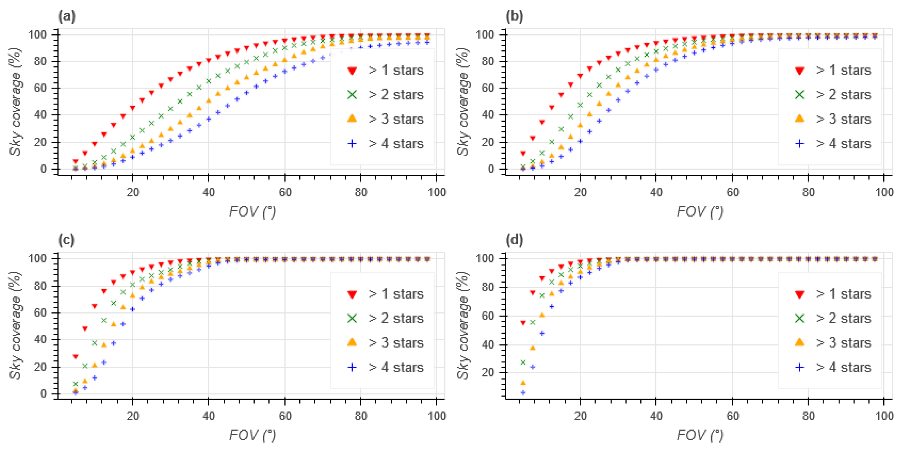
Figure 1.
Sky coverage vs FOV for given maximum apparent magnitude (a) mag < 3 (b) mag < 4 (c) mag < 5 (d) mag < 6.
Figure 1.
Sky coverage vs FOV for given maximum apparent magnitude (a) mag < 3 (b) mag < 4 (c) mag < 5 (d) mag < 6.
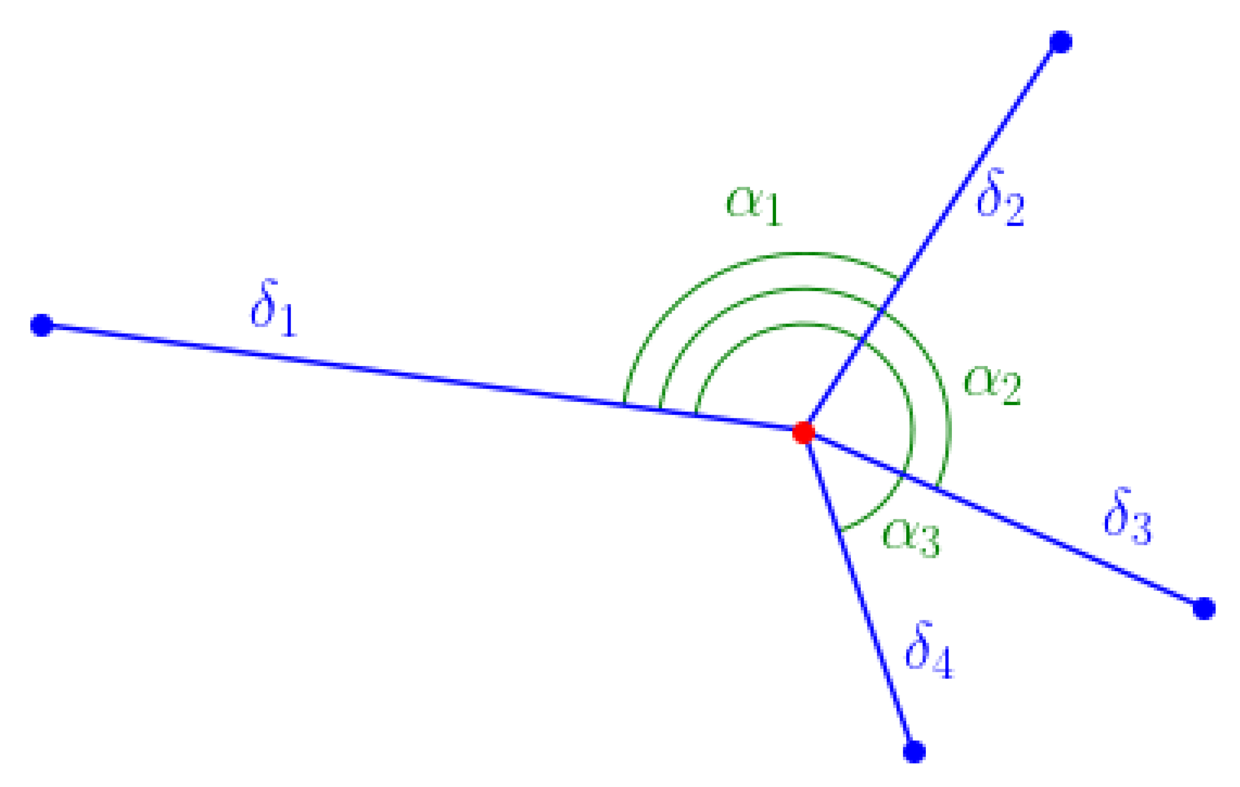
Figure 2.
Feature descriptor of four stars.
Figure 2.
Feature descriptor of four stars.
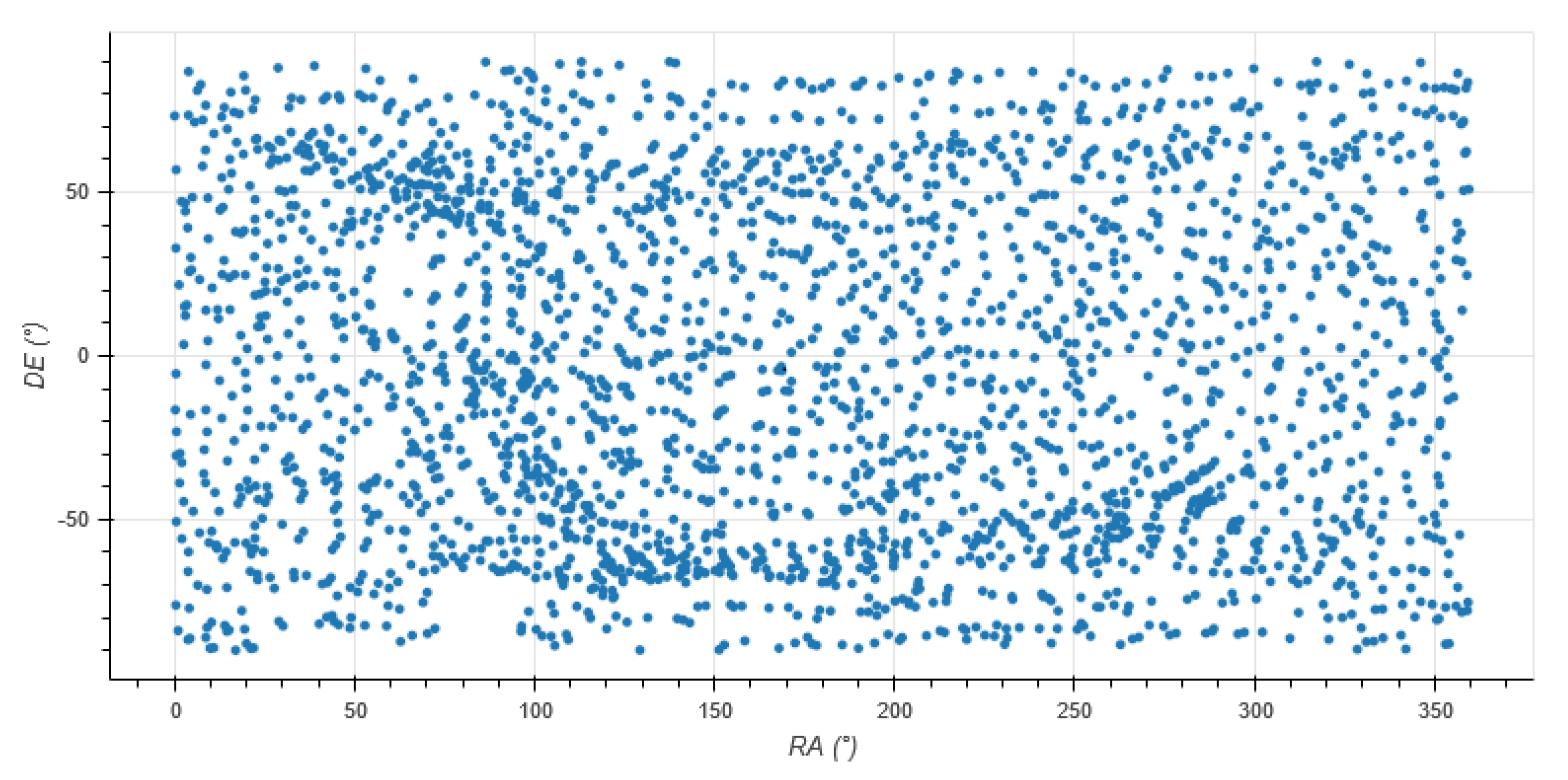
Figure 3.
Distribution of star features in the database.
Figure 3.
Distribution of star features in the database.
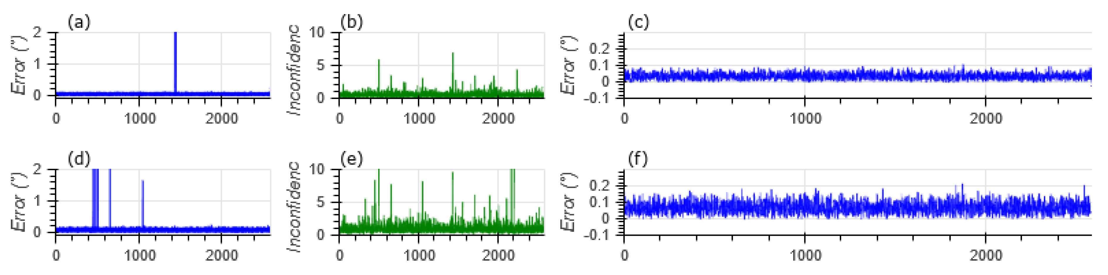
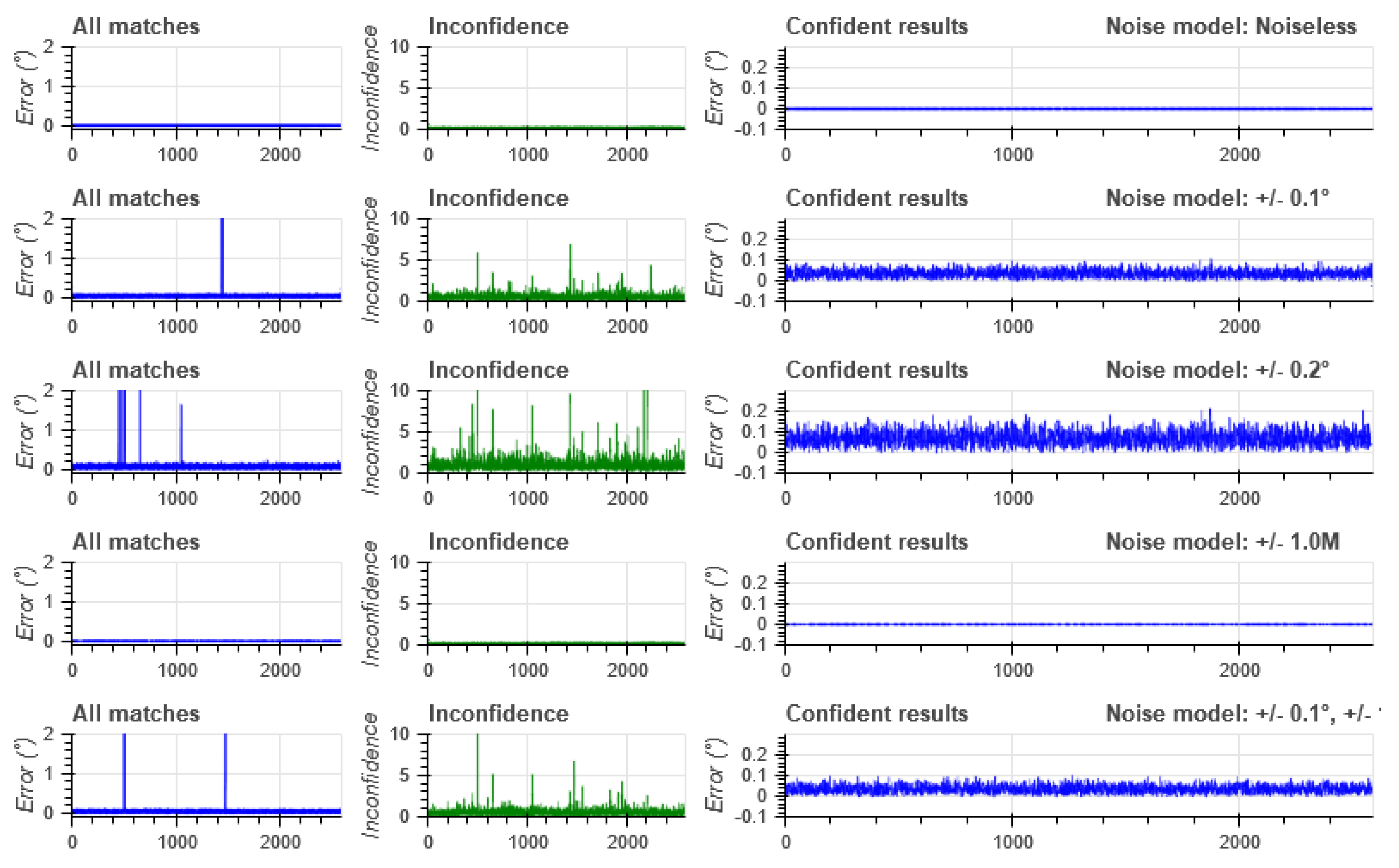
Figure 4.
Star catalog to feature database matching with angular noise: (a) Raw Error with Noise (b) Matching score ( Noise) (c) Error after filtering ( Noise) (d) Raw Error ( Noise) (e) Matching score ( Noise) Noise (f) Error after filtering ( Noise).
Figure 4.
Star catalog to feature database matching with angular noise: (a) Raw Error with Noise (b) Matching score ( Noise) (c) Error after filtering ( Noise) (d) Raw Error ( Noise) (e) Matching score ( Noise) Noise (f) Error after filtering ( Noise).
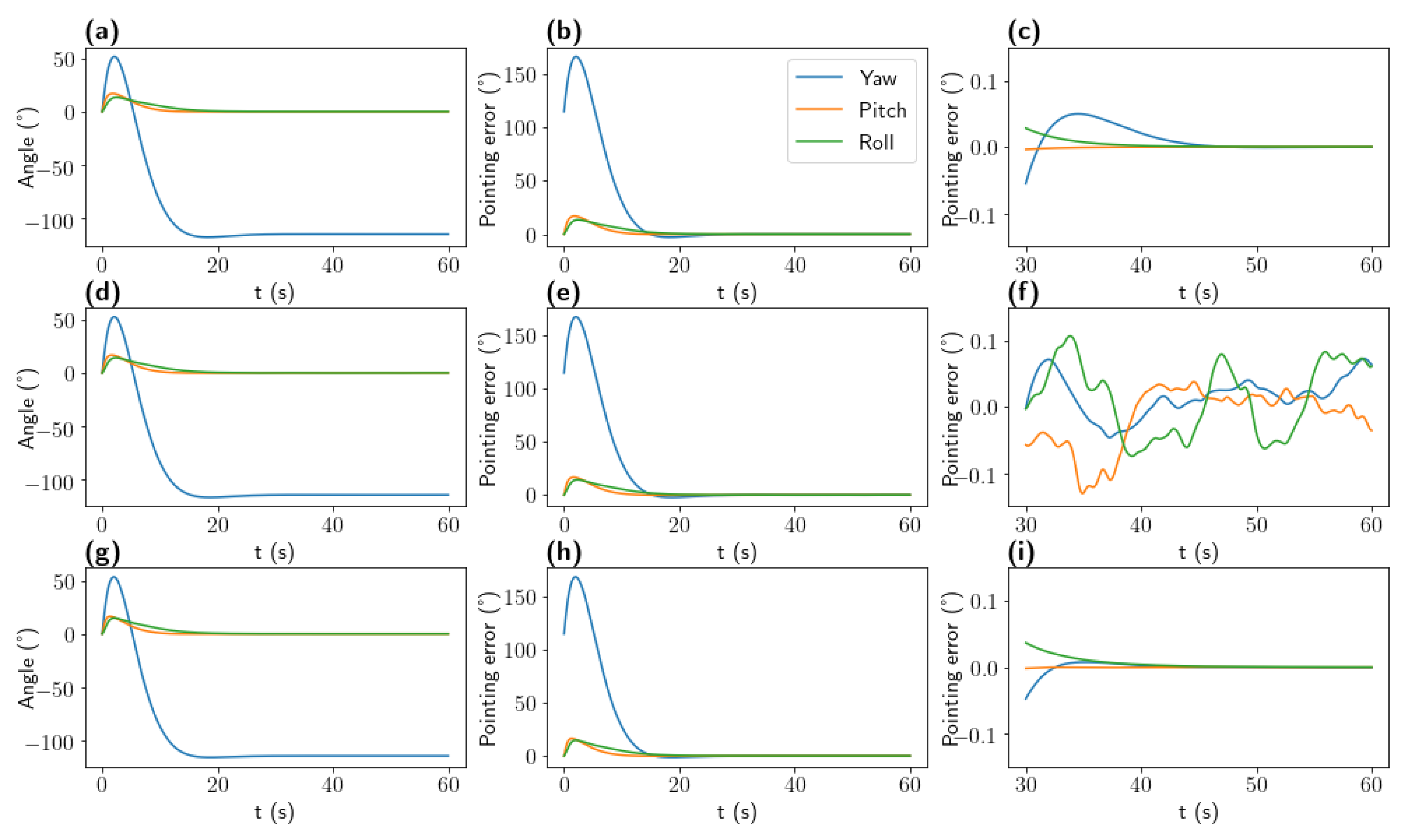
Figure 5.
Pointing accuracy performances of three ADCS; Top (a–c): ADCS with ground truth attitude, Center (d–f): ADCS with 2 Hz Star Tracker and 50 Hz rate gyro Bottom (g–i): ADCS with the proposed Star Tracker, Left (a,d,g) Impulse response, Middle: (b,e,h) Pointing error: (c,f,i) focus on the pointing errors after 30 s.
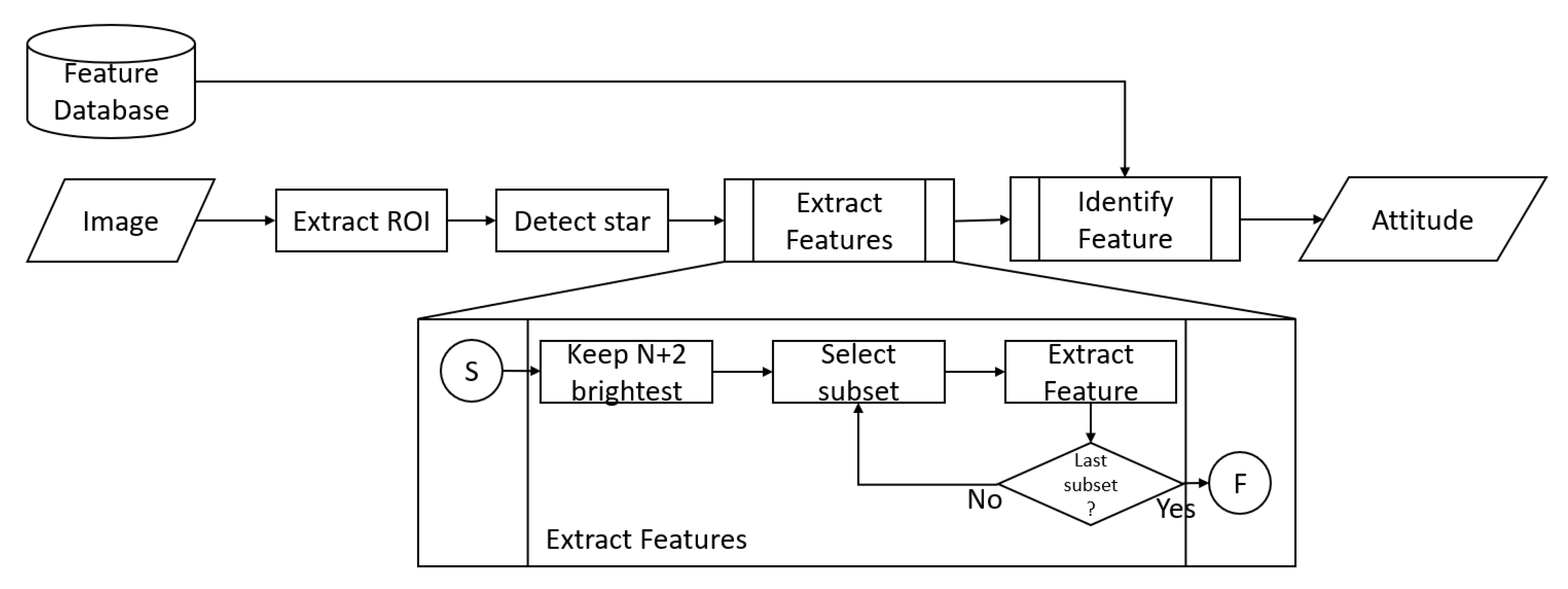
Figure 6.
Flowchart of the proposed Star Tracker image processing pipeline.
Figure 6.
Flowchart of the proposed Star Tracker image processing pipeline.
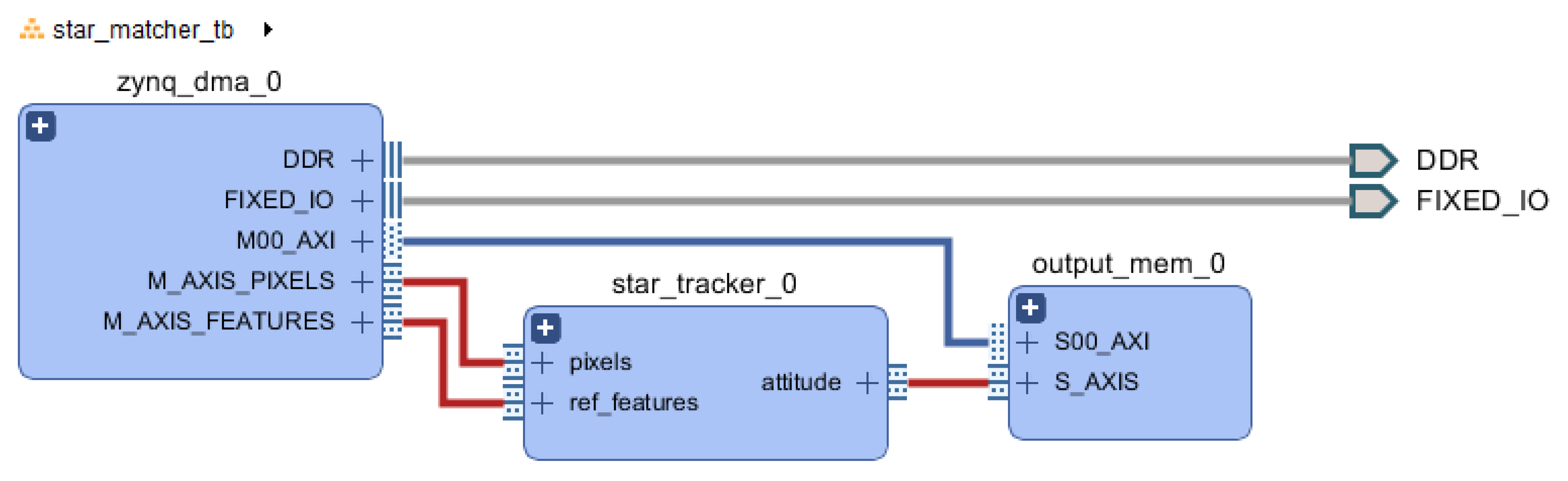
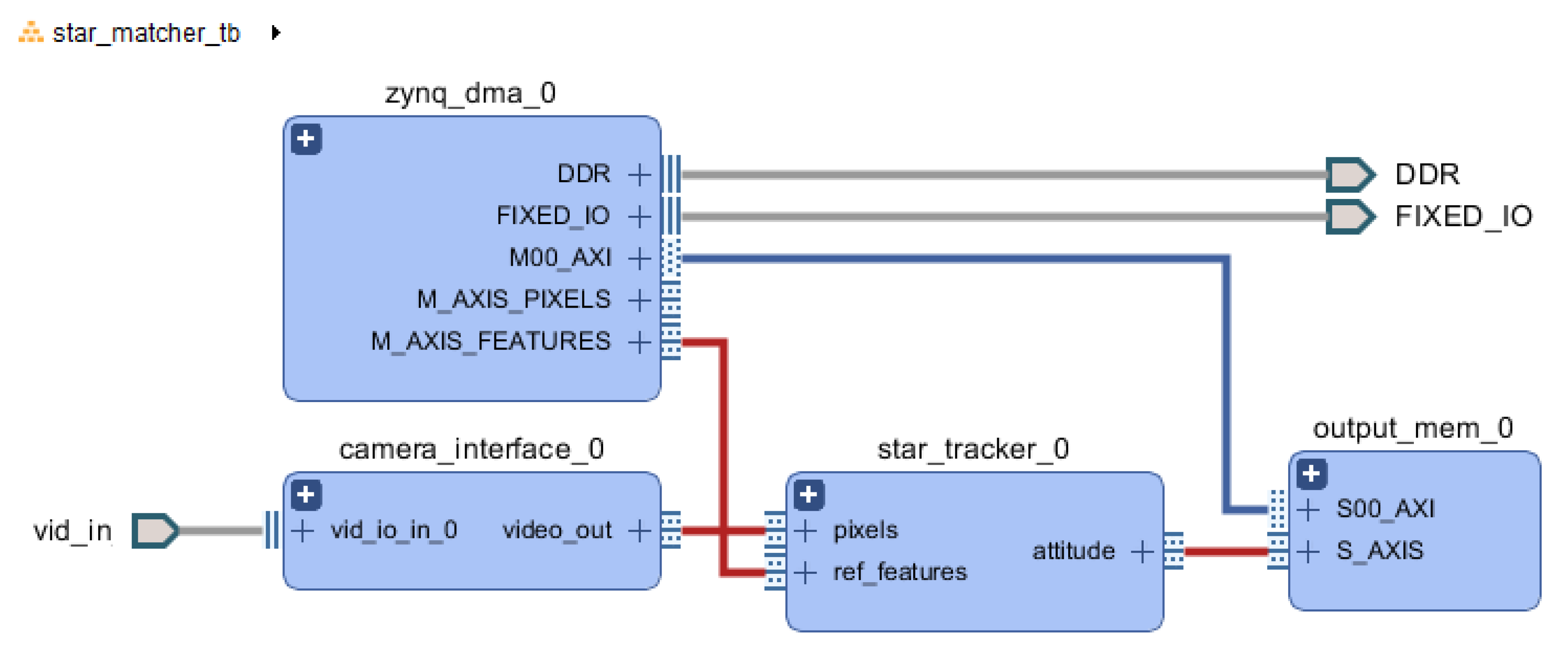
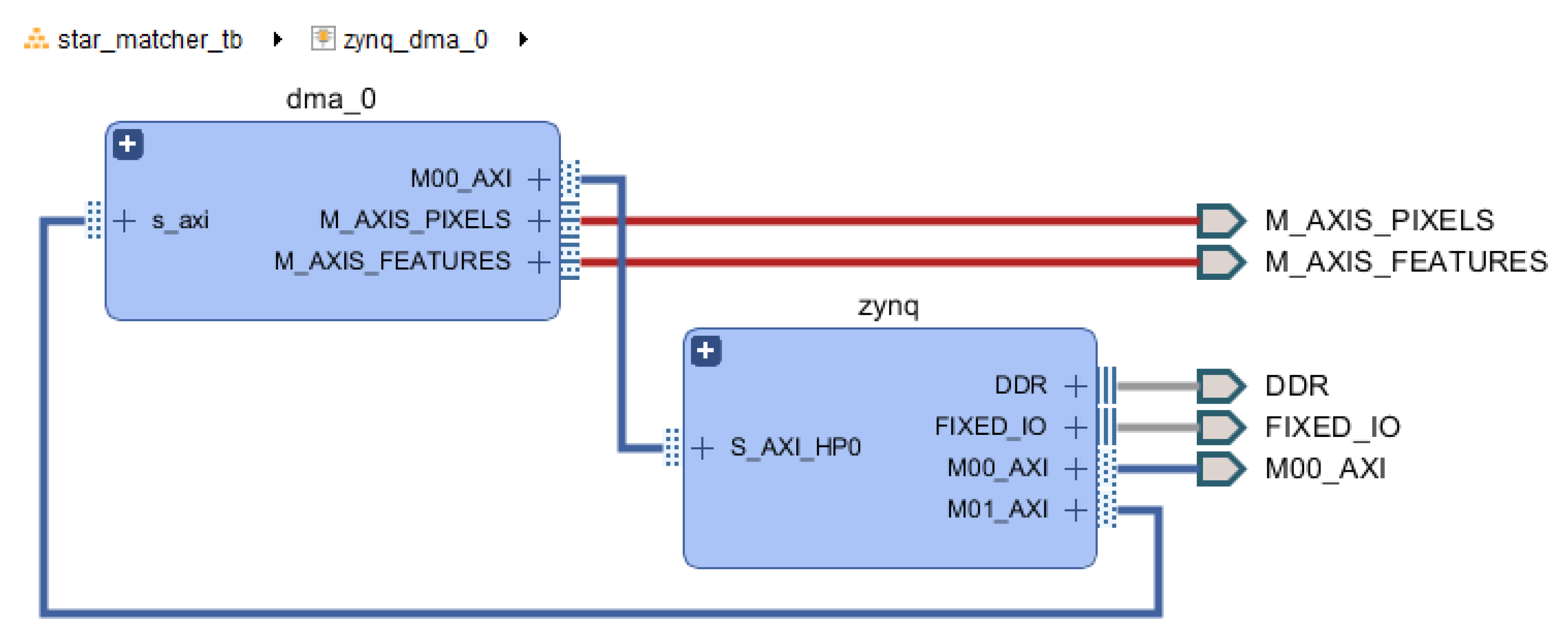
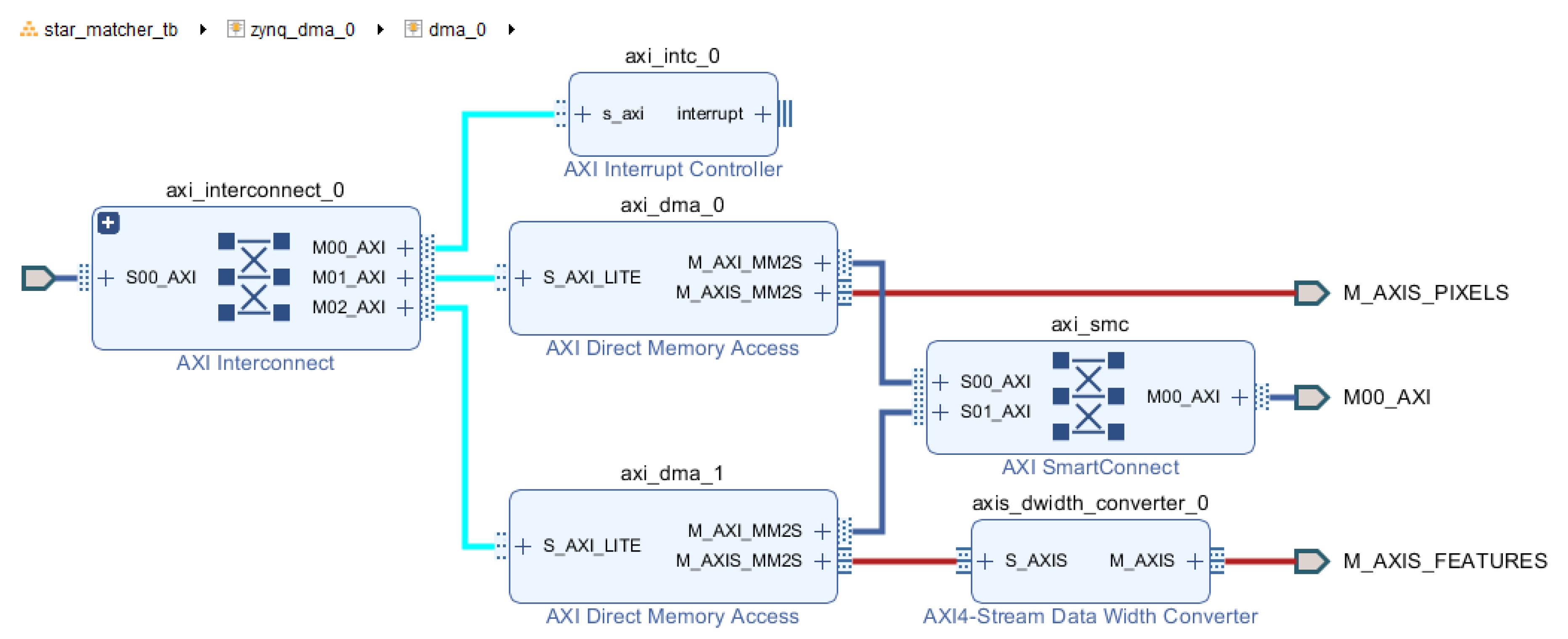
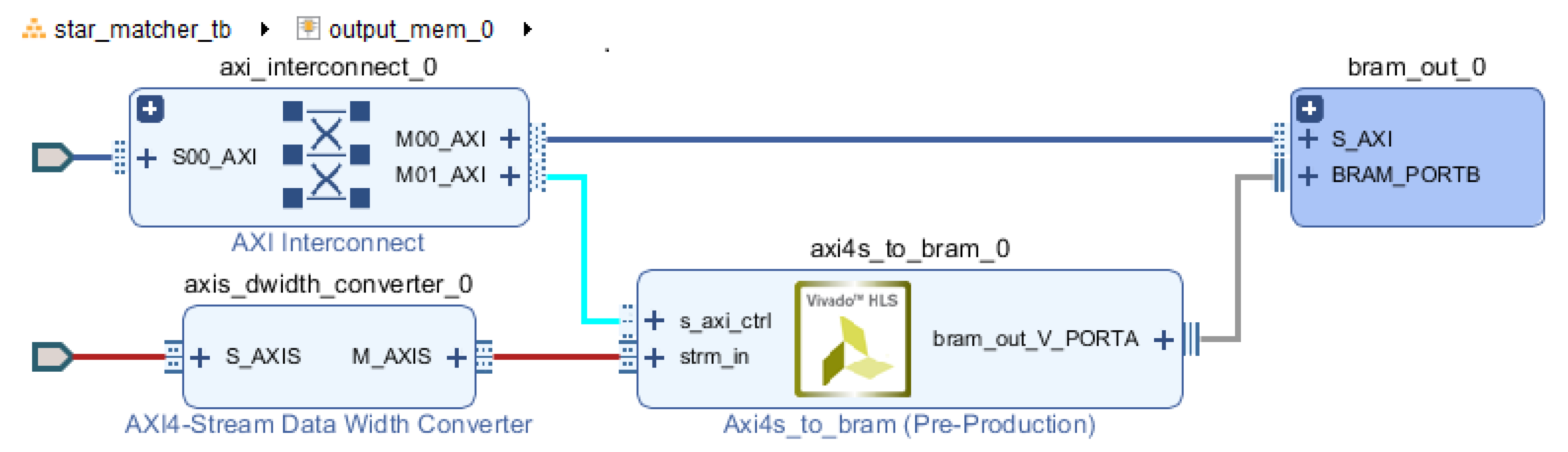
Figure 7.
Top level design of test setup with Zynq.
Figure 7.
Top level design of test setup with Zynq.
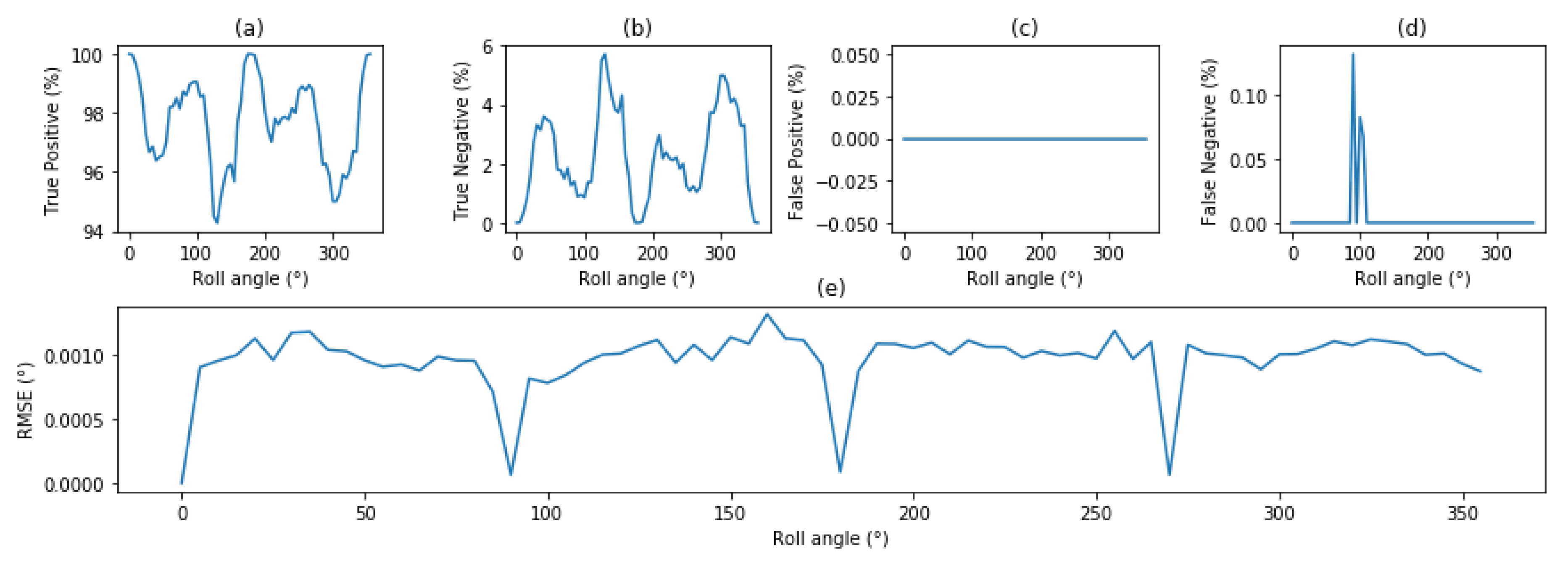
Figure 8.
Evaluation of the performances of the proposed star tracker on 10,000 random images for every 5° of roll angle (a) True-Positive (b) True-negative (c) False-positive (d) False-negatives (e) RMSE of attitude estimation.
Figure 8.
Evaluation of the performances of the proposed star tracker on 10,000 random images for every 5° of roll angle (a) True-Positive (b) True-negative (c) False-positive (d) False-negatives (e) RMSE of attitude estimation.
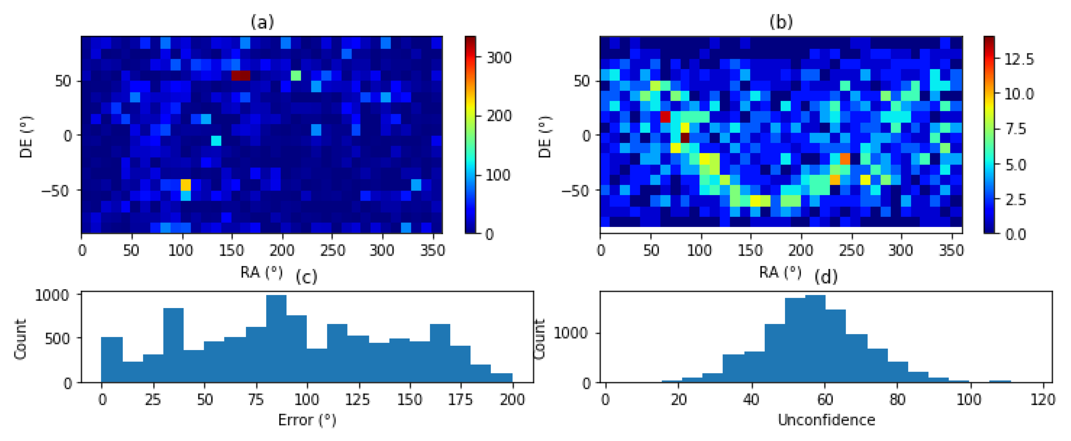
Figure 9.
Analysis of wrongly identified frames for every roll angles (a) 2D Histogram of feature position, (b) Star (mag < 5) 2D histogram, (c) Histogram of error (°), (d) Histogram of confidence.
Figure 9.
Analysis of wrongly identified frames for every roll angles (a) 2D Histogram of feature position, (b) Star (mag < 5) 2D histogram, (c) Histogram of error (°), (d) Histogram of confidence.
Figure 10.
Integration with a Camera on a Zynq system.
Figure 10.
Integration with a Camera on a Zynq system.
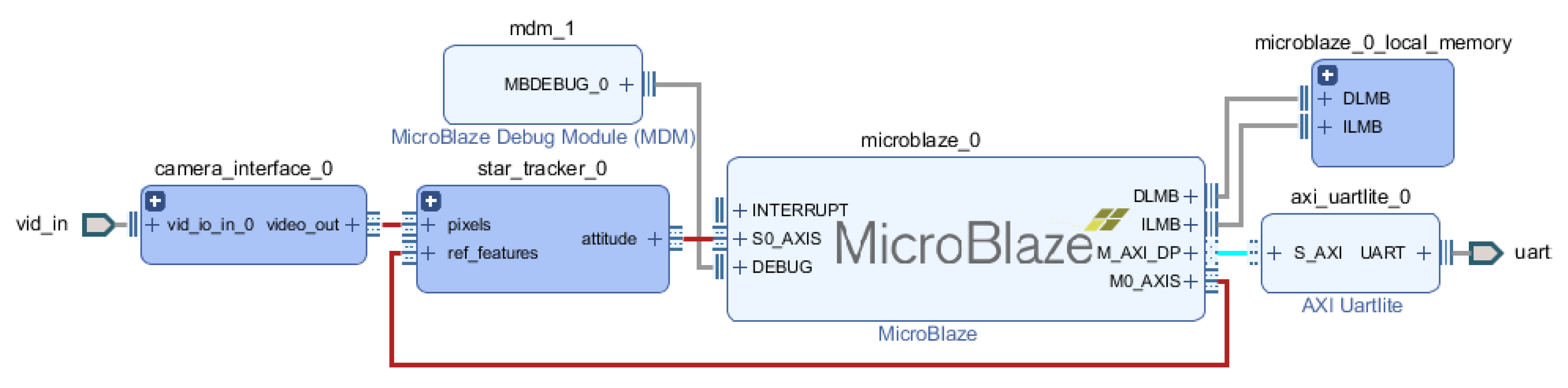
Figure 11.
Integration with a camera without a MicroBlaze soft processor.
Figure 11.
Integration with a camera without a MicroBlaze soft processor.
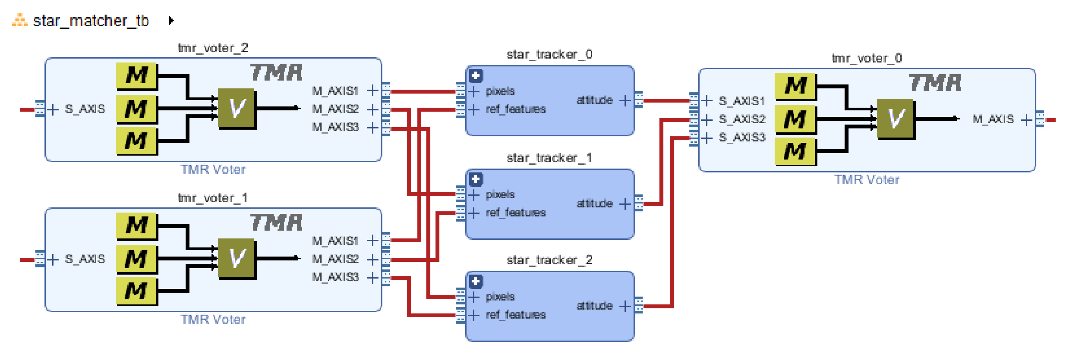
Figure 12.
TMR implementaton on Vivado IP Integrator.
Figure 12.
TMR implementaton on Vivado IP Integrator.
Table 1.
Optical parameters.
Table 1.
Optical parameters.
| T | = | s | Exposure time (50 frames/s) |
| = | 14,000 | Sensor’s Full Well capacity |
| = | | Sensor’s Quantum Efficiency |
| = | | Average Lens Transmission |
| = | or | Lens Aperture and f-number |
| FOV | = | ° or ° | Associated Field of View with given sensor |
| = | | Lens and sensor bandwidth: 300–900 nm |
| = | | Sensitivity, in Electrons per LSB at 14 bits output |
Table 2.
Average center pixel value induced by three stars of apparent magnitude 0, 3 and 5 for 20 ms exposure time with three different PSF.
Table 2.
Average center pixel value induced by three stars of apparent magnitude 0, 3 and 5 for 20 ms exposure time with three different PSF.
| Optics (Focal / f#, FOV) | Star (Hip. id) | V | Center Pixel Value |
|---|
| | | | | | |
| 25/0.9 mm, FOV = 36° | -Lyrae (91262) | +0.03 | 170,007/ | 86,977/ | 27,365/ |
| | -Lyrae (93194) | +3.25 | 8758/ | 4480/ | 1409/ |
| | -Lyrae (93279) | +4.94 | 1846/ | 944/ | 297/ |
| 17/0.9 mm, FOV = 51.6° | -Lyrae (91262) | +0.03 | 78,611/ | 40,218/ | 12,653/ |
| | -Lyrae (93194) | +3.25 | 4049/ | 2071/ | 651/ |
| | -Lyrae (93279) | +4.94 | 853/ | 436/ | 137/ |
Table 3.
Summary of the proposed star identification algorithm’s robustness against noise injection.
Table 3.
Summary of the proposed star identification algorithm’s robustness against noise injection.
| Noise Model | All 2500 Randomly Tested Attitude | Confidence Score < 5 |
|---|
| | RMSE | Mean Error | Confidence Score | % | RMSE | Mean Error |
|---|
| Noiseless | 0.000° | 0.000° | 0.054 | 100.00 | 0.000° | 0.000° |
| ±0.1° | 3.699° | 0.134° | 0.486 | 99.92 | 0.039° | 0.035° |
| ±0.2° | 3.386° | 0.161° | 0.949 | 99.77 | 0.076° | 0.068° |
| ±1.0M | 0.000° | 0.000° | 0.054 | 100.00 | 0.000° | 0.000° |
| ±0.1°, ±1M | 0.040° | 0.034° | 0.482 | 99.92 | 0.038° | 0.034° |
Table 4.
Star Identification Accuracy: summary of 10,000 tests from cropped image.
Table 4.
Star Identification Accuracy: summary of 10,000 tests from cropped image.
| | | | |
|---|
| Wsize | %Confident | RMSE | %Confident | RMSE | %Confident | RMSE |
|---|
| 3 | 84.24% | 0.003878° | 98.84 | 0.000964° | 99.23 | 0.000942° |
| 5 | 81.66% | 0.003821° | 98.81 | 0.000954° | 99.20 | 0.000823° |
| 7 | 83.27% | 0.003861° | 98.78 | 0.000954° | 99.14 | 0.000901° |
Table 5.
Estimation of the impact, magnitude and counter-measure to various noise sources.
Table 5.
Estimation of the impact, magnitude and counter-measure to various noise sources.
| Noise Source | Synergy | Effect on Data | Impact | Effet on the Proposed Star Tracker |
|---|
| Shot Noise | ↗ noise with low V | Noisy stars | + | Noisy detection, centroid, magnitude |
| Sun and Moon | ↗ events with FOV | Occlusion | + | Partial obstruction, lower availability |
| Sun and Moon | ↗ events with FOV | Blooming | + | Reduced availability, increased noise |
| Dark current | ↘ with update rate | Lower readout | – | Noisy detection, centroid, magnitude |
| Thermal noise | ↗ with temperature | Global noise | ∼ | Noisy detection, centroid, magnitude |
| Lens distortion | ↗ with FOV | Wrong position | ∼ | Can be compensated |
| Dead pixels | ↗ with FOV | False Detection | ∼ | Can be excluded |
| Non ideal PSF | ↗ with FOV | Distorted PSF | ∼ | Compensated with large |
| Star motion | ↗ with time | Centroid noise | ∼ | Compensated with an recent database |
| Angular rate | ↗ with exposure | Motion blur | ± | Limits the maximum angular rate |
Table 6.
Analysis of star identification rate and accuracy when subjected to a high angular rate with .
Table 6.
Analysis of star identification rate and accuracy when subjected to a high angular rate with .
| | | | | | |
|---|
Angular
Rate | Spot
Width | Coverage | RMSE | Coverage | RMSE | Coverage | RMSE | Coverage | RMSE |
|---|
| 0°/s | 0 px | 99.4% | 0.00091° | 99.4% | 0.00080° | 99.4% | 0.00080° | 99.4% | 0.00081° |
| 5°/s | 1 px | 99.2% | 0.00114° | 99.2% | 0.00090° | 99.1% | 0.00091° | 99.1% | 0.00091° |
| 10°/s | 2 px | 99.3% | 0.00224° | 99.5% | 0.00117° | 99.4% | 0.00116° | 99.4% | 0.00116° |
| 15°/s | 3 px | 96.7% | 0.00504° | 99.1% | 0.00151° | 99.2% | 0.00151° | 99,2% | 0.00153° |
| 20°/s | 4 px | 87.3% | 0.01008° | 93.7% | 0.00231° | 99.3% | 0.00194° | 99.2% | 0.00197° |
| 30°/s | 6 px | 18.5% | 0.03189° | 18.6% | 0.01163° | 28.3% | 0.00531° | 94.2% | 0.00269° |
Table 7.
Analysis of Baffle length for various optical systems with an Earth Aspect Angle of 30°.
Table 7.
Analysis of Baffle length for various optical systems with an Earth Aspect Angle of 30°.
| Sensor Format | FOV (°) | f/f# (mm) | a (°) | (mm) | (°) | L (mm) |
|---|
| 1″ | 50 | 17/0.95 | 25° | 8.95 | 30 | 161.2 |
| 1″ | 36 | 25/0.95 | 18° | 13.15 | 30 | 104.2 |
| 1″ | 50 | 16/1.40 | 25° | 5.71 | 30 | 102.9 |
| 1″ | 36 | 25/1.40 | 18° | 8.92 | 30 | 70.7 |
Table 8.
Resource usage.
| IP | Slice (%) | LUT as Logic (%) | LUT as Mem (%) | BRAM (%) | DSP (%) |
|---|
| axis_data_fifo | 51 (0.4%) | 27 (0.1%) | 68 (0.4%) | 0.0 (0.0%) | 0.0 (0.0%) |
| extract_roi_3 | 258 (1.9%) | 158 (0.3%) | 640 (3.7%) | 0.0 (0.0%) | 0.0 (0.0%) |
| feature_extractor_st | 1001 (7.5%) | 2497 (4.7%) | 130 (0.7%) | 2.0 (1.4%) | 3.0 (1.4%) |
| feature_matcher_strm | 802 (6.0%) | 1383 (2.6%) | 334 (1.9%) | 3.0 (2.1%) | 0.0 (0.0%) |
| star_detector_3 | 187 (1.4%) | 276 (0.5%) | 12 (0.1%) | 0.0 (0.0%) | 1.0 (0.5%) |
| Total | 2281(17.2%) | 4341 (8.2%) | 1184 (6.8%) | 5.0 (3.6%) | 4.0 (1.8%) |
| Available (XC7Z020) | 13,300 (100%) | 53,200 (100%) | 17,400 (100%) | 140 (100%) | 220 (100%) |
Table 9.
Statistics of database performances for different number of features per frames over 10,000 tests.
Table 9.
Statistics of database performances for different number of features per frames over 10,000 tests.
| k | Total | Unique | Size (kB) | Matching Delay ( s) | Total Time (ms) | Confident | RMSE |
|---|
| 1 | 64,800 | 3221 | 83 | 167 | 15.0 | 9004/10,000 | 0.000299° |
| 2 | 129,600 | 6209 | 161 | 322 | 16.6 | 9586/10,000 | 0.000301° |
| 3 | 194,400 | 9034 | 235 | 469 | 18.1 | 9738/10,000 | 0.000309° |
| 5 | 324,000 | 14,396 | 374 | 748 | 21.0 | 9959/10,000 | 0.000301° |
| 9 | 583,200 | 22,505 | 585 | 1170 | 25.3 | 9990/10,000 | 0.000295° |
| 15 | 972,000 | 32,311 | 840 | 1680 | 30.6 | 9995/10,000 | 0.000305° |
| 21 | 1,360,800 | 39,158 | 1018 | 2076 | 34.1 | 9998/10,000 | 0.000307° |
Table 10.
Comparison between commercially available CubeSat star trackers and the proposed star tracker.
Table 10.
Comparison between commercially available CubeSat star trackers and the proposed star tracker.
| Parameter | MAI-SS Space Sextant | ST400 | Proposed |
|---|
| Interface | I2C | RS422/UART/I2C/SPI | RS485/UART/LVDS |
| FOV | NA | 15° × 18° | 51° or 36° |
| Update rate | 4 Hz | 5 Hz | 25–50 Hz |
| Accuracy | 4 arcsec/27 arcsec | 10 arcsec | 4 arcsec/26 arcsec |
| Compatible OBC | Any | Any | Any or NanoMind Z7000 |
| Power consumption | 1.5 W | 0.7 W | 0.13W FPGA + 0.4 mW Senor |
| Weight | 282 g | 280 g | 250 g |
| Volume | 55 cm × 65 cm × 70 cm | 48 cm × 57 cm × 89 cm | 50 cm × 50 cm × 70 cm |
| Baffle size | 5″ | included | 70–160 mm |
| Manufacturer | MAI | Berlin Space Technologies | NA |
| Retail price | 32,500 $ | NA | NA |


