Determining the Optimal Restricted Driving Zone Using Genetic Algorithm in a Smart City


Abstract
:1. Introduction
- An innovative technique called Optimal Restricted Driving Zone (ORDZ) is introduced that intelligently determines restricted driving zones using a machine learning technique. RDZ reduces traffic load and air pollution, and increase citizens satisfaction who wish to travel by their own vehicle. All the aforementioned objectives are formulated into a single multi-objective function that constitute an evolutionary algorithm called genetic algorithm. While the previous works [8,9] determine restrict zone empirically, ORDZ generates a possible solution iteratively until it reaches the optimal solution (with each episode creating a viable solution). This approach has a significant advantage in dynamic traffic conditions as shown in the following sections.
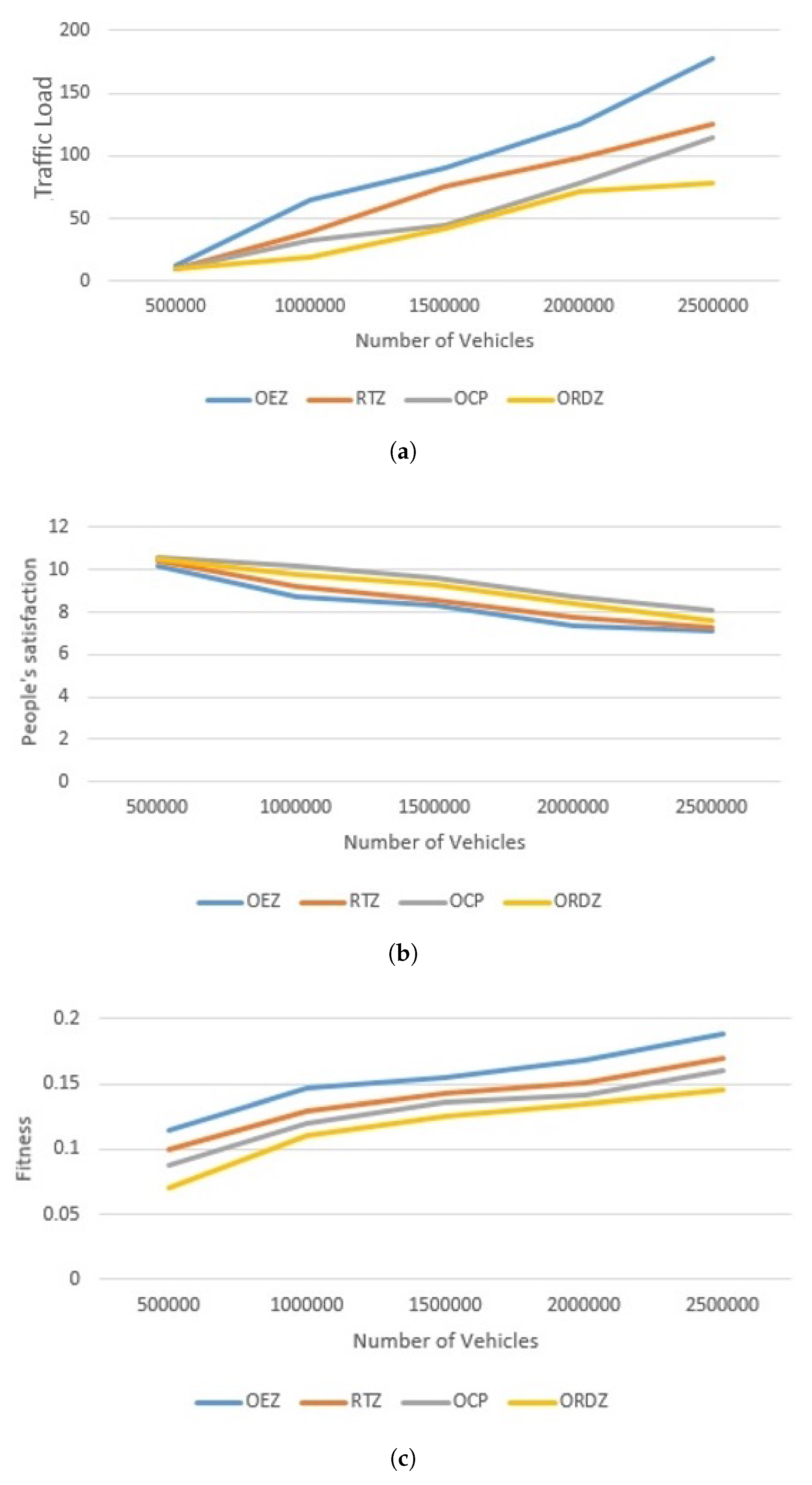
- In our simulation, ORDZ is compared against the other well-known methods including: the Restricted Traffic Zone (RTZ) [8], the Odd-Even Zone (OEZ) [8] and the optimal cordon-based network congestion based on pricing (OCP) [14]. We compare our work against the other well-known empirical approaches. The performance of each method is evaluated with two metrics, traffic load and citizen satisfaction rate. The results show that ORDZ has 23.81% less traffic load than OCP. Also, ORDZ has 22.35% increase in citizen satisfaction than RTZ. We also compare both metrics together as a trade-off and a complete solution. The results show that ORDZ performs 30.6% better than the random modeling, empirical methods, RTZ, OEZ and OCP in terms of traffic load and citizen satisfaction rates.
2. Related Work
2.1. Public Transportation
2.2. Smart Traffic Lights Mmethods
2.3. Modern Technology Method
2.4. Restricted Driving Zone Methods
2.5. Discussion
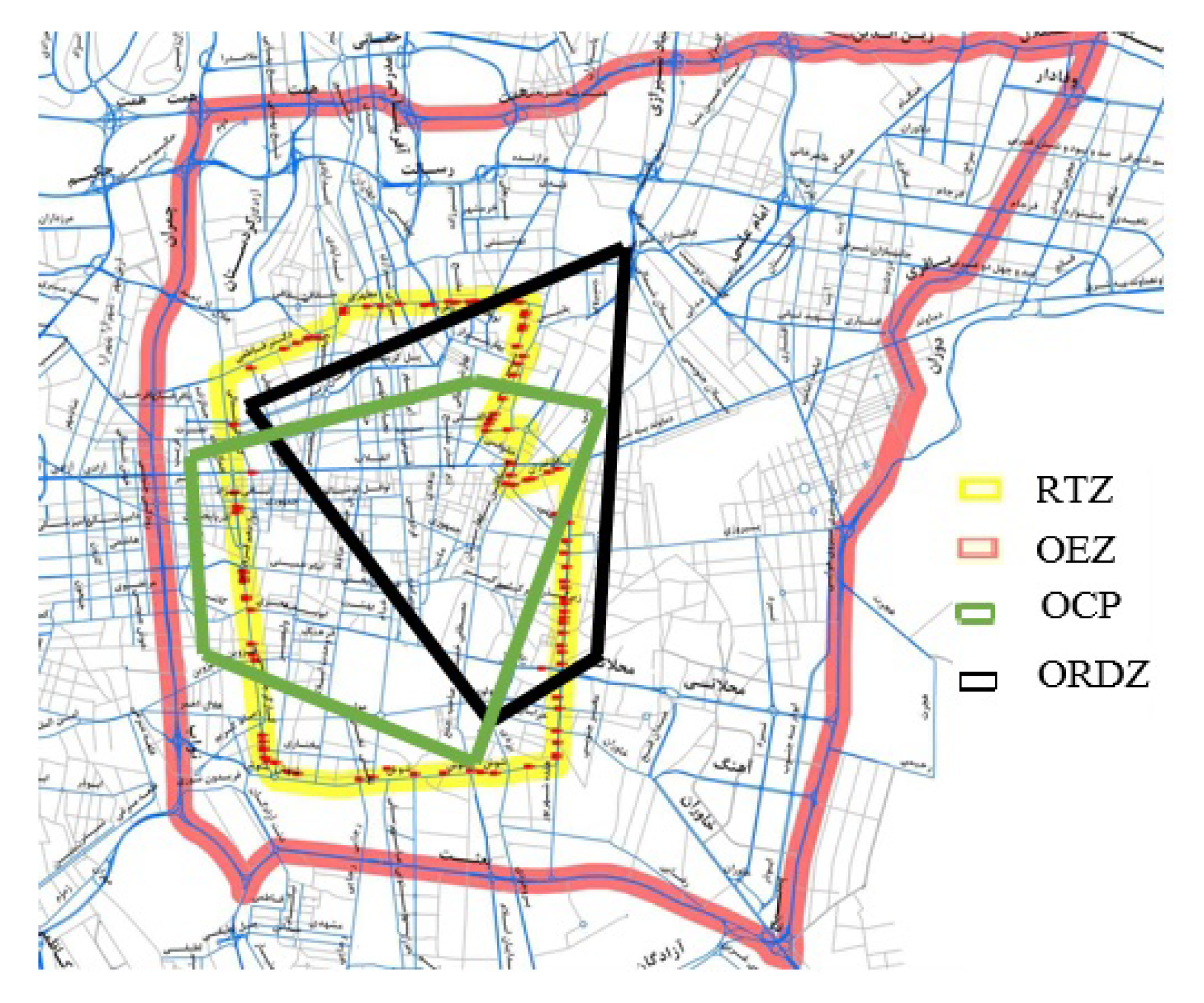
3. System Description
Problem Definition
4. Proposed Method: Optimal Restricted Driving Zone (ORDZ)
4.1. Initial Plan
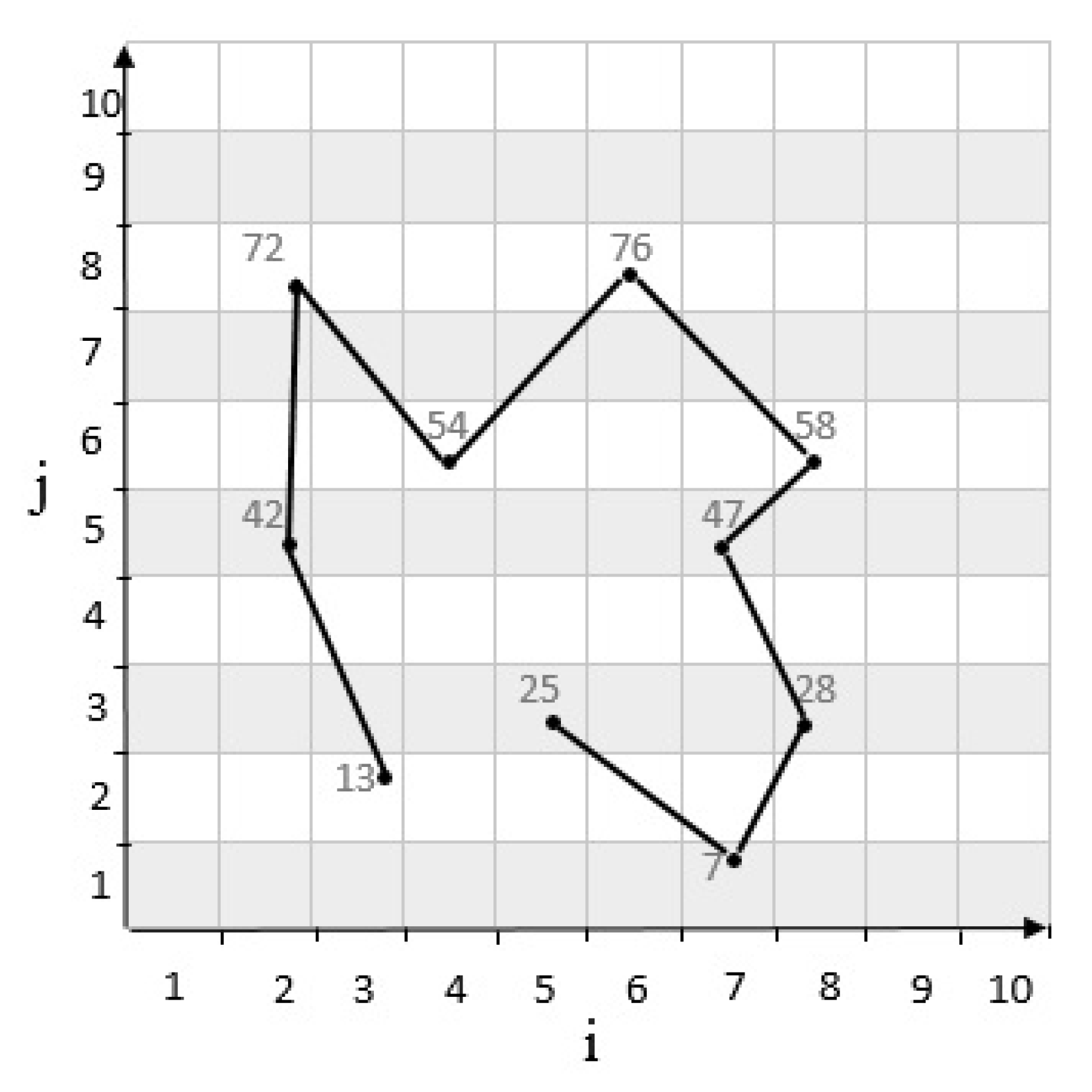
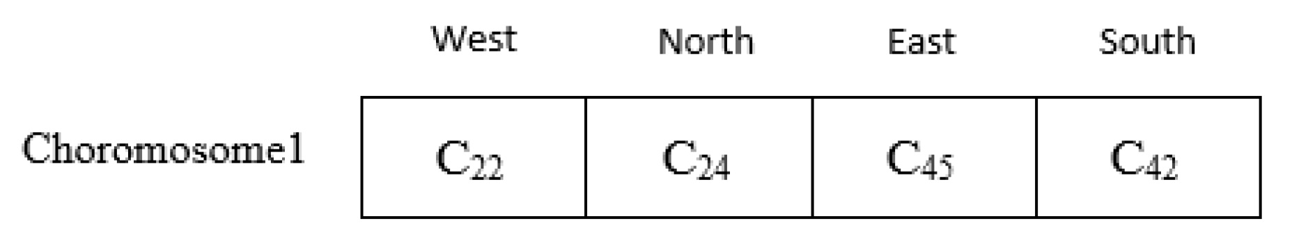
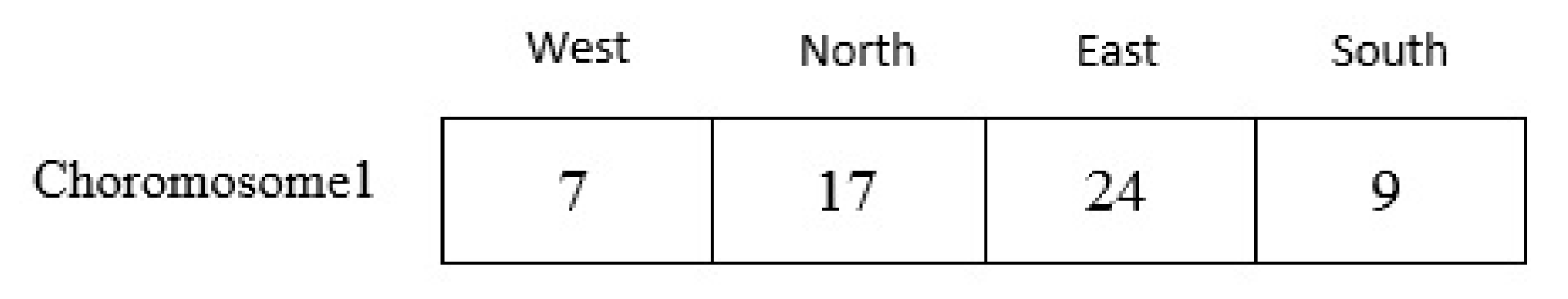
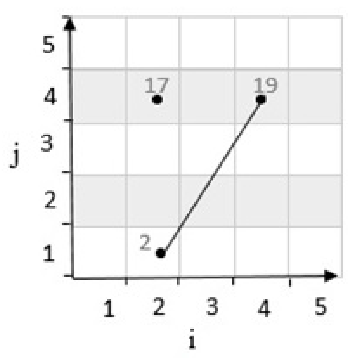
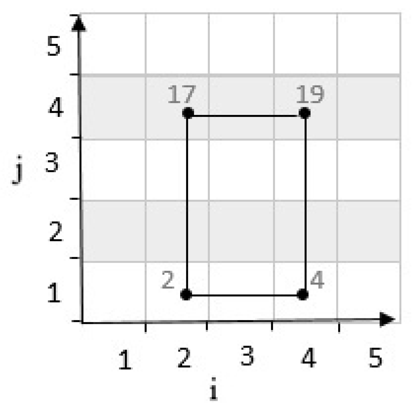
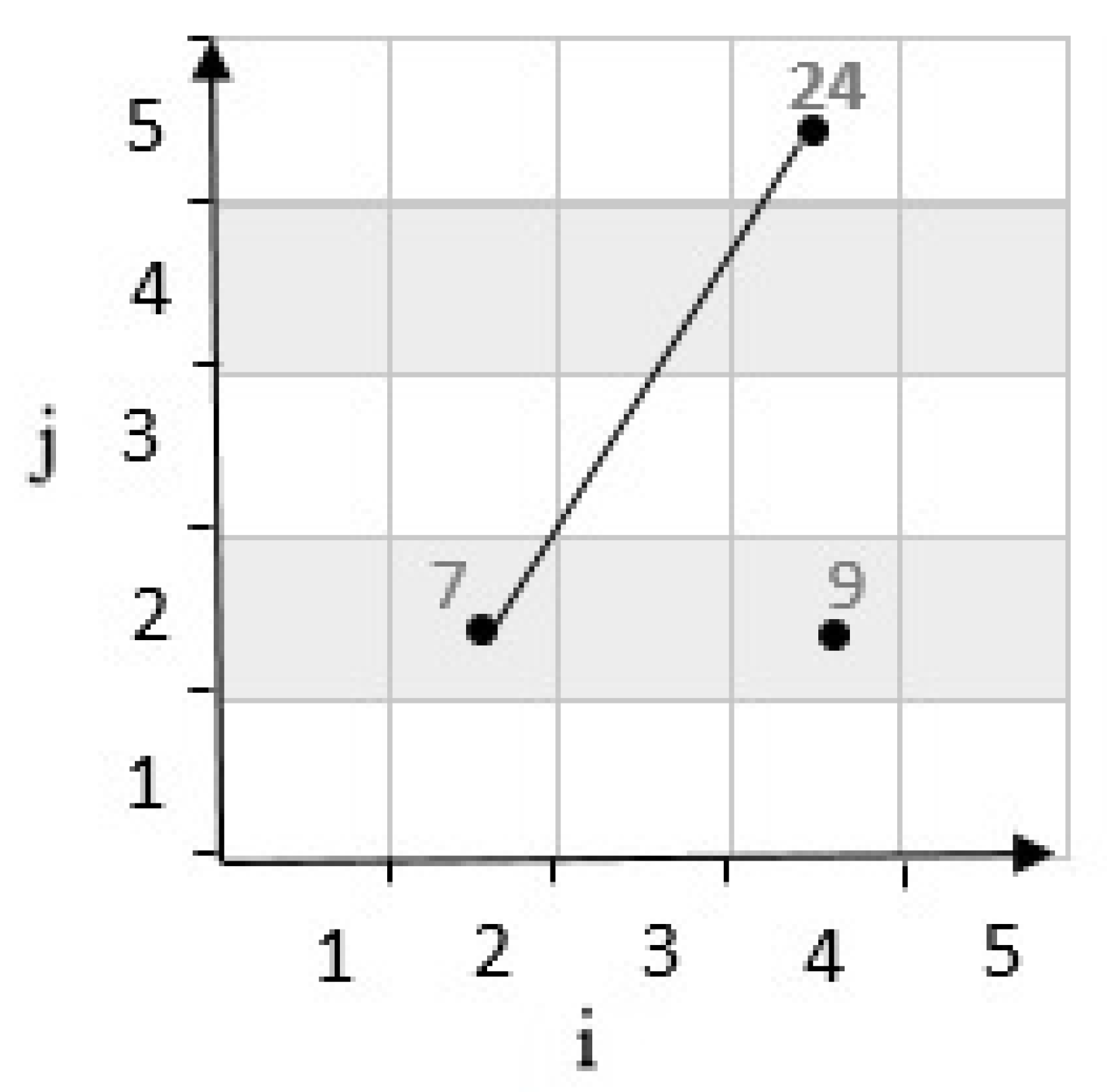
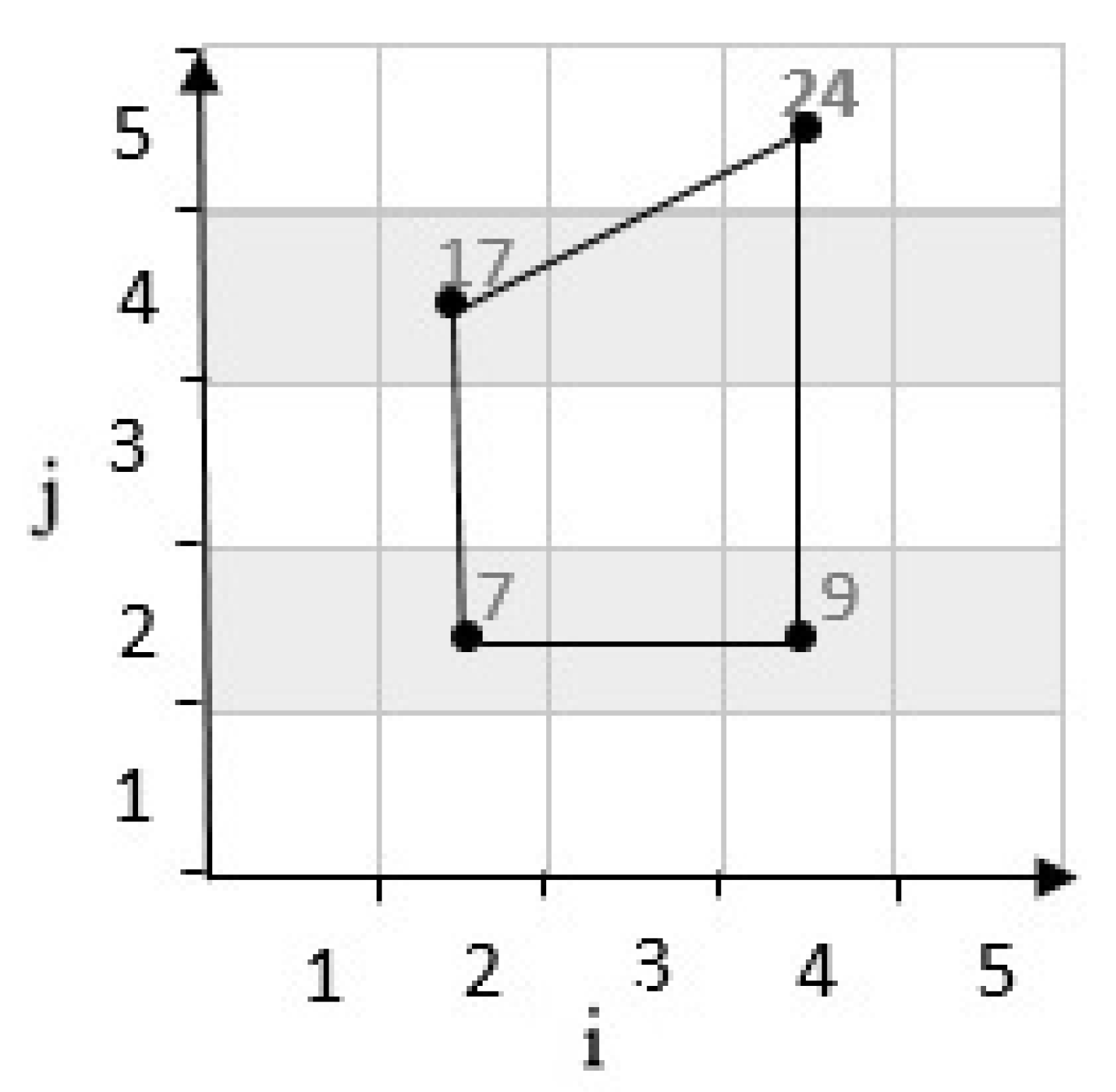
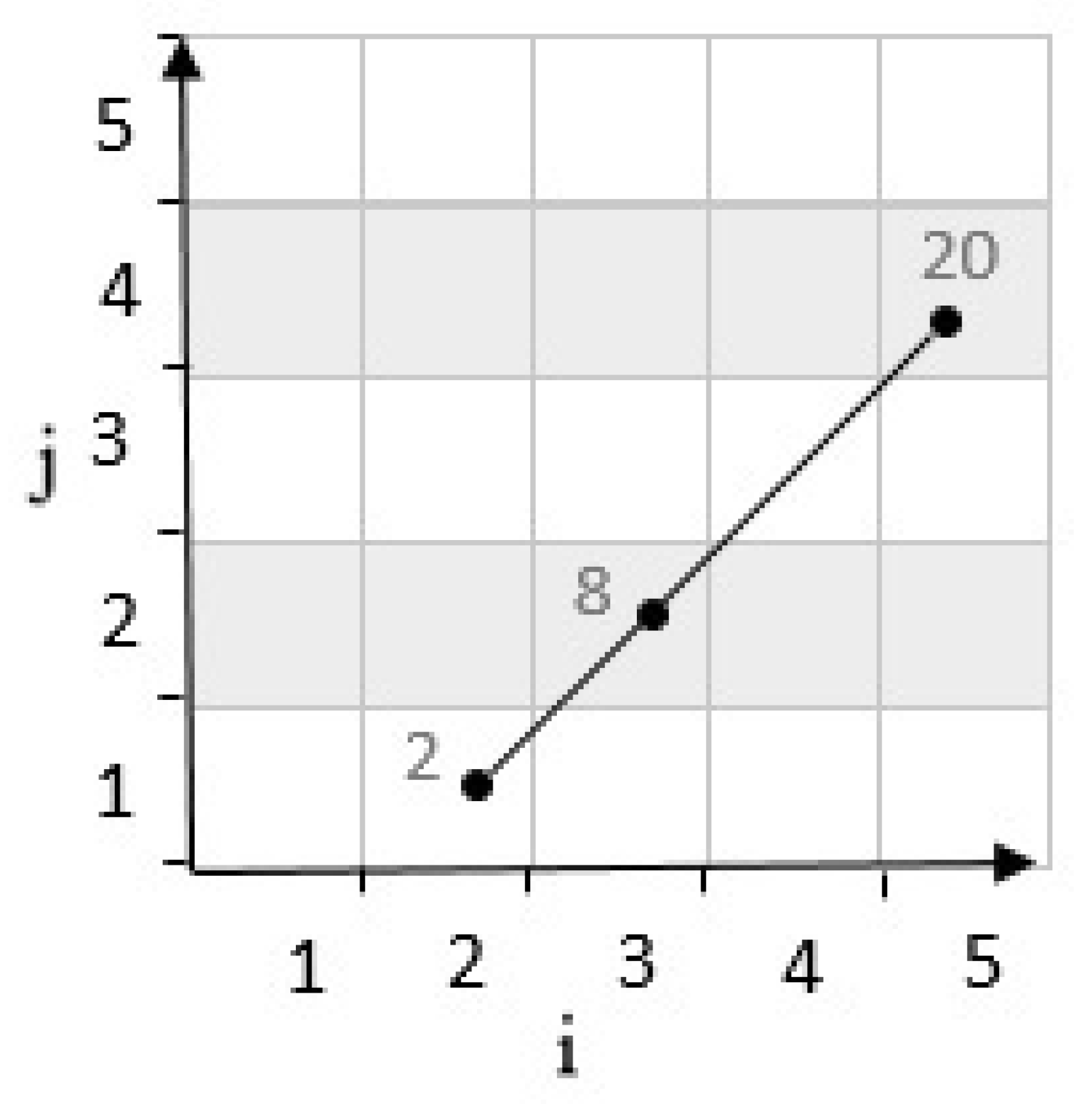
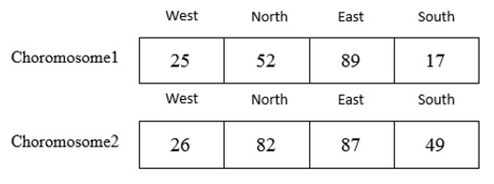
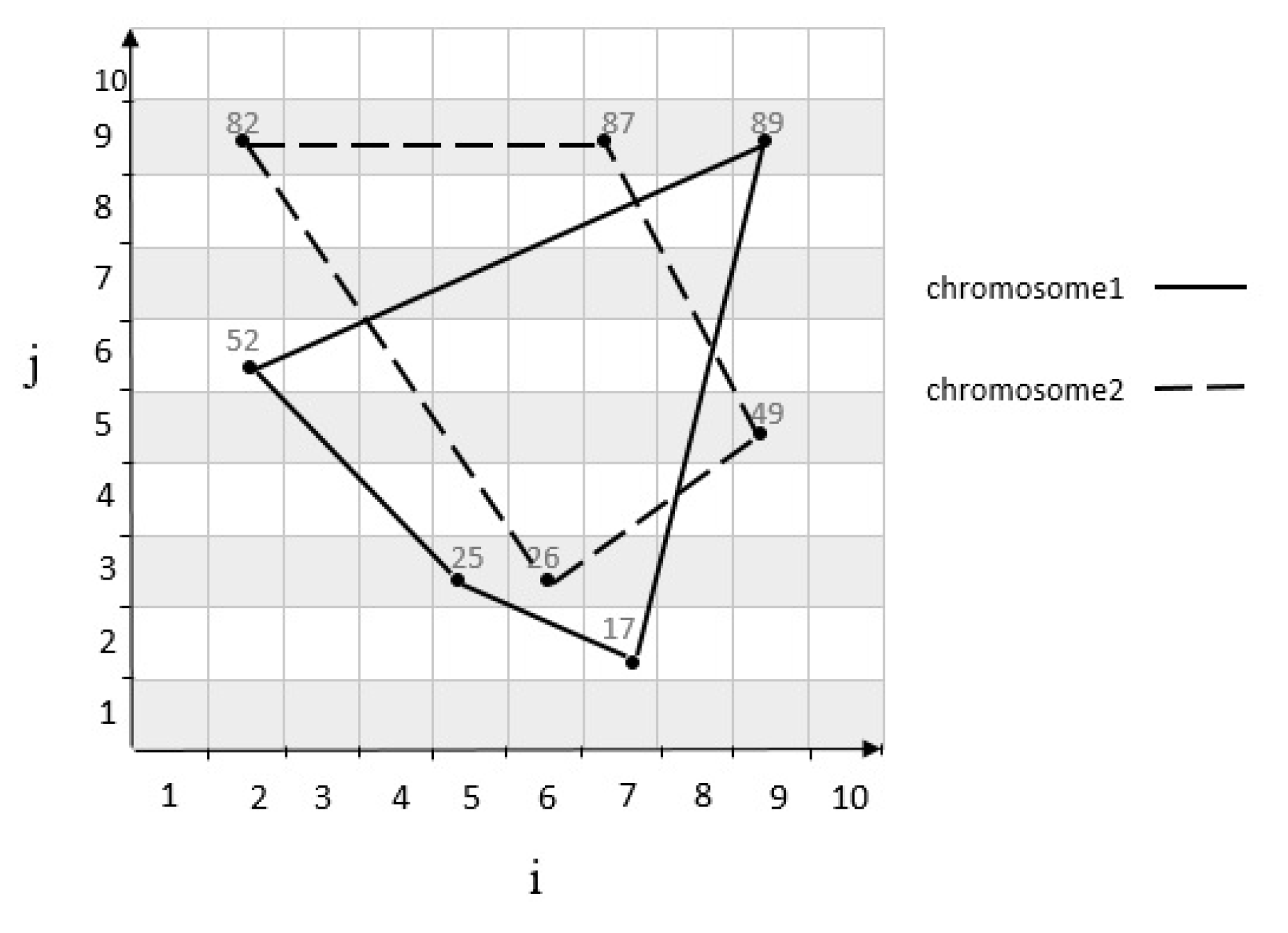
4.2. Chromosome Formulation
4.3. Constraints Satisfaction
4.4. Initial Population
4.5. Parent Selection
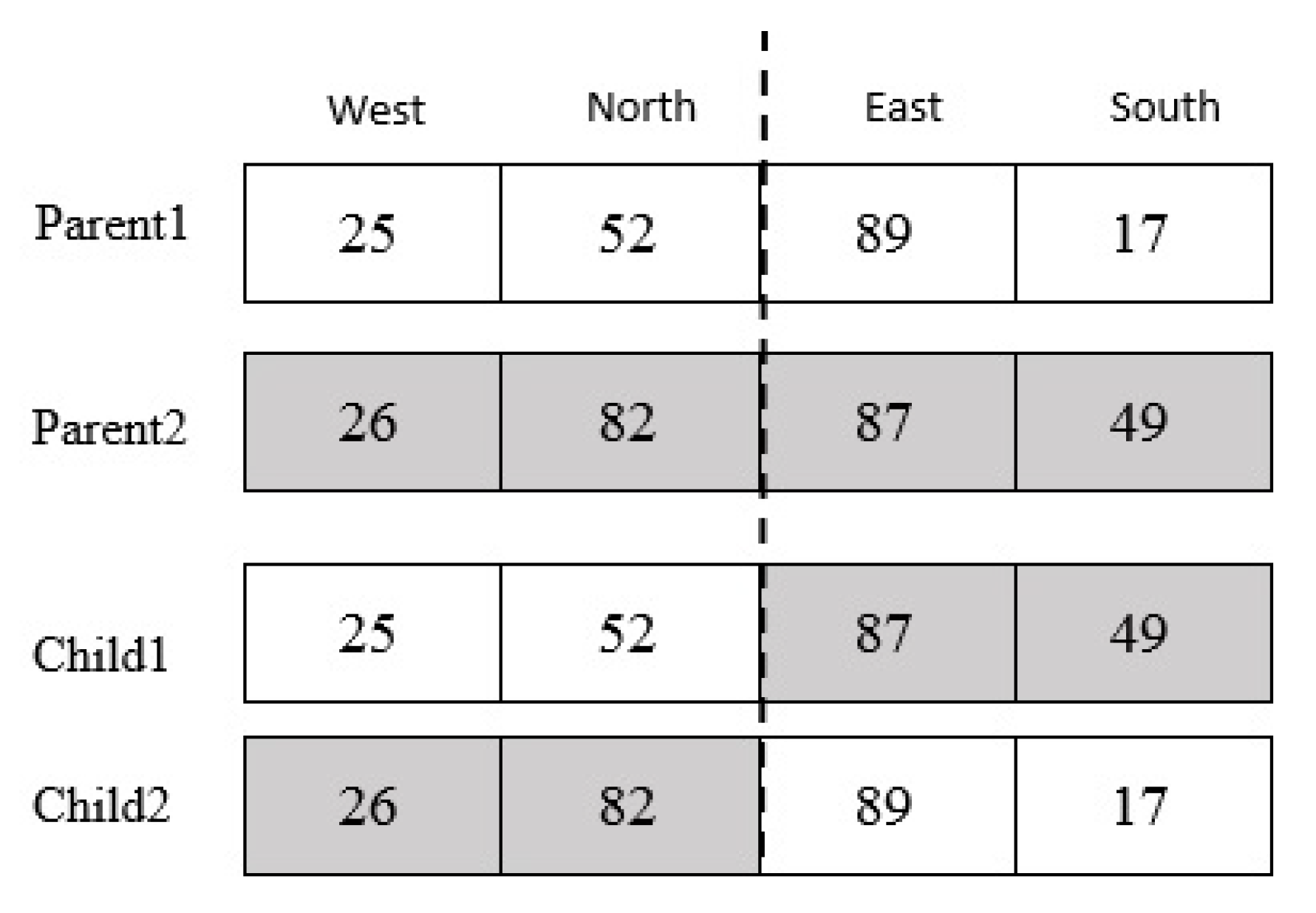
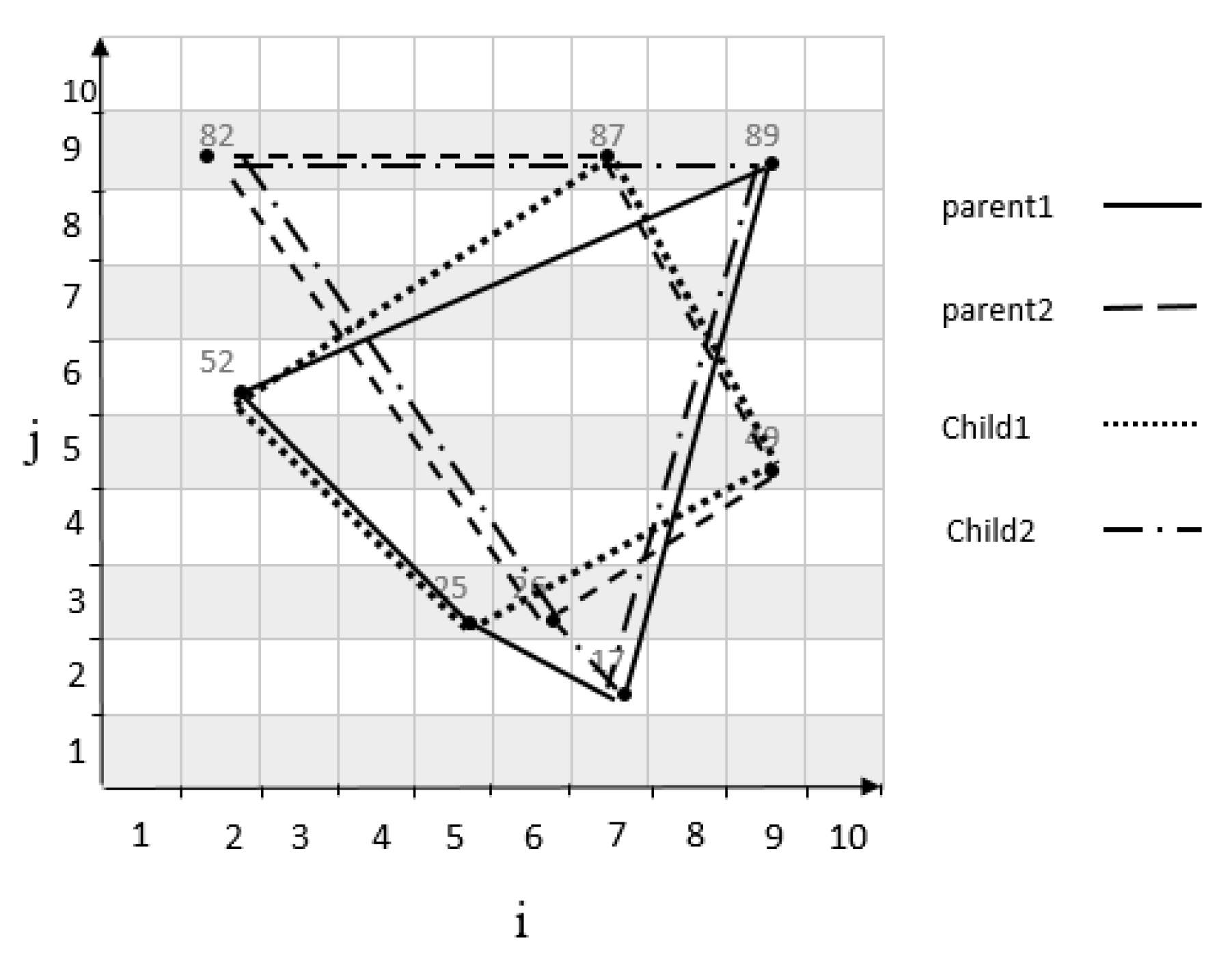
4.6. Crossover
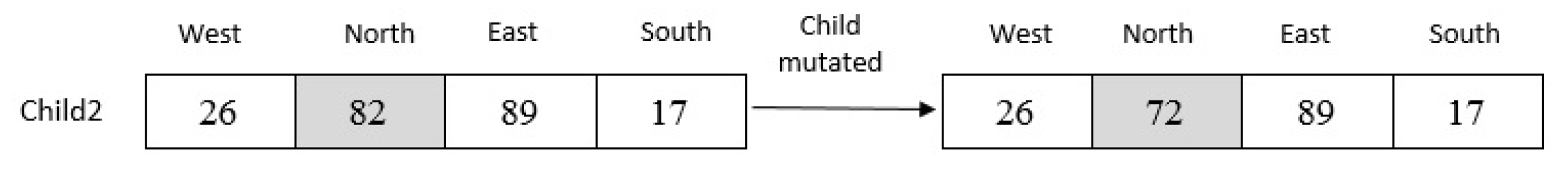
4.7. Mutation
4.8. Fitness Function
4.8.1. Traffic Load
4.8.2. Citizen Satisfaction
4.8.3. Data Normalization
5. Experiments
5.1. First Scenario
5.2. Second Scenario
6. Conclusions
Author Contributions
Funding
Conflicts of Interest
References
- Barth, M.; Boriboonsomsin, K. Real-World CO2 Impacts of Traffic Congestion. In Proceedings of the 87th Annual Meeting of the Transportation Research Board, Washington, DC, USA, 13–17 January 2008; Volume 2058, pp. 163–171. [Google Scholar]
- Chuang, K.J.; Chan, C.C.; Su, T.C.; Lee, C.T.; Tang, C.S. The effect of urban air pollution on inflammation, oxidative stress, coagulation, and autonomic dysfunction in young adults. Am. J. Respir. Crit. Care Med. 2007, 176, 370–376. [Google Scholar] [CrossRef] [PubMed]
- Chen, L.; Xu, J.; Zhang, Q.; Wang, Q.; Xue, Y.; Ren, C. Evaluating impact of air pollution on different diseases in Shenzhen, China. IBM J. Res. Dev. 2017, 61, 1–2. [Google Scholar] [CrossRef]
- John, R.M.; Francis, F.; Neelankavil, J.; Antony, A.; Devassy, A.; Jinesh, K.J. Smart public transport system. In Proceedings of the 2014 International Conference on Embedded Systems (ICES), Coimbatore, India, 3–5 July 2014; pp. 166–170. [Google Scholar]
- Alam, J.; Manjo, D.M. Advance traffic light system based on congestion estimation using fuzzy logic. Int. J. Emerg. Technol. Adv. Eng. 2014, 4, 870–877. [Google Scholar]
- Arora, M.; Banga, V.K. Intelligent traffic light control system using morphological edge detection and fuzzy logic. In Proceedings of the International Conference on Intelligent Computational Systems (ICICS’2012), Dubai, UAE, 7–8 January 2012; pp. 7–8. [Google Scholar]
- Soret, A.; Guevara, M.; Baldasano, J. The potential impacts of electric vehicles on air quality in the urban areas of Barcelona and Madrid (Spain). Atmos. Environ. 2014, 99, 51–63. [Google Scholar] [CrossRef]
- Salarvandian, F.; Dijst, M.; Helbich, M. Impact of traffic zones on mobility. J. Transp. Land Use 2017, 10, 965–982. [Google Scholar] [CrossRef] [Green Version]
- Eguiguren, P. The 2008 Beijing Olympic Games: Spillover Effects on Air Quality and Health. Chicago Policy Review (Online). Available online: https://www.chicagopolicyreview.org (accessed on 12 February 2016).
- Ma, H.; He, G. Effects of the post-olympics driving restrictions on air quality in Beijing. Sustainability 2016, 8, 902. [Google Scholar] [CrossRef] [Green Version]
- Chhatpar, P.; Doolani, N.; Shahani, S.; Priya, R.L. Machine Learning Solutions to Vehicular Traffic Congestion. In Proceedings of the 2018 International Conference on Smart City and Emerging Technology (ICSCET), Mumbai, India, 5 January 2018; pp. 1–4. [Google Scholar]
- Ma, J.; Huang, X.; Jiang, Y. Applicable research of urban road traffic congestion based on rough set theory and Genetic Algorithm. In Proceedings of the World Automation Congress 2012, Puerto Vallarta, Mexico, 24–28 June 2012; pp. 1–4. [Google Scholar]
- Lambora, A.; Gupta, K.; Chopra, K. Genetic Algorithm—A Literature Review. In Proceedings of the 2019 International Conference on Machine Learning, Big Data, Cloud and Parallel Computing (COMITCon), Faridabad, India, 14–16 February 2019; pp. 380–384. [Google Scholar]
- Zhang, X.; Yang, H. The optimal cordon-based network congestion pricing problem. Transp. Res. B Meth. 2004, 38, 517–537. [Google Scholar] [CrossRef]
- Anwar, A.M. Paradox between public transport and private car as a modal choice in policy formulation. J. Bangladesh Inst. Plan. 2009, 2, 71–77. [Google Scholar] [CrossRef] [Green Version]
- Le, T.P.L.; Trinh, T.A. Encouraging public transport use to reduce traffic congestion and air pollutant: A case study of Ho Chi Minh City. Procedia Eng. 2016, 142, 236–243. [Google Scholar] [CrossRef] [Green Version]
- Geng, Y.; Cassandras, C.G. Multi-intersection traffic light control with blocking. Discret. Event Dyn. Syst. 2015, 25, 7–30. [Google Scholar] [CrossRef]
- Mehan, S.; Sharma, V. Development of traffic light control system based on fuzzy logic. In Proceedings of the International Conference on Advances in Computing and Artificial Intelligence, Punjab, India, 21–22 July 2011; pp. 162–165. [Google Scholar]
- Ullah, M.H.; Gunawan, T.S.; Sharif, M.R.; Muhida, R. Design of environmental friendly hybrid electric vehicle. In Proceedings of the 2012 International Conference on Computer and Communication Engineering (ICCCE), Kuala Lumpur, Malaysia, 3–5 July 2012; pp. 544–548. [Google Scholar]
- Zhang, Q.; Chang, S. An Improved Crossover Operator of Genetic Algorithm. In Proceedings of the 2009 Second International Symposium on Computational Intelligence and Design, Changsha, China, 12–14 December 2009; Volume 2, pp. 82–86. [Google Scholar]
- Lim, S.M.; Sultan, A.B.M.; Sulaiman, M.N.; Mustapha, A.; Leong, K.Y. Crossover and mutation operators of genetic algorithms. Int. J. Mach. Learn. Cybern. 2017, 7, 9–12. [Google Scholar] [CrossRef] [Green Version]
- Singh, B.K.; Verma, K.; Thoke, A. Investigations on impact of feature normalization techniques on classifier’s performance in breast tumor classification. Int. J. Comput. Appl. 2015, 116, 11–15. [Google Scholar]
- Keränen, A.; Ott, J.; Kärkkäinen, T. The ONE simulator for DTN protocol evaluation. In Proceedings of the 2nd International Conference on Simulation Tools and Techniques, Rome, Italy, 2–6 March 2009; pp. 1–10. [Google Scholar]
- Behruz, H.; Safaie, A.; Chavoshy, A.P. Tehran traffic congestion charging management: A success story. WIT Trans. Built Environ. 2012, 128, 445–456. [Google Scholar]
- Lieu, H.; Gartner, N.; Messer, C.; Rathi, A. Traffic flow theory. Public Roads 1999, 62, 45–47. [Google Scholar]
- Iranmanesh, S.; Chin, K.W. A novel mobility-based routing protocol for semi-predictable disruption tolerant networks. Int. J. Wirel. Inf. Netw. 2015, 22, 138–146. [Google Scholar] [CrossRef] [Green Version]


| Methods | Advantages | Disadvantages |
|---|---|---|
| Classic methods | • Reduce traffic volume • Reduce air pollution • Low cost | • Low quality • Low satisfaction • High travel time |
| Smart traffic lights methods | • Reduce delay time • Reduce traffic volume • Reduce air pollution | • High maintenance cost |
| Limited traffic zone methods | • Reduce traffic volume • Reduce air pollution • Low travel time | • Low satisfaction • Pay toll |
| Modern Technology Methods | • Reduce air pollution • Reduce Traffic volume • Environment friendly | • High maintenance cost |
| Notation | Description |
|---|---|
| Total number of grid cells | |
| Grid cells | |
| Vehicles | |
| i -th vehicle movement pattern | |
| Discrete time | |
| Couple-time vehicle movement pattern | |
| R | Determinant of matrix |
| Probability of selection each chromosome | |
| Superiority of each chromosome | |
| Initial population | |
| Traffic load | |
| citizen satisfaction rate | |
| Fitness function | |
| Total number of vehicles entering a cell | |
| Average traffic | |
| Z | Data normalization |
| Standard deviation |
© 2020 by the authors. Licensee MDPI, Basel, Switzerland. This article is an open access article distributed under the terms and conditions of the Creative Commons Attribution (CC BY) license (http://creativecommons.org/licenses/by/4.0/).
Share and Cite
Jan, T.; Azami, P.; Iranmanesh, S.; Ameri Sianaki, O.; Hajiebrahimi, S. Determining the Optimal Restricted Driving Zone Using Genetic Algorithm in a Smart City. Sensors 2020, 20, 2276. https://doi.org/10.3390/s20082276
Jan T, Azami P, Iranmanesh S, Ameri Sianaki O, Hajiebrahimi S. Determining the Optimal Restricted Driving Zone Using Genetic Algorithm in a Smart City. Sensors. 2020; 20(8):2276. https://doi.org/10.3390/s20082276
Chicago/Turabian StyleJan, Tony, Pegah Azami, Saeid Iranmanesh, Omid Ameri Sianaki, and Shiva Hajiebrahimi. 2020. "Determining the Optimal Restricted Driving Zone Using Genetic Algorithm in a Smart City" Sensors 20, no. 8: 2276. https://doi.org/10.3390/s20082276