A New Model for Predicting Rate of Penetration Using an Artificial Neural Network


Abstract
:1. Introduction
Artificial Neural Network and its Application in Drilling Operation
2. Data Description
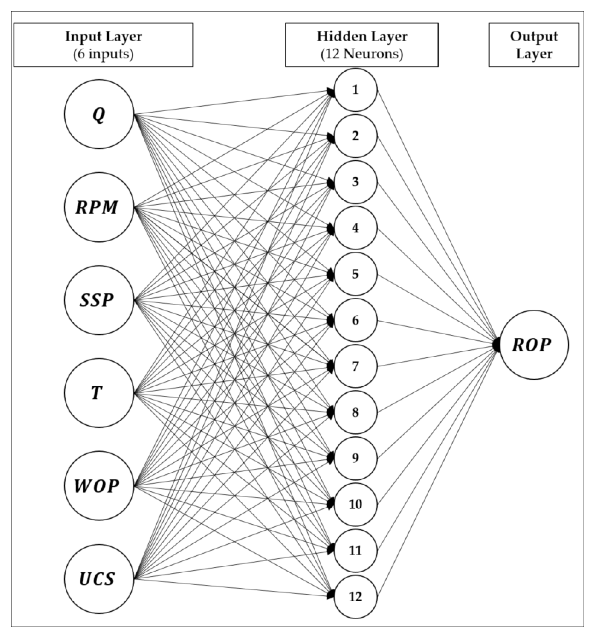
3. ANN Model
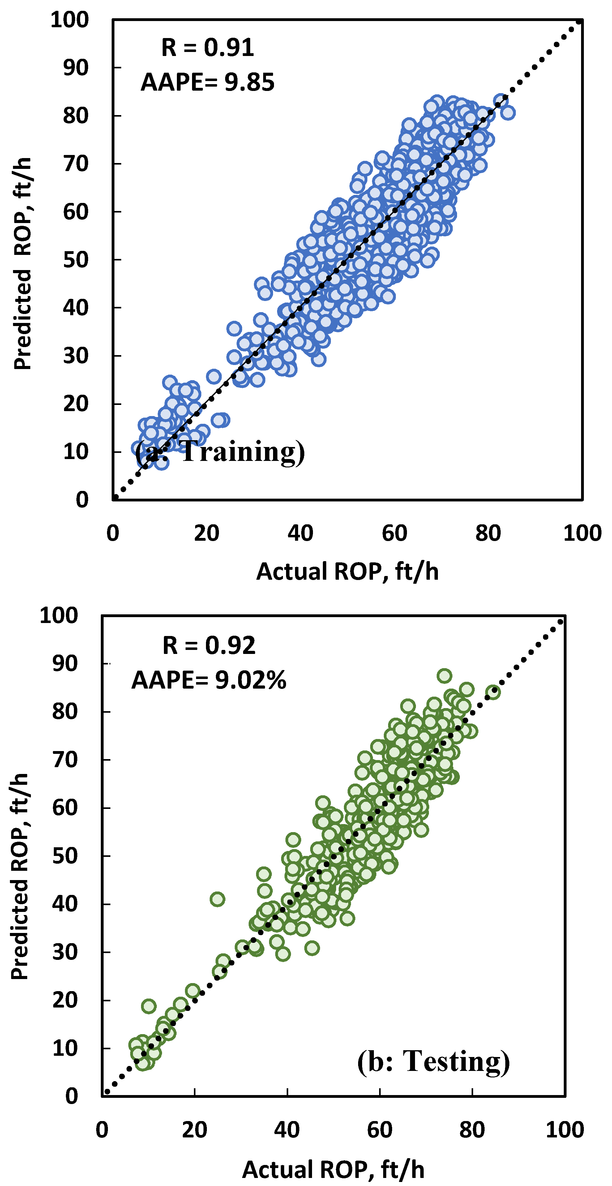
3.1. Model Development and Results
3.2. ANN Model Empirical Correlation
- i-
- Multiplication of the input parameters, x1, x2, x3, ... xn by the associated input weights;
- ii-
- Summation of the weight and input product to the bias value associated with the neuron;
- iii-
- The passage of the summation result, u, through an activation function (linear or nonlinear transformation), Φ. The transfer function can be logistic sigmoid (logsig), hyperbolic tangent sigmoidm (tansig), or linear (purelin), as described in Table 4.
- m: Number of neurons
- n: Number of inputs
- X: The input matrix (x1, x2, …, xn)
- LW: Layer weights matrix, [1, m]
- IW: Input weights matrix, [m, n]
- b1: First layer bias matrix, [m,1]
- b2: Second layer bias, scalar
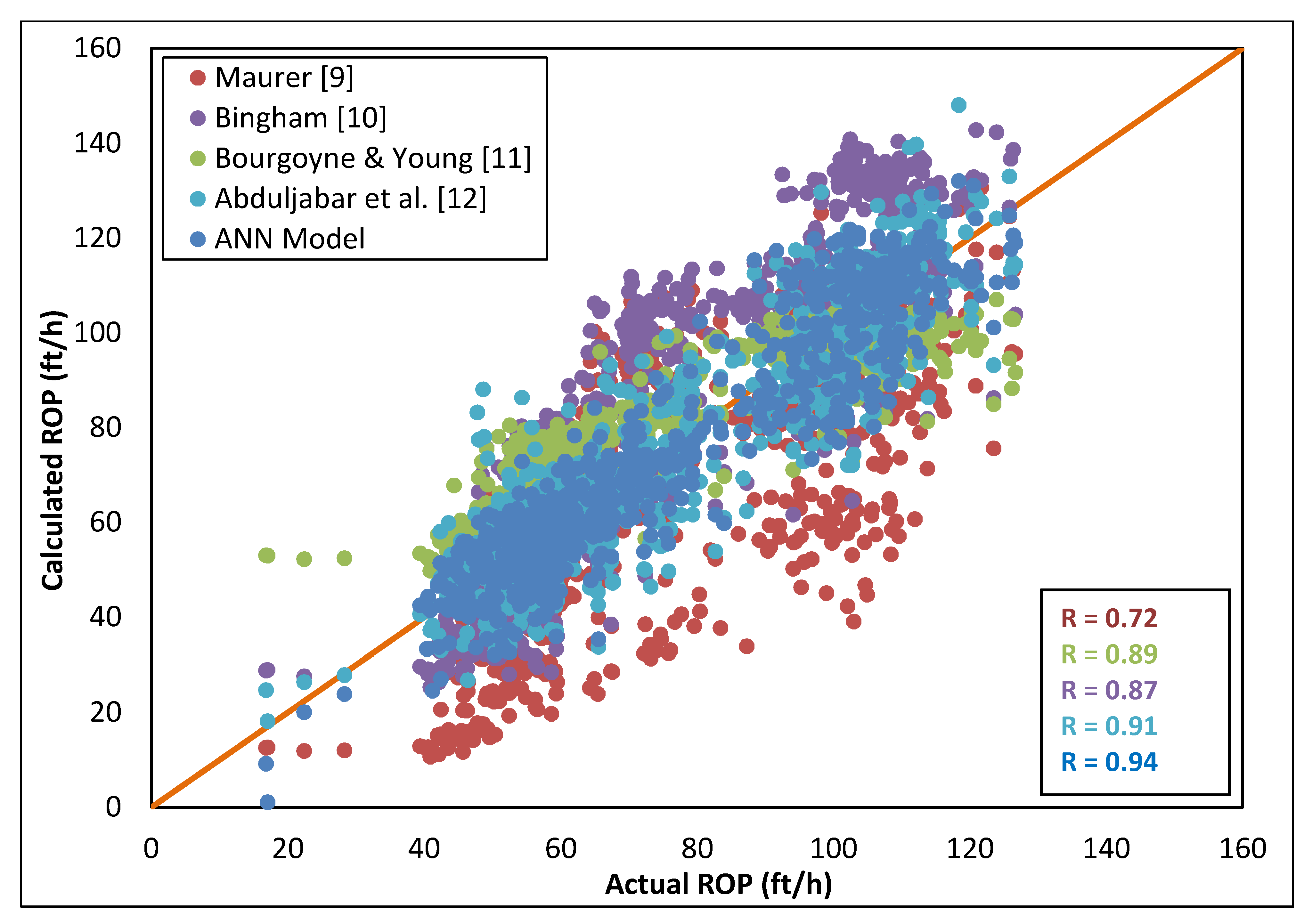
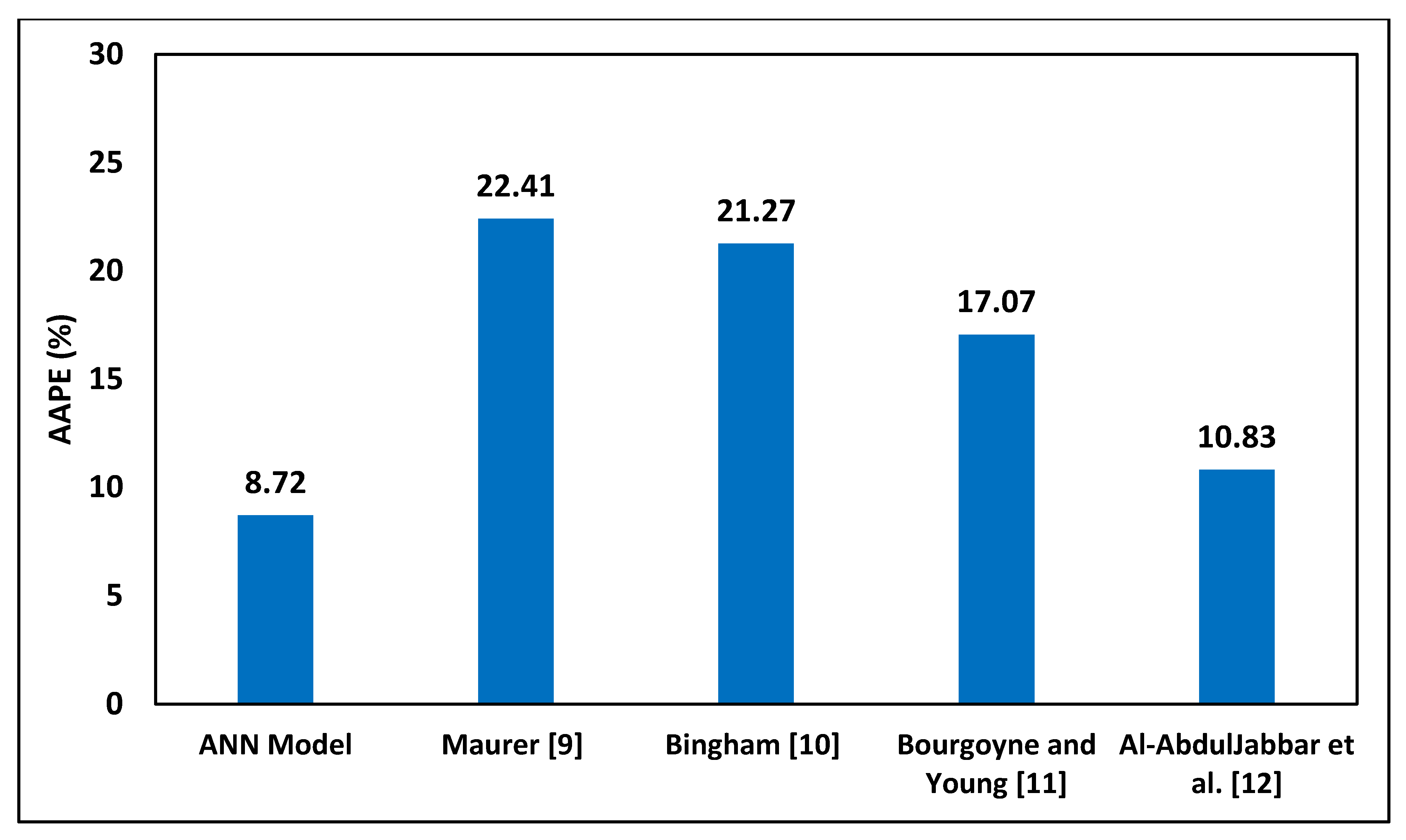
3.3. Model Comparison
4. Conclusions
Author Contributions
Funding
Conflicts of Interest
List of Symbols
| T | Torque, klbf-ft |
| Q | Flow rate, gpm |
| R | Correlation coefficient |
| h | Hour |
| m | Number of neurons |
| n | Number of inputs |
| X | The input matrix |
| LW | Layer weights matrix |
| IW | Input weights matrix |
| b | Bias matrix |
| a | Coefficient |
| c | Constant |
| Φ | Activation function |
List of Abbreviations
| ROP | Rate of penetration, ft/h |
| UCS | Uniaxial compressive strength, psi |
| WOB | Weight on bit, klbf |
| RPM | Revolution per minute |
| AAPE | Average absolute percentage error |
| SPP | Stand pipe pressure, psi |
| ANN | Artificial neural network |
References
- Lukawski, M.Z.; Anderson, B.J.; Augustine, C.; Capuano, L.E.; Beckers, K.F.; Livesay, B.; Tester, J.W. Cost analysis of oil, gas, and geothermal well drilling. J. Pet. Sci. Eng. 2014, 118, 1–14. [Google Scholar] [CrossRef]
- Wardlaw, H. Simplified Analysis Aids in Optimizing Drilling Factors for Minimum Cost. J. Pet. Technol. 1961, 13, 475–482. [Google Scholar] [CrossRef]
- Schreuder, J.; Sharpe, P. Drilling The Limit-A Key To Reduce Well Costs. In Proceedings of the SPE Asia Pacific Improved Oil Recovery Conference, Society of Petroleum Engineers (SPE), Kuala Lumpur, Malaysia, 25–26 October 1999; pp. 25–26. [Google Scholar]
- Judzis, A.; Black, A.D.; Curry, D.A.; Meiners, M.J.; Grant, T.; Bland, R.G. Optimization of Deep-Drilling Performance--Benchmark Testing Drives ROP Improvements for Bits and Drilling Fluids. SPE Drill. Complet. 2009, 24, 25–39. [Google Scholar] [CrossRef]
- He, X.; Halsey, G.; Kyllingstad, A. Interactions between Torque and Helical Buckling in Drilling. In Proceedings of the SPE Annual Technical Conference and Exhibition; Society of Petroleum Engineers (SPE), Dallas, TX, USA, 22–25 October 1995. [Google Scholar]
- Maglione, R.; Robotti, G. Field Rheological Parameters Improve Stand Pipe Pressure Prediction While Drilling. In Proceedings of the SPE Latin America Petroleum Engineering Conference; Society of Petroleum Engineers (SPE), Port-of-Spain, Trinidad, 23–26 April 1996. [Google Scholar]
- Eren, T.; Ozbayoglu, M.E. Real Time Optimization of Drilling Parameters During Drilling Operations. In Proceedings of the SPE Oil & Gas India Conference and Exhibition, Society of Petroleum Engineers (SPE), Mumbai, India, 20–22 January 2010. [Google Scholar]
- Bielstrein, W.J.; Cannon, G.E. Factors Affecting the Rate of Penetration of Bits. American Petroleum Institute; Paper API-50-061 presented at the spring meeting; Southwestern District Division of Production: Dallas, TX, USA, 1950. [Google Scholar]
- Maurer, W. The Perfect-Cleaning Theory of Rotary Drilling. J. Pet. Technol. 1962, 14, 1270–1274. [Google Scholar] [CrossRef]
- Bingham, M.G. A New Approach to Interpreting Rock Drillability; Petroleum Pub. Co.: Houston, TX, USA, 1965. [Google Scholar]
- Bourgoyne, A.; Young, F. A Multiple Regression Approach to Optimal Drilling and Abnormal Pressure Detection. Soc. Pet. Eng. J. 1974, 14, 371–384. [Google Scholar] [CrossRef]
- Al-Abduljabbar, A.; Elkatatny, S.; Mahmoud, M.; AbdelGawad, K.; Al-Majed, A.; Al-Abduljabbar, A.A. Robust Rate of Penetration Model for Carbonate Formation. J. Energy Resour. Technol. 2018, 141, 042903. [Google Scholar] [CrossRef]
- Nakamoto, P. Neural Networks and Deep Learning; CreateSpace Independent Publishing Platform: Scotts Valley, CA, USA, 2017. [Google Scholar]
- Hemphill, T.; Bern, P.A.; Rojas, J.; Ravi, K. Field Validation of Drillpipe Rotation Effects on Equivalent Circulating Density. In Proceedings of the SPE Annual Technical Conference and Exhibition, Society of Petroleum Engineers (SPE), California, CA, USA, 11–14 November 2007. [Google Scholar]
- Carrillo, K.I.A.; Avellan, F.J.; Camacho, G. ECD and Downhole Pressure Monitoring While Drilling at Ecuador Operations. In Proceedings of the Latin American & Caribbean Petroleum Engineering Conference, Society of Petroleum Engineers (SPE), Quito, Ecuador, 18–20 November 2015. [Google Scholar]
- Lippmann, R. An introduction to computing with neural nets. IEEE ASSP Mag. 1987, 4, 4–22. [Google Scholar] [CrossRef]
- Hinton, G.E.; Osindero, S.; Teh, Y.-W. A Fast Learning Algorithm for Deep Belief Nets. Neural Comput. 2006, 18, 1527–1554. [Google Scholar] [CrossRef]
- Rao, S.; Ramamurti, V. A hybrid technique to enhance the performance of recurrent neural networks for time series prediction. In Proceedings of the IEEE International Conference on Neural Networks, Institute of Electrical and Electronics Engineers (IEEE), San Francisco, CA, USA, 28 March–1 April 1993; pp. 52–57. [Google Scholar]
- Niculescu, S.P. Artificial neural networks and genetic algorithms in QSAR. J. Mol. Struct. THEOCHEM 2003, 622, 71–83. [Google Scholar] [CrossRef]
- Mirarab, M.; Arzandeh, A.; Naderi, A.; Fatemeh Mirarab, F.; Ghayyem, M. Annular Pressure Loss while Drilling Prediction with Artificial Neural Network Modeling. Eur. J. Sci. Res. 2013, 95, 272–288. [Google Scholar]
- Naganawa, S.; Sato, R.; Ishikawa, M. Cuttings Transport Simulation Combined With Large-Scale Flow Loop Experiment and LWD Data Enables Appropriate ECD Management and Hole Cleaning Evaluation in Extended-Reach Drilling. In Proceedings of the Abu Dhabi International Petroleum Exhibition & Conference; Society of Petroleum Engineers (SPE), Abu Dhabi, UAE, 10–13 November 2014. [Google Scholar]
- Liew, S.S.; Khalil-Hani, M.; Bakhteri, R. An optimized second order stochastic learning algorithm for neural network training. Neurocomputing 2016, 186, 74–89. [Google Scholar] [CrossRef]
- Al-Bulushi, N.I.; King, P.; Blunt, M.J.; Kraaijveld, M. Artificial neural networks workflow and its application in the petroleum industry. Neural Comput. Appl. 2010, 21, 409–421. [Google Scholar] [CrossRef]
- Weiss, W.W.; Balch, R.S.; Stubbs, B.A. How Artificial Intelligence Methods Can Forecast Oil Production. In Proceedings of the SPE/DOE Improved Oil Recovery Symposium, Tulsa, OK, USA, 13–17 April 2002. [Google Scholar]
- Ma, X.; Liu, Z. Predicting the oil production using the novel multivariate nonlinear model based on Arps decline model and kernel method. Neural Comput. Appl. 2016, 29, 579–591. [Google Scholar] [CrossRef]
- Manshad, A.K.; Rostami, H.; Hosseini, S.M.; Rezaei, H. Application of Artificial Neural Network–Particle Swarm Optimization Algorithm for Prediction of Gas Condensate Dew Point Pressure and Comparison With Gaussian Processes Regression–Particle Swarm Optimization Algorithm. J. Energy Resour. Technol. 2016, 138, 032903. [Google Scholar] [CrossRef]
- Alajmi, M.D.; Mishkhes, A.T.; Al-Shammari, M.J.; Abdulraheem, A. Profiling Downhole Casing Integrity Using Artificial Intelligence. In Proceedings of the SPE Digital Energy Conference and Exhibition, Society of Petroleum Engineers (SPE), Texas, TX, USA, 3–5 March 2015. [Google Scholar]
- Elkatatny, S.; Tariq, Z.; Mahmoud, M. Real time prediction of drilling fluid rheological properties using Artificial Neural Networks visible mathematical model (white box). J. Pet. Sci. Eng. 2016, 146, 1202–1210. [Google Scholar] [CrossRef]
- AbdelGawad, K.; Elkatatny, S.; Mousa, T.; Mahmoud, M.; Patil, S. Real Time Determination of Rheological Properties of Spud Drilling Fluids Using a Hybrid Artificial Intelligence Technique. SPE Kingd. Saudi Arab. Annu. Tech. Symp. Exhib. 2018. [Google Scholar] [CrossRef]
- Agwu, O.E.; Akpabio, J.U.; Alabi, S.B.; Dosunmu, A. Artificial intelligence techniques and their applications in drilling fluid engineering: A review. J. Pet. Sci. Eng. 2018, 167, 300–315. [Google Scholar] [CrossRef]
- Sayadi, A.; Monjezi, M.; Talebi, N.; Khandelwal, M. A comparative study on the application of various artificial neural networks to simultaneous prediction of rock fragmentation and backbreak. J. Rock Mech. Geotech. Eng. 2013, 5, 318–324. [Google Scholar] [CrossRef] [Green Version]
- Mohamad, E.T.; Armaghani, D.J.; Momeni, E.; Yazdavar, A.H.; Ebrahimi, M. Rock strength estimation: A PSO-based BP approach. Neural Comput. Appl. 2016, 30, 1635–1646. [Google Scholar] [CrossRef]
- Elkatatny, S.; Tariq, Z.; Mahmoud, M.; Abdulraheem, A.; Mohamed, I. An integrated approach for estimating static Young’s modulus using artificial intelligence tools. Neural Comput. Appl. 2018, 31, 4123–4135. [Google Scholar] [CrossRef]
- Elkatatny, S.; Tariq, Z.; Mahmoud, M.; Mohamed, I.; Abdulraheem, A. Development of New Mathematical Model for Compressional and Shear Sonic Times from Wireline Log Data Using Artificial Intelligence Neural Networks (White Box). Arab. J. Sci. Eng. 2018, 43, 6375–6389. [Google Scholar] [CrossRef]
- Elkatatny, S.; Mahmoud, M.; Mohamed, I.; Abdulraheem, A. Development of a new correlation to determine the static Young’s modulus. J. Pet. Explor. Prod. Technol. 2017, 8, 17–30. [Google Scholar] [CrossRef] [Green Version]
- Yu, D. Online tool wear prediction in drilling operations using selective artificial neural network ensemble model. Neural Comput. Appl. 2011, 20, 473–485. [Google Scholar] [CrossRef]
- Bhatnagar, A.; Khandelwal, M. An intelligent approach to evaluate drilling performance. Neural Comput. Appl. 2010, 21, 763–770. [Google Scholar] [CrossRef]
- Wang, Y.; Salehi, S. Application of Real-Time Field Data to Optimize Drilling Hydraulics Using Neural Network Approach. J. Energy Resour. Technol. 2015, 137, 062903. [Google Scholar] [CrossRef]
- Ashrafi, S.B.; Anemangely, M.; Sabah, M.; Ameri, M.J. Application of hybrid artificial neural networks for predicting rate of penetration (ROP): A case study from Marun oil field. J. Pet. Sci. Eng. 2019, 175, 604–623. [Google Scholar] [CrossRef]
- Barbosa, L.F.F.M.; Nascimento, A.; Mathias, M.H.; De Carvalho, J.A. Machine learning methods applied to drilling rate of penetration prediction and optimization-A review. J. Pet. Sci. Eng. 2019, 183, 106332. [Google Scholar] [CrossRef]
- Abbas, A.K.; Rushdi, S.; Alsaba, M. Modeling Rate of Penetration for Deviated Wells Using Artificial Neural Network. In Proceedings of the Abu Dhabi International Petroleum Exhibition & Conference; Society of Petroleum Engineers (SPE), Abu Dhabi, UAE, 12–15 November 2018. [Google Scholar]
- Moussa, T.; Elkatatny, S.; Mahmoud, M.; Abdulraheem, A. Development of New Permeability Formulation From Well Log Data Using Artificial Intelligence Approaches. J. Energy Resour. Technol. 2018, 140, 072903. [Google Scholar] [CrossRef]
- Amar, K.; Ibrahim, A. Rate of Penetration Prediction and Optimization using Advances in Artificial Neural Networks, a Comparative Study. In Proceedings of the International Conference on Evolutionary Computation Theory and Applications; SciTePress: Setúbal, Portugal, 2012; pp. 647–652. [Google Scholar]
- Amer, M.M.; Dahab, A.S.; El-Sayed, A.-A.H. An ROP Predictive Model in Nile Delta Area Using Artificial Neural Networks. SPE Kingd. Saudi Arab. Annu. Tech. Symp. Exhib. 2017, 24–27. [Google Scholar] [CrossRef]
- Elkatatny, S. New Approach to Optimize the Rate of Penetration Using Artificial Neural Network. Arab. J. Sci. Eng. 2017, 43, 6297–6304. [Google Scholar] [CrossRef]
- Kamel, M.A.; Elkatatny, S.; Mysorewala, M.; Al-Majed, A.; Elshafei, M. Adaptive and Real-Time Optimal Control of Stick–Slip and Bit Wear in Autonomous Rotary Steerable Drilling. J. Energy Resour. Technol. 2017, 140, 032908. [Google Scholar] [CrossRef]
- Eichie, J.O.; Oyedum, O.D.; Ajewole, M.O.; Aibinu, A. Artificial Neural Network model for the determination of GSM Rxlevel from atmospheric parameters. Eng. Sci. Technol. Int. J. 2017, 20, 795–804. [Google Scholar] [CrossRef] [Green Version]


| Statistical Parameter | ROP (ft/h) | Q (gal/min) | Drill String Rotation Speed (RPM) | SPP (psi) | Torque (Klbf-ft) | WOB (Klbf) | UCS (psi) |
|---|---|---|---|---|---|---|---|
| Minimum | 5.00 | 859.30 | 76.9 | 1396.3 | 7.1 | 31.10 | 1821.1 |
| Maximum | 96.70 | 1110.60 | 157.9 | 2853.1 | 22 | 61.30 | 42,819 |
| Mean | 57.68 | 998.95 | 140.02 | 2291.2 | 16.18 | 48.78 | 13,354 |
| Kurtosis | −0.82 | −1.30 | −1.31 | −0.50 | −1.06 | −0.73 | 1.79 |
| Skewness | 3.42 | 4.02 | 5.84 | 3.28 | 4.34 | 3.54 | 7.34 |
| Statistical Parameter | ROP (ft/h) | Q (gal/min) | Drillstring Rotation Speed (RPM) | SPP (psi) | Torque, (Klbf-ft) | WOB (Klbf) | UCS (psi) |
|---|---|---|---|---|---|---|---|
| Minimum | 5.4 | 807 | 51 | 1357 | 3.8 | 6.5 | 1996.2 |
| Maximum | 153.7 | 1124 | 119 | 3827 | 22.4 | 58 | 28,190 |
| Mean | 106.87 | 1028.6 | 101.86 | 3023 | 15.13 | 40.15 | 11,654 |
| Kurtosis | −0.31 | −1.51 | −2.57 | −0.6695 | −0.31 | −0.03 | 0.97 |
| Skewness | 1.97 | 3.56 | 12.04 | 2.51 | 2.31 | 2.33 | 5.52 |
| Statistical Parameter | ROP (ft/h) | Q, (gal/min) | Drillstring Rotation Speed (RPM) | SPP (psi) | Torque (Klbf-ft) | WOB (Klbf) | UCS (psi) |
|---|---|---|---|---|---|---|---|
| Minimum | 16.79 | 697.64 | 64.52 | 676.17 | 12.90 | 26.17 | 5087.20 |
| Maximum | 126.66 | 1171.40 | 168.86 | 2628.60 | 23.29 | 58.33 | 28,190 |
| Mean | 72.98 | 890.46 | 129.22 | 1664.40 | 18.25 | 45.19 | 11,382 |
| Kurtosis | 0.59 | 0.33 | −0.20 | 0.44 | 0.80 | −0.51 | 1.30 |
| Skewness | 2.07 | 1.26 | 2.97 | 1.95 | 3.20 | 2.55 | 7.77 |
| Transfer Functions | Definition |
|---|---|
| logsig | |
| tansig | |
| purelin |
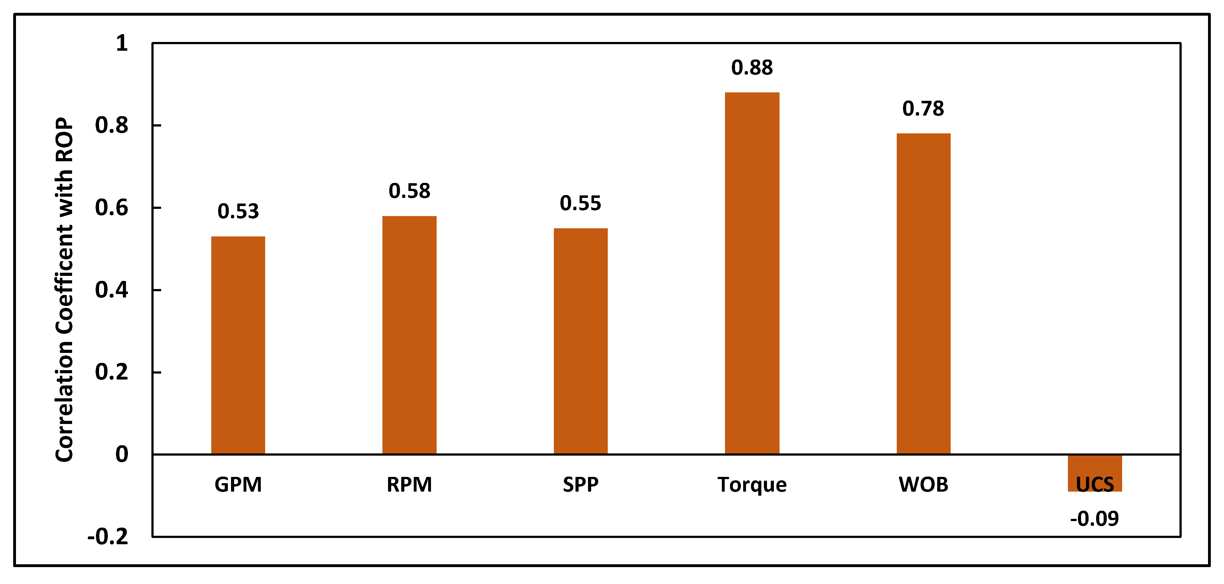
| 0.04535 | 0.28979 | 0.09246 | 0.17677 | 0.73647 | 0.09868 | −0.06879 |
© 2020 by the authors. Licensee MDPI, Basel, Switzerland. This article is an open access article distributed under the terms and conditions of the Creative Commons Attribution (CC BY) license (http://creativecommons.org/licenses/by/4.0/).
Share and Cite
Elkatatny, S.; Al-AbdulJabbar, A.; Abdelgawad, K. A New Model for Predicting Rate of Penetration Using an Artificial Neural Network. Sensors 2020, 20, 2058. https://doi.org/10.3390/s20072058
Elkatatny S, Al-AbdulJabbar A, Abdelgawad K. A New Model for Predicting Rate of Penetration Using an Artificial Neural Network. Sensors. 2020; 20(7):2058. https://doi.org/10.3390/s20072058
Chicago/Turabian StyleElkatatny, Salaheldin, Ahmed Al-AbdulJabbar, and Khaled Abdelgawad. 2020. "A New Model for Predicting Rate of Penetration Using an Artificial Neural Network" Sensors 20, no. 7: 2058. https://doi.org/10.3390/s20072058