Characterization of the Observational Covariance Matrix of Hyper-Spectral Infrared Satellite Sensors Directly from Measured Earth Views


Abstract
:
1. Introduction
2. Data and Methods
2.1. Data
2.2. Methods
3. Results
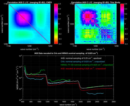
3.1. IASI
- Cloudy tropical set: This consists of 14,321 spectra selected in the tropical belt (−35° to 35° latitude) with a cloud fraction %.
- Clear tropical set: This consists of 9324 spectra selected in the tropical belt (−35° to 35° latitude) with a cloud fraction %.
- Clear High-Latitude set: This consists of 11,230 spectra selected at latitude (north and south) higher than 60° with a cloud fraction %.
3.2. CrIS
3.3. HIRAS
4. Discussion
Author Contributions
Funding
Acknowledgments
Conflicts of Interest
Abbreviations
| CMA | China Meteorological Administration |
| CNES | Centre National d’Etudes Spatiales |
| CrIS | Cross-track Infrared Sounder |
| DS | Deep Space, cold blackbody source |
| EPS | European Polar System |
| EUMETSAT | European Organization for the Exploitation of Meteorological Satellite |
| FOR | Field of Regard |
| FSR | Full Spectral Resolution |
| HIRAS | Hyper-spectral Infrared Atmospheric Sounder |
| IASI | Infrared Atmospheric Sounder Interferometer |
| ICT | Internal Calibration Target, warm blackbody source |
| IFOV | Instantaneous Field of View |
| LWIR | Long Wave InfraRed |
| Metop | Meteorological Operational platform |
| MPD | Maximum Path Difference |
| MWIR | Mid Wave InfraRed |
| NEDN | Noise Equivalent Difference Radiance |
| NSMC | National Satellite Meteorological Center |
| NSR | Normal Spectral Resolution |
| SWIR | Short Wave InfraRed |
References
- Amato, A.; De Canditiis, D.; Serio, C. Effect of apodization on the retrieval of geophysical parameters from Fourier-transform spectrometers. Appl. Opt. 1998, 37, 6537–6543. [Google Scholar] [CrossRef] [PubMed]
- Zavyalov, V.; Esplin, M.; Scott, D.; Esplin, B.; Bingham, G.; Hoffman, E.; Lietzke, C.; Predina, J.; Frain, R.; Suwinski, L.; et al. Noise performance of the CrIS instrument. J. Geophys. Res. Atmos. 2013, 118, 13108–13120. [Google Scholar] [CrossRef] [Green Version]
- Serio, C.; Standfuss, C.; Masiello, G.; Liuzzi, G.; Dufour, R.E.; Tournier, B.; Stuhlmann, R.; Tjemkes, S.; Antonelli, P. Infrared atmospheric sounder interferometer radiometric noise assessment from spectral residuals. Appl. Opt. 2015, 54, 5924–5936. [Google Scholar] [CrossRef] [PubMed]
- Serio, C.; Masiello, G.; Camy-Peyret, C.; Jacquette, E.; Vandermarcq, O.; Bermudo, F.; Coppens, D.; Tobin, D. PCA determination of the radiometric noise of high spectral resolution infrared observations from spectral residuals: Application to IASI. J. Quant. Spectrosc. Radiat. Transf. 2018, 206, 8–21. [Google Scholar] [CrossRef]
- Amato, U.; Masiello, G.; Serio, C.; Viggiano, M. The σ-IASI code for the calculation of infrared atmospheric radiance and its derivatives. Environ. Model. Softw. 2002, 17, 651–667. [Google Scholar] [CrossRef]
- Carissimo, A.; De Feis, I.; Serio, C. The physical retrieval methodology for IASI: the δ-IASI code. Environ. Model. Softw. 2005, 20, 1111–1126. [Google Scholar] [CrossRef]
- Jolliffe, I.T. Principal Component Analysis; Springer: New York, NY, USA, 2002. [Google Scholar]
- Masiello, G.; Serio, C. Dimensionality-reduction approach to the thermal radiative transfer equation inverse problem. Geophys. Res. Lett. 2004, 31, L11105. [Google Scholar] [CrossRef]
- Liu, X.; Smith, W.L.; Zhou, D.K.; Larar, A. Principal component-based radiative transfer model for hyper-spectral sensors: Theoretical concept. Appl. Opt. 2006, 45, 201–209. [Google Scholar] [CrossRef] [PubMed]
- Liu, X.; Zhou, D.K.; Larar, A.; Smith, W.L.; Mango, S.A. Case-study of a principal-component-based radiative trasnsfer frorward model and retrieval algorithm using EQUATE data. Q. J. R. Meteorol. Soc. 2007, 133, 243–256. [Google Scholar] [CrossRef]
- Amato, U.; Antoniadis, A.; De Feis, I.; Masiello, G.; Matricardi, M.; Serio, C. Technical Note: Functional sliced inverse regression to infer temperature, water vapour and ozone from IASI data. Atmos. Chem. Phys. 2009, 9, 5321–5330. [Google Scholar] [CrossRef] [Green Version]
- Grieco, G.; Masiello, G.; Serio, C. Interferometric vs Spectral IASI Radiances: Effective Data-Reduction Approaches for the satellite Sounding of Atmospheric Thermodynamical Parameters. Remote Sens. 2010, 2, 2323–2346. [Google Scholar] [CrossRef] [Green Version]
- Collard, A.D.; McNally, A.P.; Hilton, F.I.; Healy, S.B.; Atkinson, N.C. The use of principal component analysis for the assimilation of high-resolution infrared sounder observations for numerical weather prediction. Q. J. R. Meteorol. Soc. 2010, 136, 2038–2050. [Google Scholar] [CrossRef]
- Masiello, G.; Matricardi, M.; Serio, C. The use of IASI data to identify systematic errors in the ECMWF temperature analysis in the upper stratosphere. Atmos. Chem. Phys. 2011, 11, 1009–1021. [Google Scholar] [CrossRef] [Green Version]
- Masiello, G.; Serio, C.; Antonelli, P. Inversion for atmospheric thermodynamical parameters of IASI data in the principal components space. Q. J. R. Meteor. Soc. 2012, 138, 103–117. [Google Scholar] [CrossRef] [Green Version]
- Lee, L.; Zhang, P.; Qi, C.; Hu, X.; Gu, M. HIRAS noise performance improvement based on principal component analysis. Appl. Opt. 2019, 58, 5506–5515. [Google Scholar] [CrossRef] [PubMed]
- Han, Y.; Suwinski, L.; Tobin, D.; Chen, Y. Effect of self-apodization correction on Cross-track Infrared Sounder radiance noise. Appl. Opt. 2015, 54, 10114–10122. [Google Scholar] [CrossRef]
- Schwarz, G. Estimating the dimension of a model. Ann. Statist. 1978, 6, 461–464. [Google Scholar] [CrossRef]
- Hilton, F.; Armante, R.; August, T.; Barnet, C.; Bouchard, A.; Camy-Peyret, C.; Capelle, V.; Clarisse, L.; Clerbaux, C.; Coheur, P.; et al. Hyperspectral Earth Observation from IASI: Five Years of Accomplishments. Bull. Am. Meteorol. Soc. 2012, 93, 347–370. [Google Scholar] [CrossRef]
- Chinaud, J.; Jacquette, E.; Le Barbier, L. Covariance Matrix; Technical Note, IA-TN-0000-3274-CNE; CNES: Toulouse, France, 2018.
- Lu, Q.; Wu, C.; Qi, C.; Feng, X.; Liu, H.; Xiao, X. Brief Introduction of the Hyper-Spectral Infrared Sounder from FY-4A and FY-3D. Available online: https://www.ecmwf.int/node/17228 (accessed on 1 March 2020).
- Anderson, T.W. An Introduction to Multivariate Statistical Analysis, 3rd ed.; J. Wiley&Sons: Hoboken, NJ, USA, 2009. [Google Scholar]
- Jacquette, E.; Chinaud, J. IASI Quarterly Performance Report from 2012/09/01 to 2012/11/30 by IASI TEC (Technical Expertise Center) for IASI PFM-R on METOP A; CNES: Tolouse, France, 2013.
- Masiello, G.; Serio, C.; Shimoda, H. Qualifying IMG tropical spectra for clear sky. J. Quant. Spectrosc. Radiat. Transf. 2003, 77, 131–148. [Google Scholar] [CrossRef]
- Amato, U.; Lavanant, L.; Liuzzi, G.; Masiello, G.; Serio, C.; Stuhlmann, R.; Tjemkes, S.A. Cloud mask via cumulative discriminant analysis applied to satellite infrared observations: Scientific basis and initial evaluation. Atmos. Meas. Tech. 2014, 7, 3355–3372. [Google Scholar] [CrossRef]


| Characteristic | Value | Units |
|---|---|---|
| Spectral Coverage | 645 to 2760 | cm |
| Number of Bands | 3 | |
| Spectral Coverage Band 1 | 645 to 1210 | cm |
| Spectral Coverage Band 2 | 1210 to 2000 | cm |
| Spectral Coverage Band 3 | 2000 to 2760 | cm |
| Scan Type | Step and Stare | |
| Scan Rate | 8 | s |
| Stare Interval | 151 | ms |
| Step Interval | 8/37 | s |
| Pixels for Field of Regard (FOR) | ||
| Swath | degrees | |
| Swath width | km | |
| Number of FOR per Swath width | 30 | |
| Single Pixel or Instantaneous Field of View (IFOV) shape at nadir | circular | |
| IFOV size at nadir | 12 | km |
| IFOV size at edge of scan line across track | 39 | km |
| IFOV size at edge of scan line along track | 20 | km |
| Characteristic | Value | Units |
|---|---|---|
| Spectral Coverage | 648.75 to 2555 | cm |
| Number of Bands | 3 | |
| Spectral Coverage Band 1 | 648.75 to 1096.25 | cm |
| Spectral Coverage Band 2 | 1207.50 to 1752.50 | cm |
| Spectral Coverage Band 3 | 2150 to 2555 | cm |
| Scan Type | Step and Stare | |
| Scan Rate | 8 | s |
| Pixels for Field of Regard (FOR) | ||
| Swath | ±50 | degrees |
| Swath width | km | |
| Number of FOR per Swath width | 30 | |
| Single Pixel or Instantaneous Field of View (IFOV) shape at nadir | circular | |
| IFOV size at nadir | 14 | km |
| Data Set | No. Spectra | ||||
|---|---|---|---|---|---|
| Band 1 | Band 2 | Band 3 | |||
| IASI | |||||
| Tropical CF = 100% | 298 | 14,321 | |||
| Tropical CF ≤ 5% | 185 | 9324 | |||
| High Latitude CF ≤ 5% | 276 | 11,230 | |||
| Tropical all sky | Pixel 1 | 253 | 10,240 | ||
| Pixel 2 | 288 | 10,240 | |||
| Pixel 3 | 230 | 10,240 | |||
| Pixel 4 | 225 | 10,240 | |||
| CrIS | |||||
| September 2015 | 95 | 75 | 20 | 10,080 | |
| November 2015 | 89 | 78 | 22 | 9360 | |
| HIRAS | |||||
| July 2019 | 93 | 83 | 34 | 8320 | |
© 2020 by the authors. Licensee MDPI, Basel, Switzerland. This article is an open access article distributed under the terms and conditions of the Creative Commons Attribution (CC BY) license (http://creativecommons.org/licenses/by/4.0/).
Share and Cite
Serio, C.; Masiello, G.; Mastro, P.; Tobin, D.C. Characterization of the Observational Covariance Matrix of Hyper-Spectral Infrared Satellite Sensors Directly from Measured Earth Views. Sensors 2020, 20, 1492. https://doi.org/10.3390/s20051492
Serio C, Masiello G, Mastro P, Tobin DC. Characterization of the Observational Covariance Matrix of Hyper-Spectral Infrared Satellite Sensors Directly from Measured Earth Views. Sensors. 2020; 20(5):1492. https://doi.org/10.3390/s20051492
Chicago/Turabian StyleSerio, Carmine, Guido Masiello, Pietro Mastro, and David C. Tobin. 2020. "Characterization of the Observational Covariance Matrix of Hyper-Spectral Infrared Satellite Sensors Directly from Measured Earth Views" Sensors 20, no. 5: 1492. https://doi.org/10.3390/s20051492