Coherent Markov Random Field-Based Unreliable DSM Areas Segmentation and Hierarchical Adaptive Surface Fitting for InSAR DEM Reconstruction


Abstract
:1. Introduction
- (1)
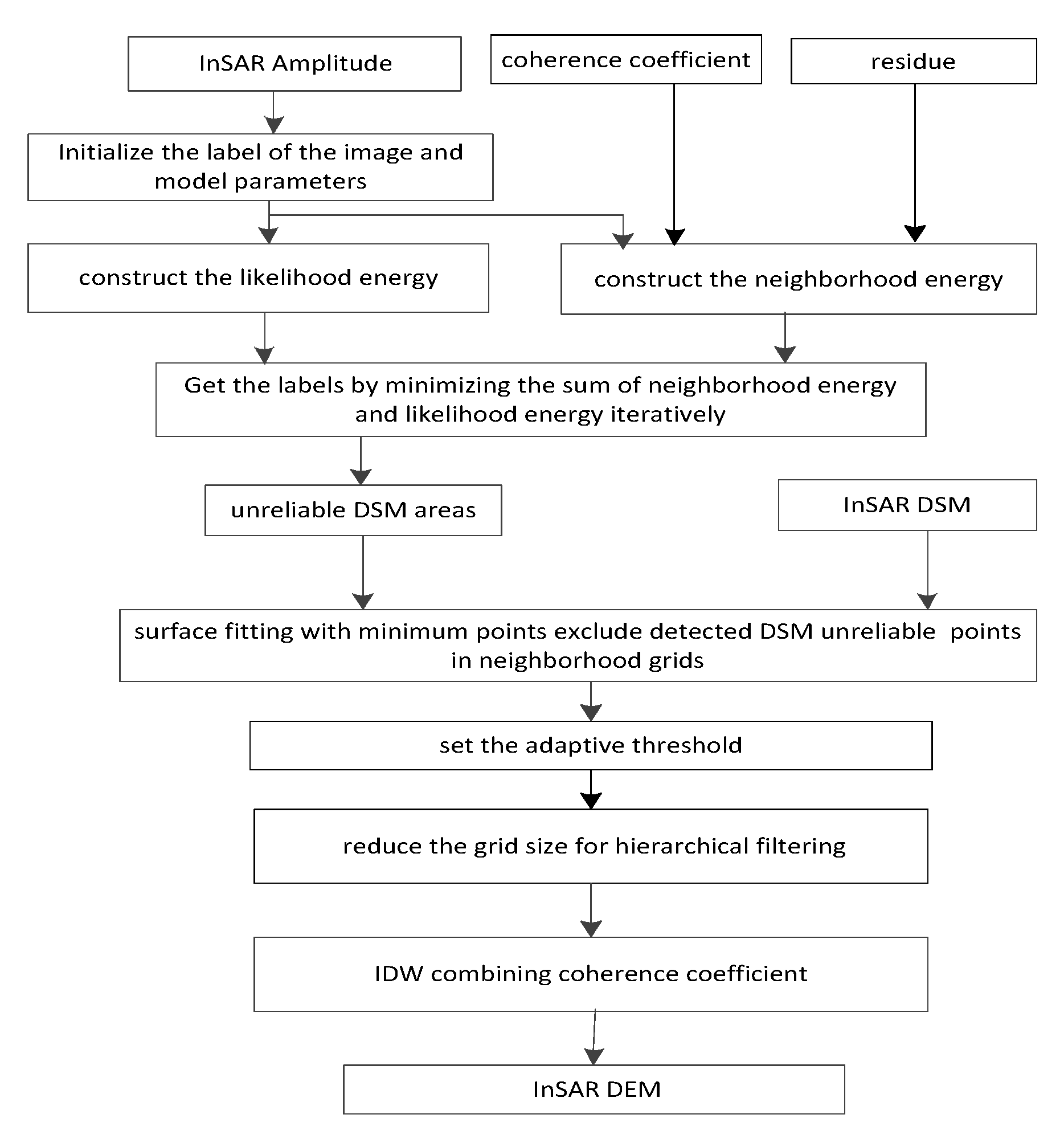
- In order to avoid the influence of the extreme points in the unreliable DSM areas when performing DEM reconstruction, segmentation based on the intensity of pixel gray levels in the InSAR amplitude image (which is helpful for the selection of ground points) was firstly used to identify the unreliable DSM areas for improving the performance of the subsequent DEM reconstruction.
- (2)
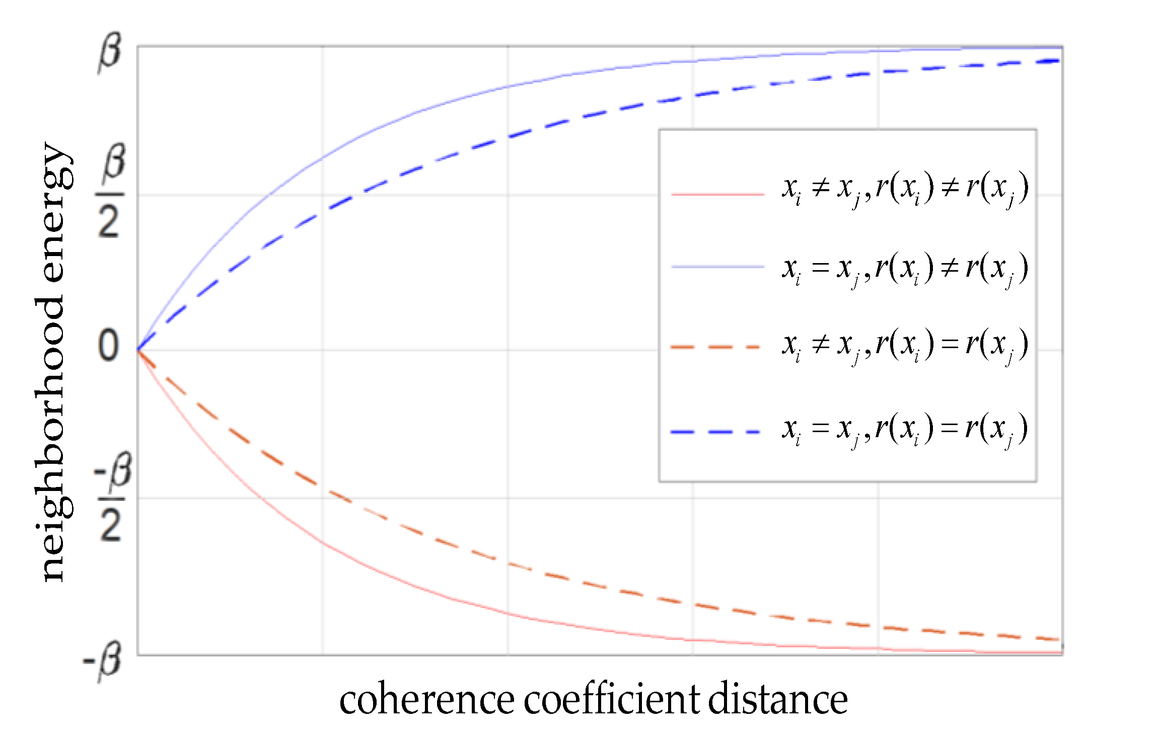
- In order to improve the segmentation performance, we considered the potential of InSAR data information, such that this paper combined the coherence coefficient and residue information of interferometric phase with the neighborhood energy of the MRF, and the full use of contextual relationship was achieved by using the interferometric information between neighboring pixels.
- (3)
- In the general surface fitting-based method, the fixed grid size and threshold will affect the filtering accuracy. Therefore, a new idea of progressively reducing the grid size and setting the adaptive threshold is proposed. It can realize the step-by-step filtering of ground points and the preservation of terrain detail information. At the same time, inverse distance weighted (IDW) interpolation with coherence coefficient is performed for completing the reconstruction of the DEM.
2. Proposed Method
2.1. Unreliable DSM Areas Segmentation with Coherent Markov Random Field (CMRF) Method
2.1.1. Image Segmentation Based on a MRF Model
- (1)
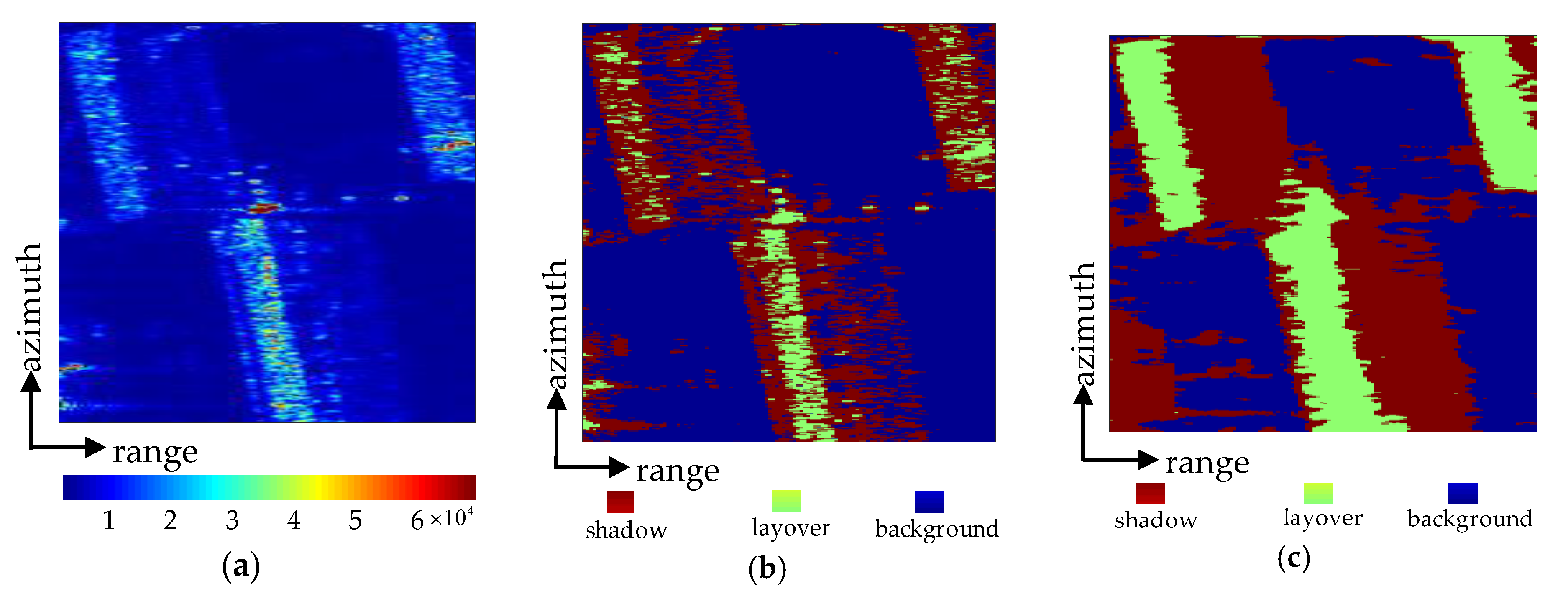
- Layover areas: The characteristics of this area are scattered signals of targets at different positions overlapping at the same distance resolution unit, causing high brightness in the SAR image.
- (2)
- Shadow areas: This area is characterized by an extremely low backscattered signal strength, which is caused by steep terrain or occlusion by towering targets.
- (3)
- Background areas: The other areas which don’t belong to the layover or shadow in the scene are grouped into the background, which mainly includes roofs, trees, and bare ground.
2.1.2. CMRF Segmentation
2.2. DEM Reconstruction Based on Hierarchical Adaptive Surface Fitting
2.2.1. Reconstruction Method Based on Surface Fitting
2.2.2. Hierarchical Adaptive Surface Fitting
- (1)
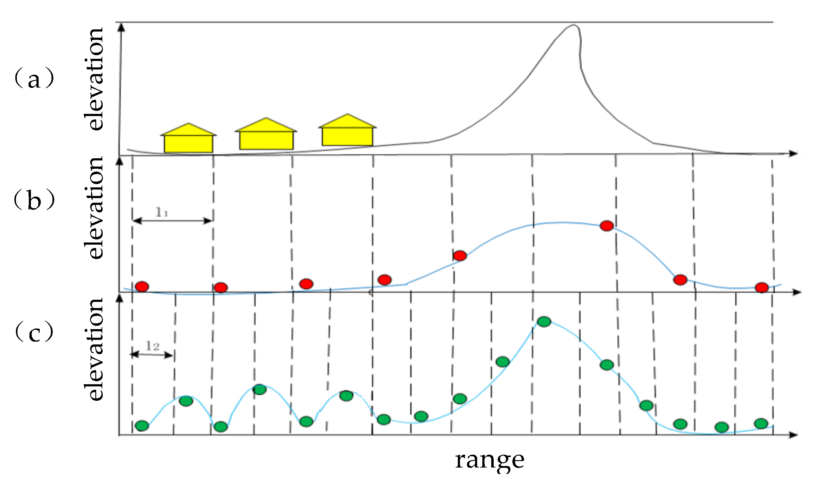
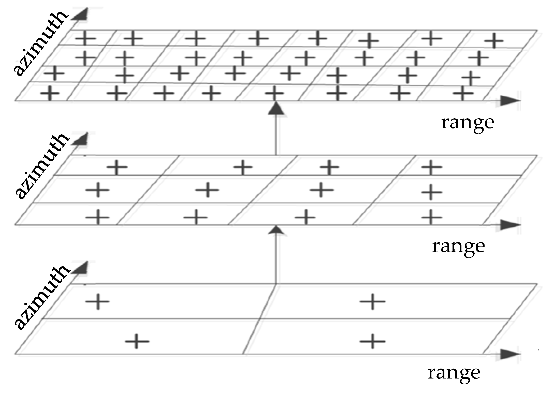
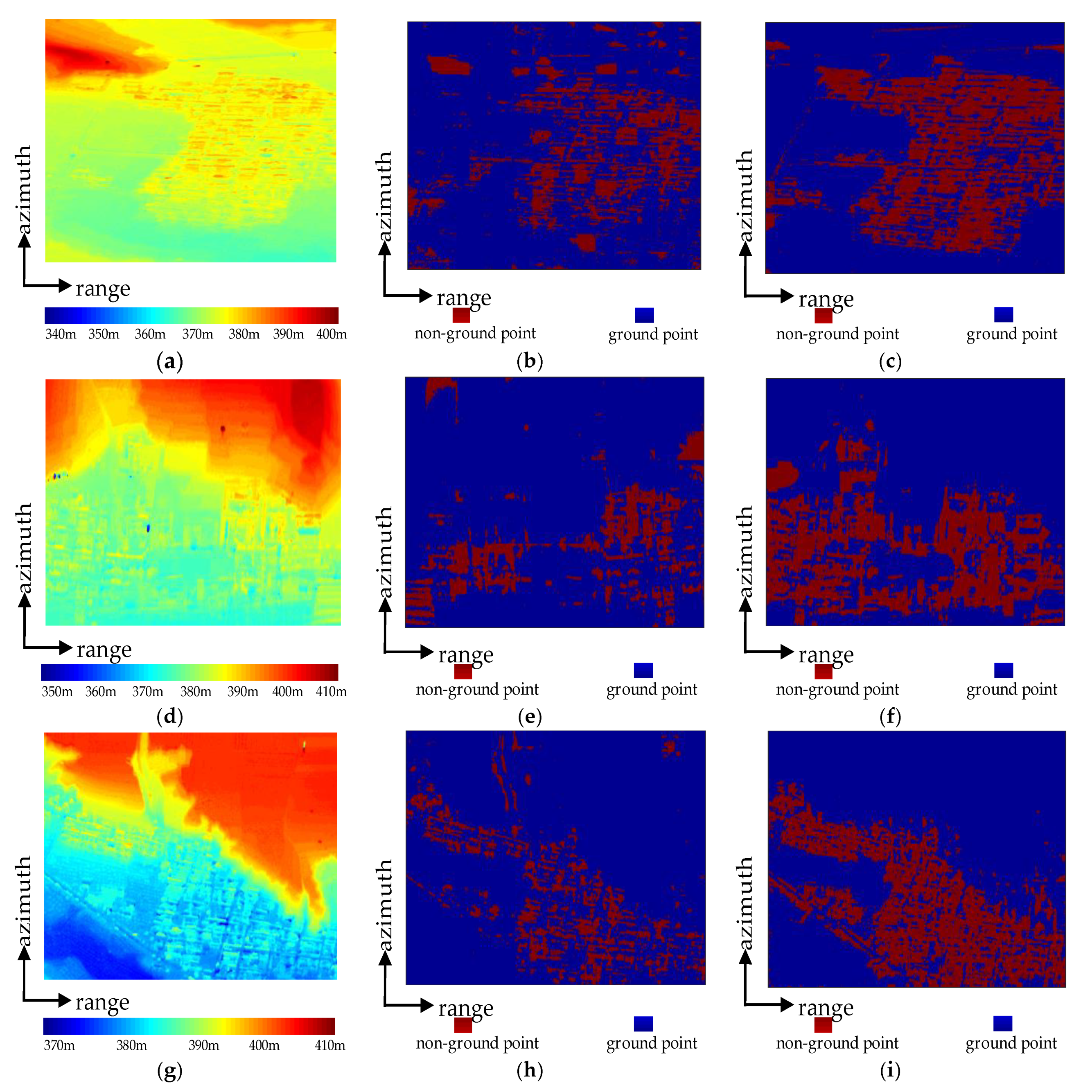
- Hierarchical surface fitting: In the first iteration, the DSM data is first divided evenly by relatively large-sized grids, and then the minimum elevation points in each grid that are not the unreliable DSM areas are used as candidate ground points. The candidate ground points are compared with the surface obtained by fitting the candidate ground points in the 3 × 3 neighborhood grids. If the difference between the elevation of the candidate ground point and the fitted surface is greater than the threshold, the candidate point will be marked as non-ground points. Due to the large mesh size in the first iteration, it cannot represent the true topographic relief well, and the threshold should be set relatively loosely, filtering out buildings with large elevation values. In order to further locate potential non-ground points, we continuously reduce the size of the mesh and repeated the above steps until the mesh size is less than the preset minimum. Figure 4 shows a schematic diagram of the hierarchical surface fitting process.
- (2)
- Determination of adaptive threshold: As mentioned above, considering the influence of grid size and elevation variance, this paper proposed a method for adaptively determining the threshold, which is shown in the Equation (20). The basic idea is that smaller grid size and variance of elevation difference usually correspond to a more reliable fitting result, which means that the threshold should be relatively strict. Conversely, with the increase of grid size and variance, its ability to represent real terrain is weakened, indicating that the fitted terrain has large deviations and the threshold should be relatively loose.where represents the grid size; and represents the variance of elevation difference. and represent the weights of the grid size and variance of elevation difference, respectively.
- (3)
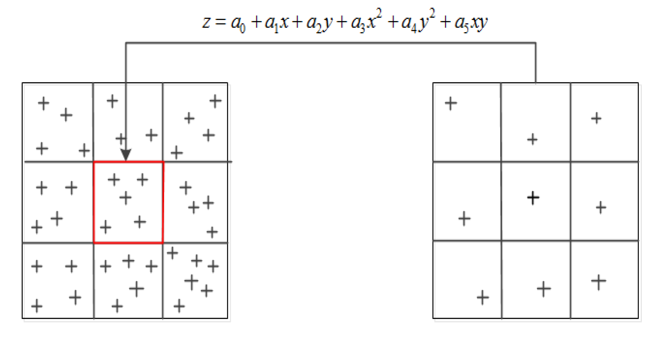
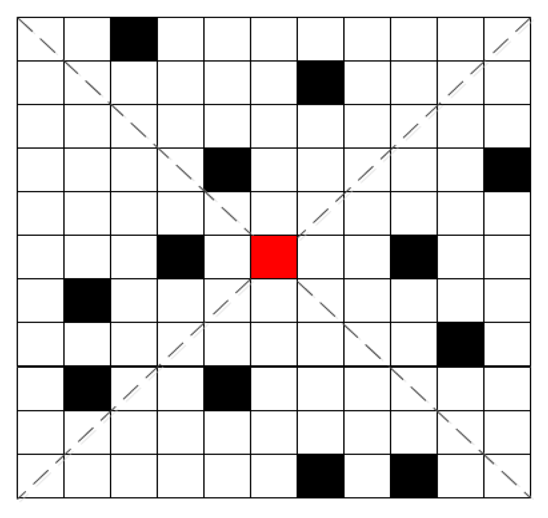
- Interpolation with Coherence-Coefficient-Based IDW: After the ground points have been acquired by hierarchical surface fitting, the next step is to perform the interpolation with discrete ground points. In this study, the IDW algorithm was selected to interpolate the ground DEM, and it determines the weighting coefficient of ground points based on the distance between the known ground point and the interpolation point. This algorithm searches for ground points within the initial area, and if the number of ground points meets the set threshold, the search is stopped and then the weight of the searched ground points is calculated and interpolation is performed; otherwise the search radius is increased and the search is continued until the condition is satisfied. Figure 5 shows the algorithm execution diagram. When calculating the elevation of the red box, which is the point to be interpolated, search for ground points around it. If the number of black boxes representing the ground points reaches the set threshold, the distance between each ground point and the point to be interpolated is calculated, and then the weight is obtained by Equation (21).where is the distance between the ground point and the point to be interpolated; and is the number of points participating in the calculation. Finally, the product of the weight and the elevation of ground point is summed to obtain the elevation of the point to be interpolated.
3. Results
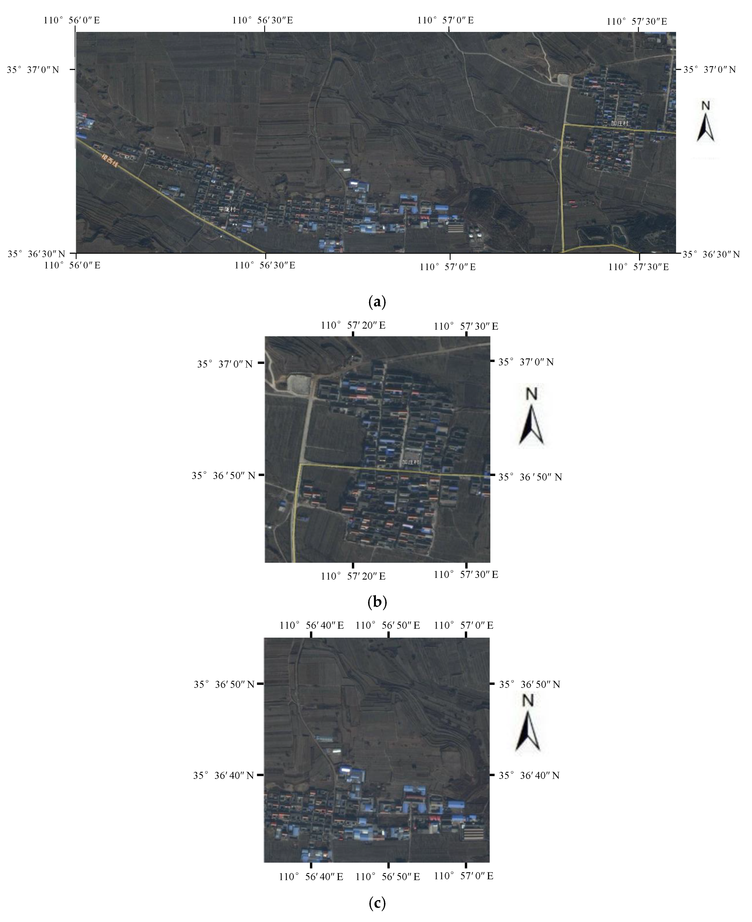
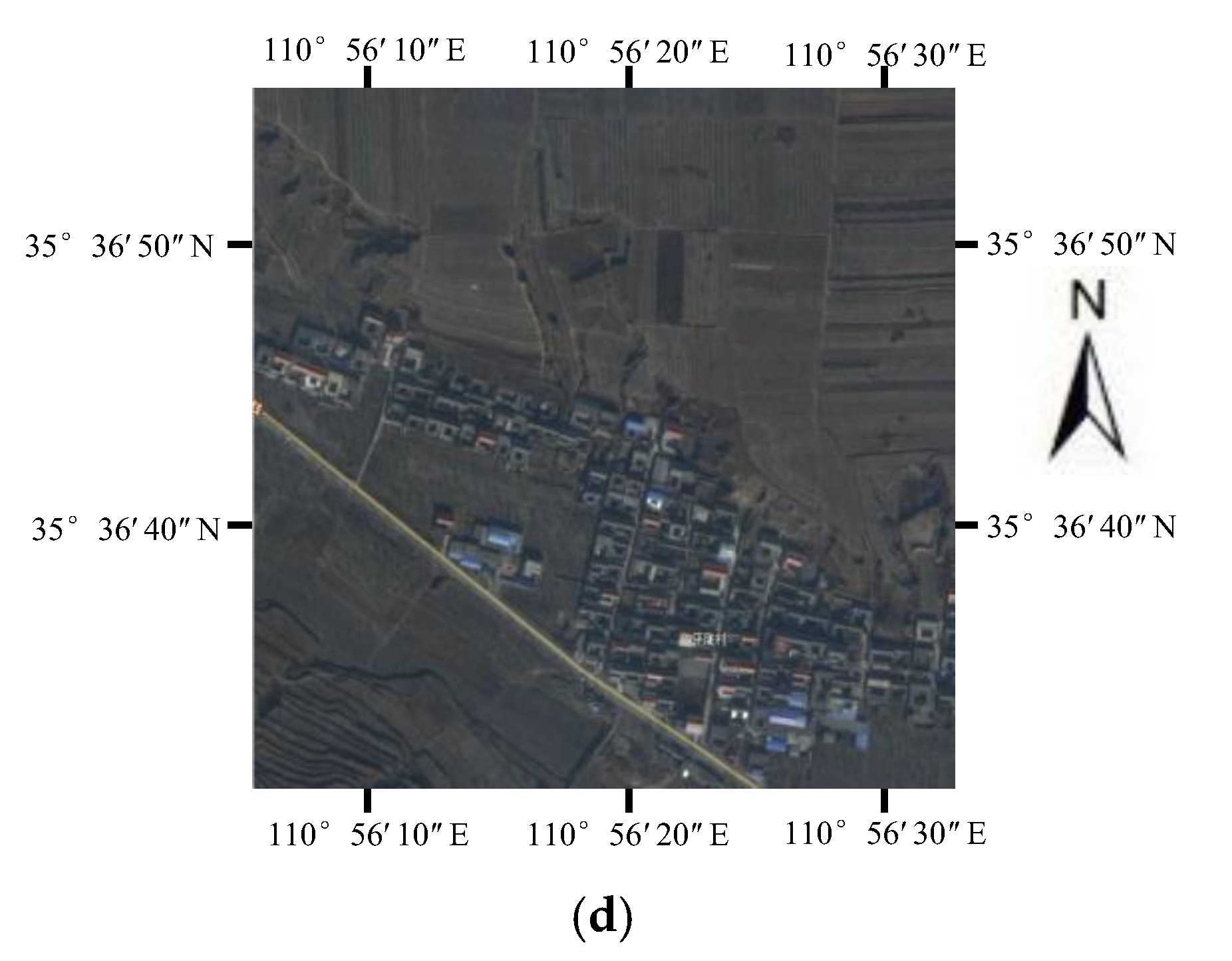
3.1. Testing Data
3.2. The Segmentation Result of CMRF-Based Unreliable DSM Areas
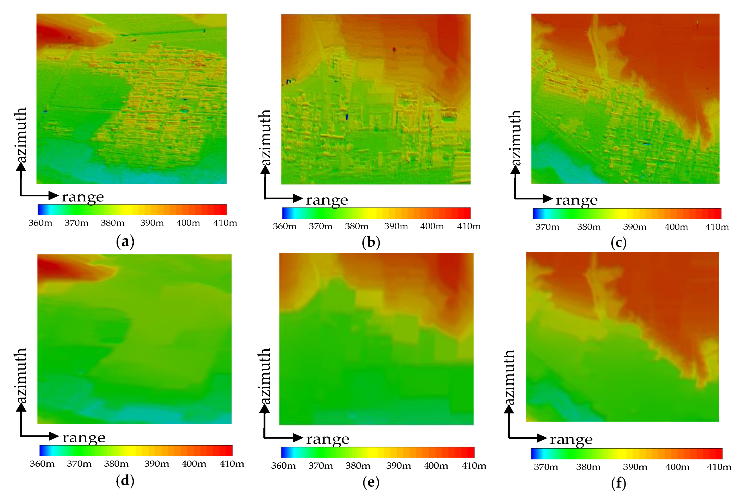
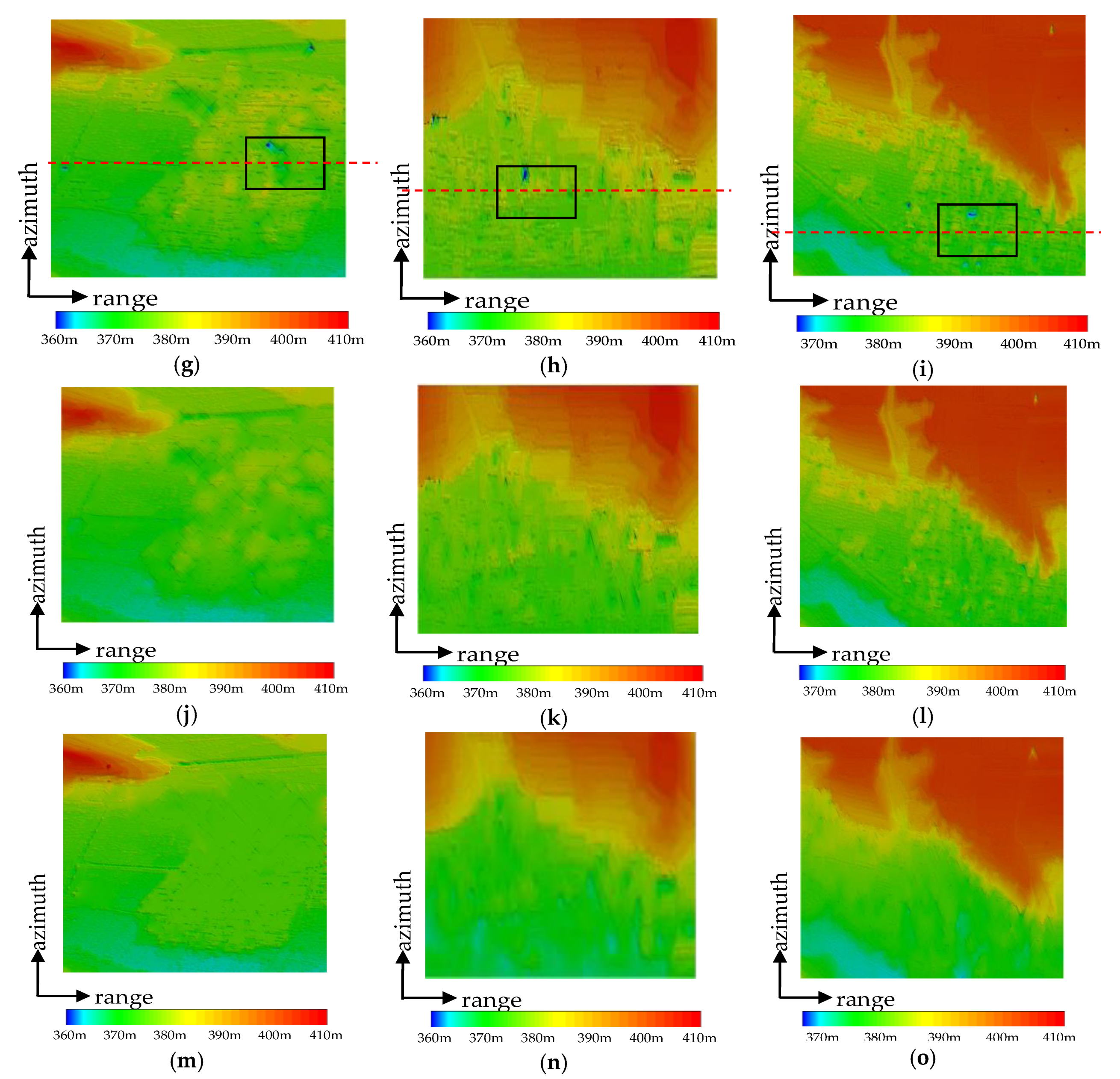
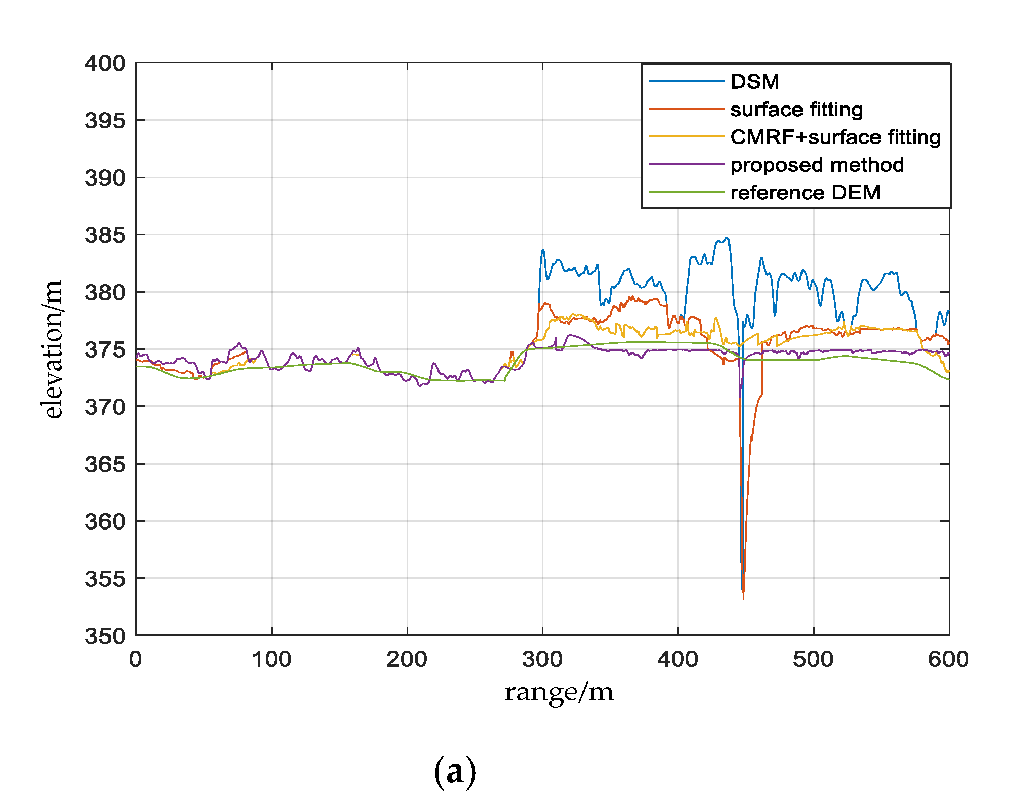
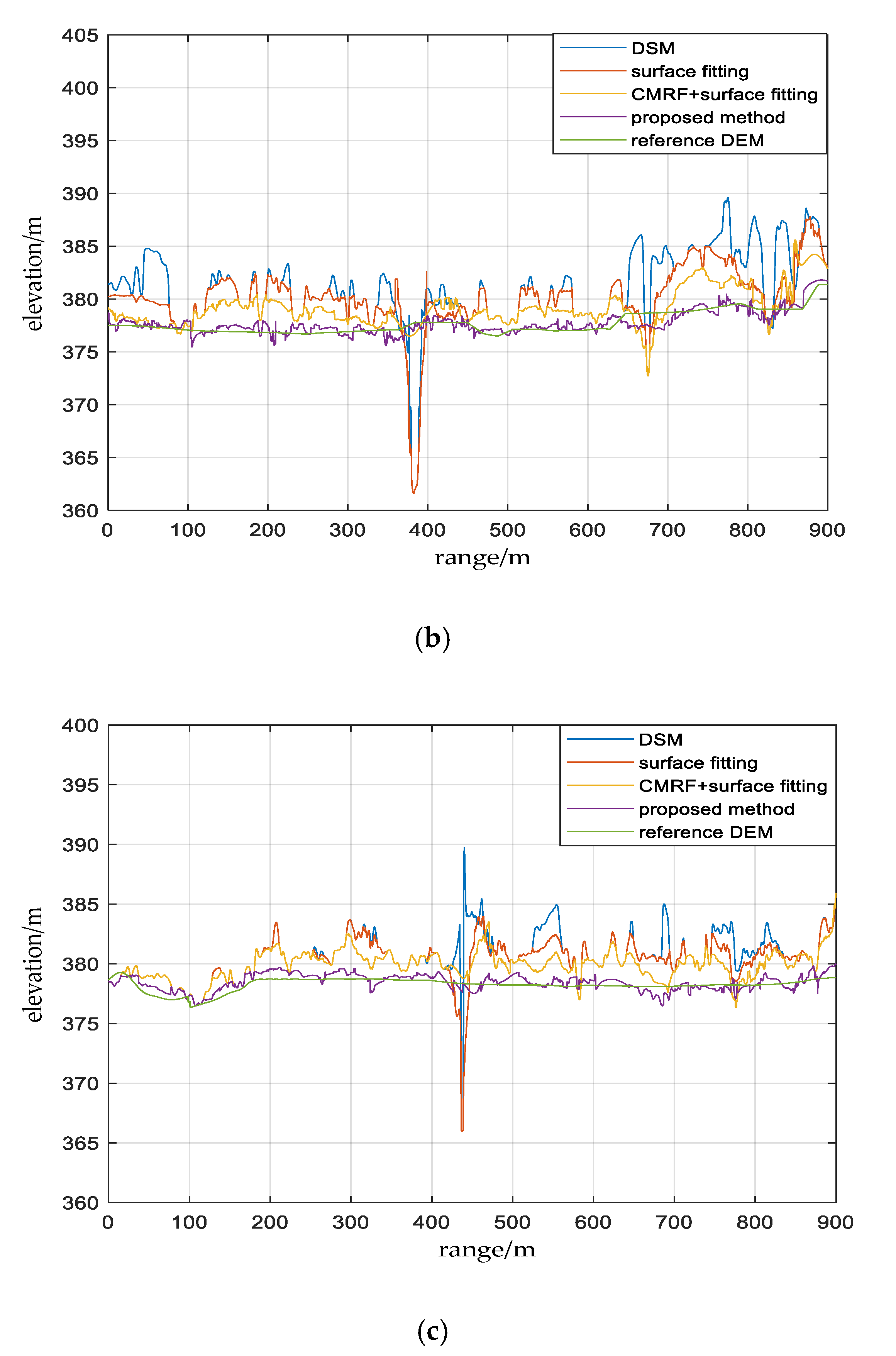
3.3. The DEM Reconstruction Result
3.4. Quantitative Evaluation
4. Conclusions
Author Contributions
Funding
Conflicts of Interest
References
- Perko, R.; Raggam, H.; Gutjahr, K.H.; Schardt, M. Advanced DTM generation from very high resolution satellite stereo images. In Proceedings of the PIA15+HRIGI15—Joint ISPRS Conference 2015, Munich, Germany, 25–27 March 2015; pp. 165–172. [Google Scholar]
- Debella-Gilo, M. Bare-earth extraction and DTM generation from photogrammetric point clouds including the use of an existing lower-resolution DTM. Int. J. Remote Sens. 2015, 37, 3104–3124. [Google Scholar] [CrossRef]
- Zhang, K.; Chen, S.C. A progressive morphological filter for removing nonground measurements from airborne lidar data. IEEE Trans. Geosci. Remote Sens. 2003, 41, 872–882. [Google Scholar] [CrossRef] [Green Version]
- Zhao, X.; Guo, Q.; Su, Y.; Xue, B. Improved progressive TIN densification filtering algorithm for airborneLiDAR data in forested areas. ISPRS J. Photogramm. Remote Sens. 2016, 117, 79–91. [Google Scholar] [CrossRef] [Green Version]
- Cai, S.; Zhang, W.; Liang, X.; Wan, P.; Qi, J.; Yu, S.; Yan, G.; Shao, J. Filtering Airborne LiDAR Data Through Complementary Cloth Simulation and Progressive TIN Densification Filters. Remote Sens. 2019, 11, 1037. [Google Scholar] [CrossRef] [Green Version]
- Chen, Z.; Gao, B.; Devereux, B. State-of-the-Art: DTM Generation Using Airborne LIDAR Data. Sensors 2017, 17, 150. [Google Scholar] [CrossRef] [PubMed] [Green Version]
- Wang, Y.; Mercer, B.; Tao, V.C.; Sharma, J.; Crawford, S. Automatic generation of bald earth digital elevation models from digital surface models created using airborne IFSAR. In Proceedings of the 2001 ASPRS Annual Conference, St. Louis, MO, USA, 23–27 April 2001; Available online: http://drmattnolan.org/kuparuk/kupdem/library/asprs2001_intermap_e.pdf (accessed on 3 March 2020).
- Jiang, L.; Xiang, M. Derivation of bald earth digital elevation models with X band airborne InSAR. In Proceedings of the 2009 2nd Asian-Pacific Conference on Synthetic Aperture Radar, Xi’an, Shanxi, China, 26–30 October 2009. [Google Scholar]
- Zhang, Y.; Tao, C.V.; Mercer, J.B. An initial study on automatic reconstruction of ground DEMs from airborne IfSAR DSMs. Photogramm. Eng. Remote Sens. 2004, 70, 427–438. [Google Scholar] [CrossRef]
- Geiß, C.; Wurm, M.; Breunig, M.; Felbier, A.; Taubenböck, H. Normalization of TanDEM-X DSM data in urban environments with morphological filters. IEEE Trans. Geosci. Remote Sens. 2015, 53, 4348–4362. [Google Scholar] [CrossRef]
- Sun, L.; Wu, Z.; Liu, J.; Xiao, L.; Wei, Z. Supervised Spectral–Spatial Hyperspectral Image Classification with Weighted Markov Random Fields. IEEE Trans. Geosci. Remote Sens. 2015, 53, 1490–1503. [Google Scholar] [CrossRef]
- Boudaren, M.E.Y.; Lin, A.; Pieczynski, W. Unsupervised Segmentation of SAR Images Using Gaussian Mixture-Hidden Evidential Markov Fields. IEEE Geosci. Remote Sens. Lett. 2016, 13, 1865–1869. [Google Scholar] [CrossRef]
- Duan, Y.; Liu, F.; Jiao, L. Sketching model and higher order neighborhood Markov random field-based SAR image segmentation. IEEE Geosci. Remote Sens. Lett. 2016, 13, 1686–1690. [Google Scholar] [CrossRef]
- Nazarinezhad, J.; Dehghani, M. A contextual-based segmentation of compact PolSAR images using Markov Random Field (MRF) model. Int. J. Remote Sens. 2019, 40, 985–1010. [Google Scholar] [CrossRef]
- Zhang, H.; Shi, W.Z.; Wang, Y.J.; Hao, M.; Miao, Z.L. Spatial-Attraction-Based Markov Random Field Approach for Classification of High Spatial Resolution Multispectral Imagery. IEEE Geosci. Remote Sens. Lett. 2014, 11, 489–493. [Google Scholar] [CrossRef]
- Wang, F.; Wu, Y.; Zhang, Q.; Zhao, W.; Li, M.; Liao, G. Unsupervised SAR image segmentation using higher order neighborhood-based triplet Markov fields model. IEEE Trans. Geosci. Remote Sens. 2013, 52, 5193–5205. [Google Scholar] [CrossRef]
- Solberg, A.H.S.; Taxt, T.; Jain, A.K. A Markov random field model for classification of multisource satellite imagery. IEEE Trans. Geosci. Remote Sens. 1996, 34, 100–113. [Google Scholar] [CrossRef]
- Tison, C.; Nicolas, J.M.; Tupin, F.; Maitre, H. A new statistical model for Markovian classification of urban areas in high-resolution SAR images. IEEE Trans. Geosci. Remote Sens. 2004, 42, 2046–2057. [Google Scholar] [CrossRef]
- Touzi, R.; Lopes, A.; Bruniquel, J.; Vachon, P.W. Coherence estimation for SAR imagery. IEEE Trans. Geosci. Remote Sens. 1999, 37, 135–149. [Google Scholar] [CrossRef] [Green Version]
- Zebker, H.A.; Chen, K. Accurate Estimation of Correlation in InSAR Observations. IEEE Geosci. Remote Sens. Lett. 2005, 2, 124–127. [Google Scholar] [CrossRef]
- Cha, M.; Phillips, R.D.; Wolfe, P.J.; Richmond, C.D. Two-Stage Change Detection for Synthetic Aperture Radar. IEEE Trans. Geosci. Remote Sens. 2015, 53, 6547–6560. [Google Scholar] [CrossRef] [Green Version]
- Wahl, D.E.; Yocky, D.A.; Jakowatz, C.V.; Simonson, K.M. A New Maximum-Likelihood Change Estimator for Two-Pass SAR Coherent Change Detection. IEEE Trans. Geosci. Remote Sens. 2016, 54, 2460–2469. [Google Scholar] [CrossRef]
- Biondi, F. A new maximum likelihood polarimetric interferometric synthetic aperture radar coherence change detection (ML-PolInSAR-CCD). Int. J. Remote Sens. 2019, 40, 1–21. [Google Scholar] [CrossRef]
- Askne, J.; Hagberg, J.O. Potential of interferometric SAR for classification of land surfaces. In Proceedings of the IEEE International Geoscience and Remote Sensing Symposium, Tokyo, Japan, 18–21 August 1993. [Google Scholar]
- Dai, Z.; Zha, X. An accurate phase unwrapping algorithm based on reliability sorting and residue mask. IEEE Geosci. Remote Sens. Lett. 2011, 9, 219–223. [Google Scholar] [CrossRef]


| Class | |||
|---|---|---|---|
| Layover | 10.15 | 2.05 | 21.52 |
| Shadow | 12.31 | 5.21 | 3.72 |
| Background | 16.03 | 3.59 | 8.17 |
| Method | Min/m | Max/m | Root Mean Square Error (RMSE)/m | ||||||
|---|---|---|---|---|---|---|---|---|---|
| Site A | Site B | Site C | Site A | Site B | Site C | Site A | Site B | Site C | |
| surface fitting | 0.98 | 1.23 | 1.64 | 19.42 | 15.58 | 12.6 | 4.87 | 5.04 | 3.98 |
| Coherent Markov Random Field (CMRF)++surface | 0.81 | 1.01 | 1.33 | 3.12 | 3.79 | 5.18 | 2.32 | 2.76 | 2.84 |
| the proposed | 0.62 | 0.87 | 0.67 | 2.08 | 1.3 | 1.03 | 1.09 | 0.95 | 0.97 |
© 2020 by the authors. Licensee MDPI, Basel, Switzerland. This article is an open access article distributed under the terms and conditions of the Creative Commons Attribution (CC BY) license (http://creativecommons.org/licenses/by/4.0/).
Share and Cite
Qian, Q.; Wang, B.; Hu, X.; Xiang, M. Coherent Markov Random Field-Based Unreliable DSM Areas Segmentation and Hierarchical Adaptive Surface Fitting for InSAR DEM Reconstruction. Sensors 2020, 20, 1414. https://doi.org/10.3390/s20051414
Qian Q, Wang B, Hu X, Xiang M. Coherent Markov Random Field-Based Unreliable DSM Areas Segmentation and Hierarchical Adaptive Surface Fitting for InSAR DEM Reconstruction. Sensors. 2020; 20(5):1414. https://doi.org/10.3390/s20051414
Chicago/Turabian StyleQian, Qian, Bingnan Wang, Xiaoning Hu, and Maosheng Xiang. 2020. "Coherent Markov Random Field-Based Unreliable DSM Areas Segmentation and Hierarchical Adaptive Surface Fitting for InSAR DEM Reconstruction" Sensors 20, no. 5: 1414. https://doi.org/10.3390/s20051414