Feature Selection Model based on EEG Signals for Assessing the Cognitive Workload in Drivers


Abstract
:1. Introduction
2. Methodology
2.1. Statistical Analysis
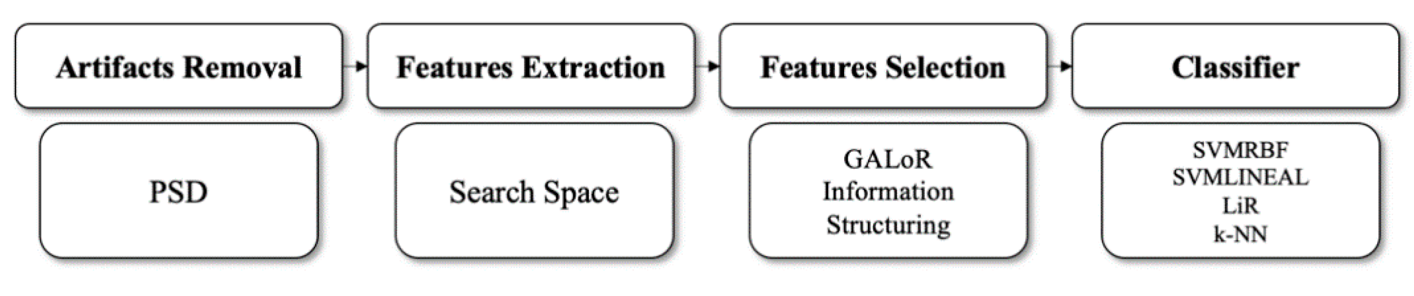
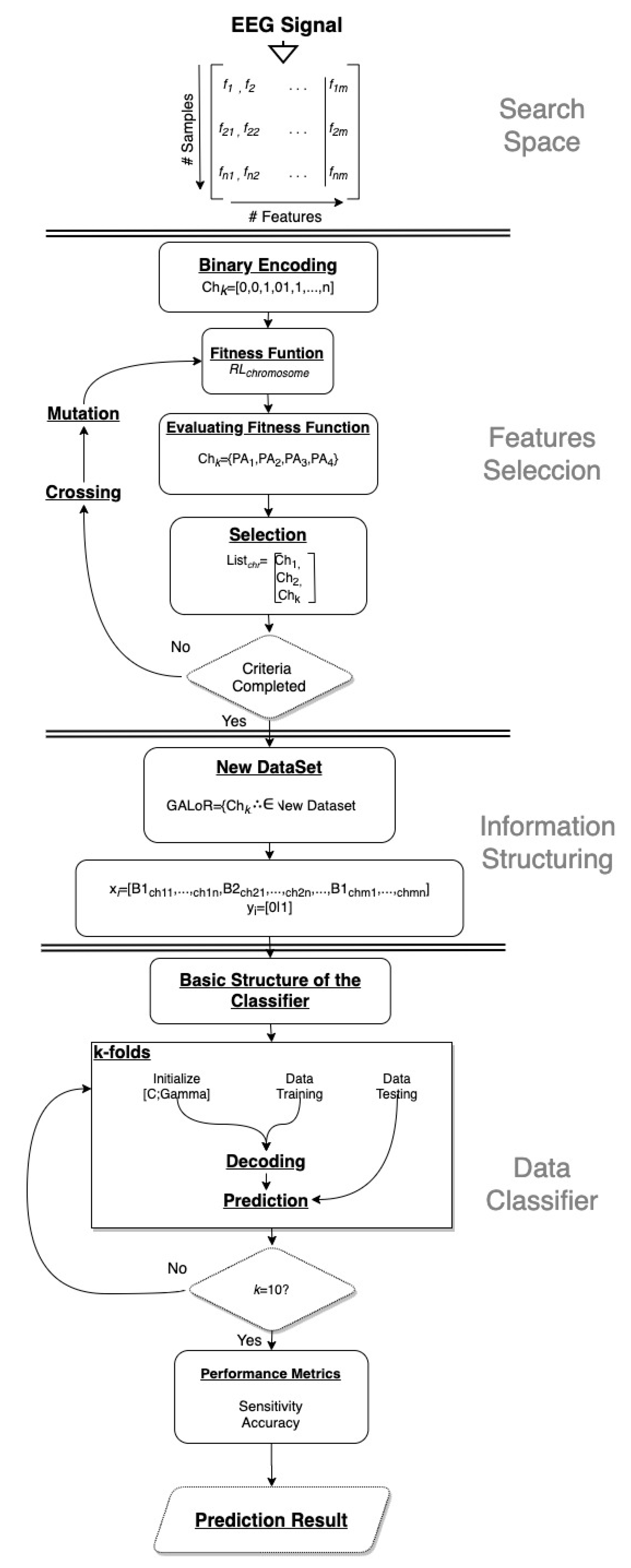
2.2. GALoRIS
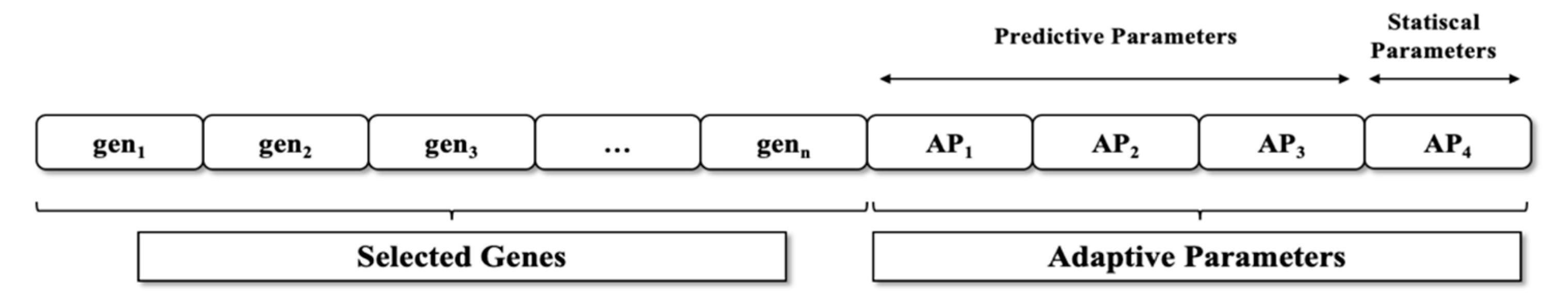
2.3. Population
2.4. Fitness Function
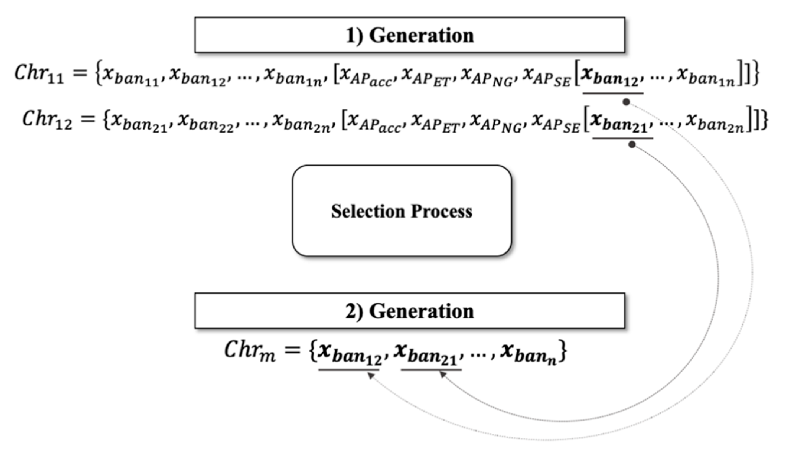
2.5. Selection
2.6. Crossing
2.7. Mutation
2.8. Detection Rules
2.9. Information Structuring
2.10. Classifiers
2.11. Label
3. Experimentation and Materials
3.1. Design of the Experiment
- Baseline: The participant takes a seat and places the Emotiv EPOC sensor on their head [51]. The subject keeps their eyes closed and is acoustically isolated for 10 min, where the sensor is activated to collect information;
- First Task (Task_1): The participant starts driving the vehicle without any distraction. During driving, the EEG signals, ISA, and ER are collected. In the end, NASA-TLX is applied;
- Second task (Task_2): In order to increase the subject’s cognitive workload levels, the stress induction protocol proposed in [7] is applied as a second task. The task consists of the random mentioning of a series of digits that the participant has to repeat, following the order of the set of numbers given. All measurements are collected.
3.2. Subjective Measures
3.3. Measurement of the Vehicle Performance
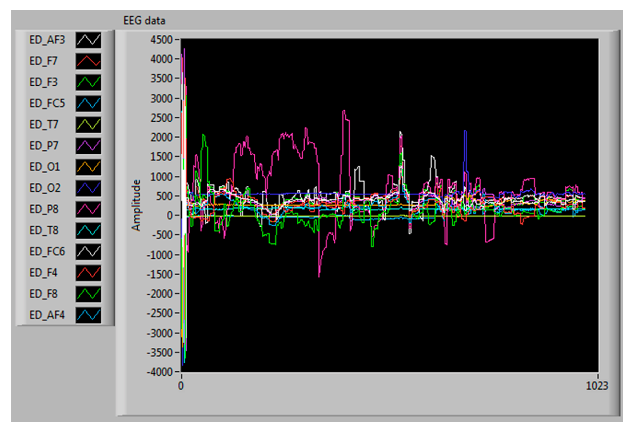
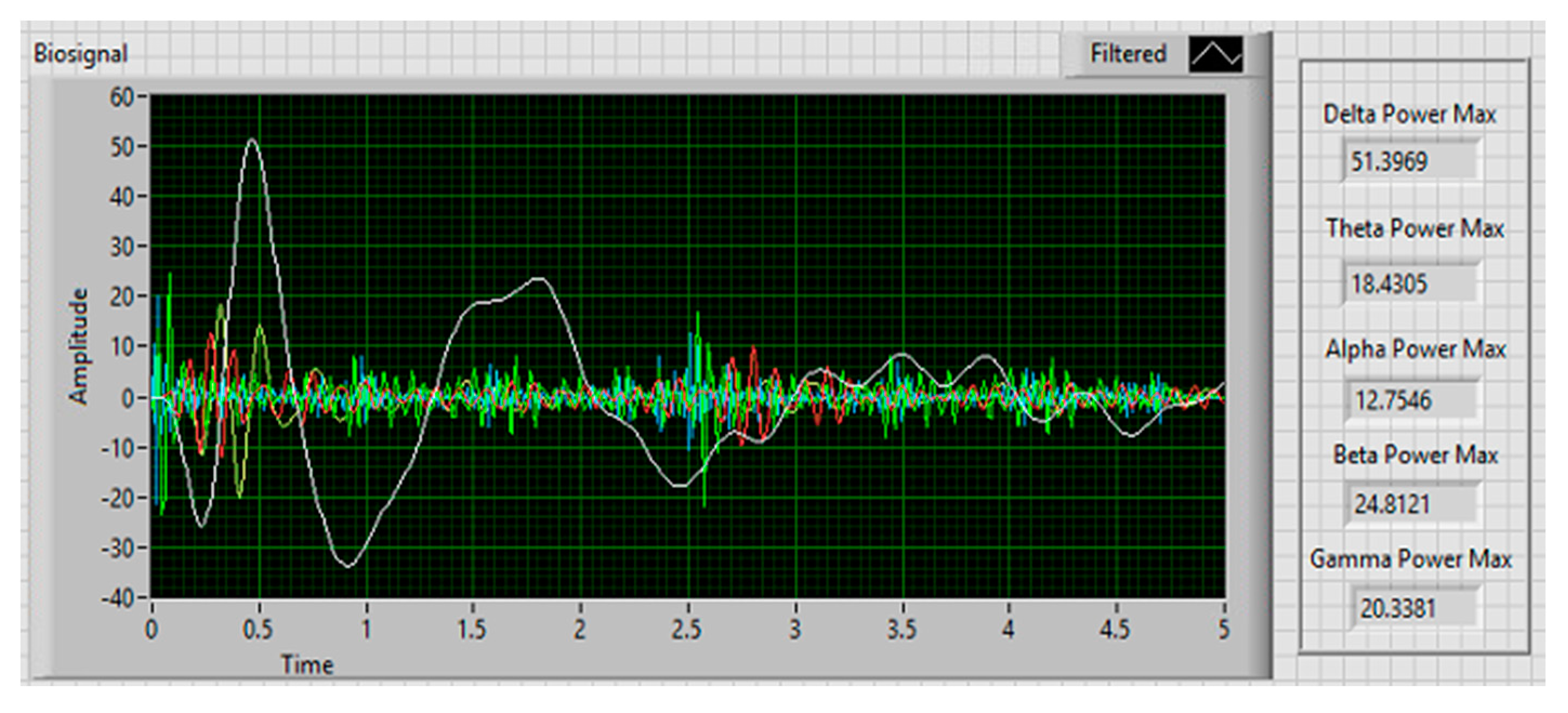
3.4. Collection and Extraction of EEG Signals
3.5. Dataset and Parameters
4. Results
4.1. Subjective and Vehicle Performance Measures
4.2. EEG Signals
4.3. Statistical Test Results
4.4. Labeling Results
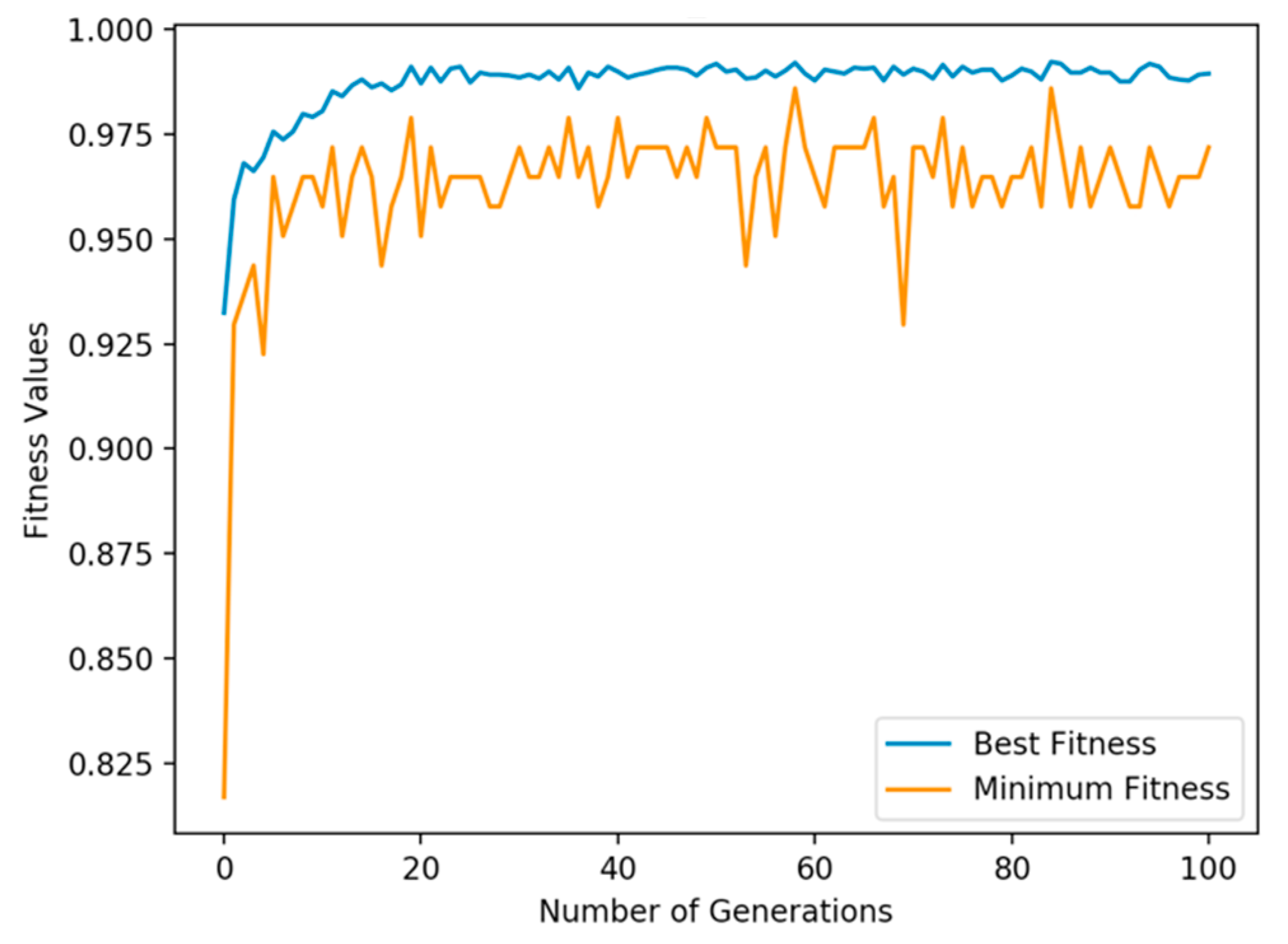
4.5. GALoRIS Results
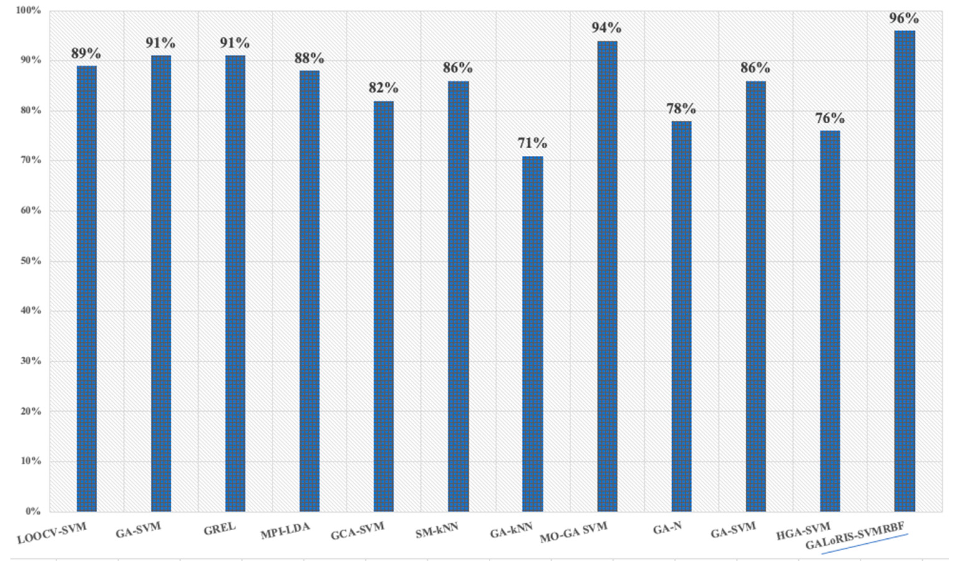
4.6. Classifier Results
5. Conclusions and Discussion
Author Contributions
Funding
Conflicts of Interest
Data Availability
Ethical Statement
References
- Yan, L.; Huang, Z.; Zhang, Y.; Zhang, L.; Zhu, D.; Ran, B. Driving risk status prediction using Bayesian networks and logistic regression. IET Intell. Transp. Syst. 2017, 11, 431–439. [Google Scholar] [CrossRef]
- NASA TLX: Task Load Index NASA TLX. Available online: https://humansystems.arc.nasa.gov/groups/TLX/tlxapp.php (accessed on 3 July 2019).
- Instantaneous Self Assessment of Workload (ISA). Available online: https://ext.eurocontrol.int/ehp/?q=node/1585 (accessed on 3 July 2019).
- Faure, V.; Lobjois, R.; Benguigui, N. The effects of driving environment complexity and dual tasking on drivers’ mental workload and eye blink behavior. Transp. Res. Part F Traffic Psychol. Behav. 2016, 40, 78–90. [Google Scholar] [CrossRef]
- Liu, J.; Gardi, A.; Ramasamy, S.; Lim, Y.; Sabatini, R. Cognitive pilot-aircraft interface for single-pilot operations. Knowl. Based Syst. 2016, 112, 37–53. [Google Scholar] [CrossRef]
- Dussault, C.; Jouanin, J.-C.; Philippe, M.; Guezennec, C.-Y. EEG and ECG changes during simulator operation reflect mental workload and vigilance. Aviat. Space. Environ. Med. 2005, 76, 344–351. [Google Scholar] [PubMed]
- Jacobé de Naurois, C.; Bourdin, C.; Stratulat, A.; Diaz, E.; Vercher, J.L. Detection and prediction of driver drowsiness using artificial neural network models. Accid. Anal. Prev. 2019, 126, 95–104. [Google Scholar] [CrossRef]
- Cao, L.; Li, J.; Xu, Y.; Zhu, H.; Jiang, C. A Hybrid Vigilance Monitoring Study for Mental Fatigue and Its Neural Activities. Cognit. Comput. 2016, 8, 228–236. [Google Scholar] [CrossRef]
- Baig, M.Z.; Aslam, N.; Shum, H.P.H. Filtering techniques for channel selection in motor imagery EEG applications: A survey. Artif. Intell. Rev. 2019. [Google Scholar] [CrossRef] [Green Version]
- Wang, L.; Xue, W.; Li, Y.; Luo, M.; Huang, J.; Cui, W.; Huang, C. Automatic epileptic seizure detection in EEG signals using multi-domain feature extraction and nonlinear analysis. Entropy 2017, 19, 222. [Google Scholar] [CrossRef]
- Nakisa, B.; Rastgoo, M.N.; Tjondronegoro, D.; Chandran, V. Evolutionary computation algorithms for feature selection of EEG-based emotion recognition using mobile sensors. Expert Syst. Appl. 2018, 93, 143–155. [Google Scholar] [CrossRef] [Green Version]
- Bhatti, M.H.; Khan, J.; Khan, M.U.G.; Iqbal, R.; Aloqaily, M.; Jararweh, Y.; Gupta, B. Soft Computing-Based EEG Classification by Optimal Feature Selection and Neural Networks. IEEE Trans. Ind. Inform. 2019, 15, 5747–5754. [Google Scholar] [CrossRef]
- Tao, W.; Li, C.; Song, R.; Cheng, J.; Liu, Y.; Chen, X. EEG-based Emotion Recognition via Channel-wise Attention and Self Attention. IEEE Trans. Affect. Comput. 2020, 1–12. [Google Scholar] [CrossRef]
- Liu, Y.; Ding, Y.; Li, C.; Cheng, J.; Song, R.; Wan, F.; Chen, X. Multi-channel EEG-based emotion recognition via a multi-level features guided capsule network. Comput. Biol. Med. 2020, 123, 103927. [Google Scholar] [CrossRef] [PubMed]
- Wang, Z.M.; Hu, S.Y.; Song, H. Channel Selection Method for EEG Emotion Recognition Using Normalized Mutual Information. IEEE Access 2019, 7, 143303–143311. [Google Scholar] [CrossRef]
- Peterson, V.; Wyser, D.; Lambercy, O.; Spies, R.; Gassert, R. A penalized time-frequency band feature selection and classification procedure for improved motor intention decoding in multichannel EEG. J. Neural Eng. 2019, 16, 16019. [Google Scholar] [CrossRef] [Green Version]
- Tavares, G.; San-Martin, R.; Ianof, J.N.; Anghinah, R.; Fraga, F.J. Improvement in the automatic classification of Alzheimer’s disease using EEG after feature selection. In Proceedings of the 2019 IEEE International Conference on Systems, Man and Cybernetics (SMC), Bari, Italy, 6–9 October 2019; pp. 1264–1269. [Google Scholar] [CrossRef]
- Arsalan, A.; Majid, M.; Butt, A.R.; Anwar, S.M. Classification of Perceived Mental Stress Using A Commercially Available EEG Headband. IEEE J. Biomed. Health Informatics 2019, 23, 2257–2264. [Google Scholar] [CrossRef]
- Marín-Morales, J.; Higuera-Trujillo, J.L.; Greco, A.; Guixeres, J.; Llinares, C.; Scilingo, E.P.; Alcañiz, M.; Valenza, G. Affective computing in virtual reality: Emotion recognition from brain and heartbeat dynamics using wearable sensors. Sci. Rep. 2018, 8, 1–15. [Google Scholar] [CrossRef]
- Batres-Mendoza, P.; Montoro-Sanjose, C.R.; Guerra-Hernandez, E.I.; Almanza-Ojeda, D.L.; Rostro-Gonzalez, H.; Romero-Troncoso, R.J.; Ibarra-Manzano, M.A. Quaternion-based signal analysis for motor imagery classification from electroencephalographic signals. Sensors 2016, 16, 336. [Google Scholar] [CrossRef] [Green Version]
- Sun, H.; Xiang, Y.; Sun, Y.; Zhu, H.; Zeng, J. On-line EEG classification for brain-computer interface based on CSP and SVM. In Proceedings of the 2010 3rd International Congress on Image and Signal Processing, Yantai, China, 16–18 October 2010; Volume 9, pp. 4105–4108. [Google Scholar]
- Bhattacharyya, S.; Khasnobish, A.; Chatterjee, S.; Konar, A.; Tibarewala, D.N. Performance analysis of LDA, QDA and KNN algorithms in left-right limb movement classification from EEG data. In Proceedings of the 2010 International Conference on Systems in Medicine and Biology, Istanbul, Turkey, 10–13 October 2010; pp. 126–131. [Google Scholar]
- Guo, Z.; Pan, Y.; Zhao, G.; Cao, S.; Zhang, J. Detection of Driver Vigilance Level Using EEG Signals and Driving Contexts. IEEE Trans. Reliab. 2018, 67, 370–380. [Google Scholar] [CrossRef]
- Wei, Z.; Zhuang, D.; Wanyan, X.; Liu, C.; Zhuang, H. A model for discrimination and prediction of mental workload of aircraft cockpit display interface. Chinese J. Aeronaut. 2014, 27, 1070–1077. [Google Scholar] [CrossRef] [Green Version]
- Zhang, Y.; Wang, Y.; Zhou, G.; Jin, J.; Wang, B.; Wang, X.; Cichocki, A. Multi-kernel extreme learning machine for EEG classification in brain-computer interfaces. Expert Syst. Appl. 2018, 96, 302–310. [Google Scholar] [CrossRef]
- Chen, L.L.; Zhao, Y.; Ye, P.F.; Zhang, J.; Zou, J.Z. Detecting driving stress in physiological signals based on multimodal feature analysis and kernel classifiers. Expert Syst. Appl. 2017, 85, 279–291. [Google Scholar] [CrossRef]
- Rahmad, C.; Ariyanto, R.; Rizky, D. Brain Signal Classification using Genetic Algorithm for Right-Left Motion Pattern. Int. J. Adv. Comput. Sci. Appl. 2018, 9, 247–251. [Google Scholar] [CrossRef]
- Pal, S.K.; Wang, P.P. Genetic Algorithms for Pattern Recognition; CRC Press: Boca Raton, FL, USA, 2017. [Google Scholar]
- Phan, A.V.; Le Nguyen, M.; Bui, L.T. Feature weighting and SVM parameters optimization based on genetic algorithms for classification problems. Appl. Intell. 2017, 46, 455–469. [Google Scholar] [CrossRef]
- Murugappan, M.; Murugappan, S. Human Emotion Recognition Through Short Time Electroencephalogram (EEG) Signals Using Fast Fourier Transform (FFT). In Proceedings of the IEEE 9th International Colloquium on Signal Processing and its Applications, Kuala Lumpur, Malaysia, 8–10 March 2013; pp. 289–294. [Google Scholar] [CrossRef]
- Yan, S.; Tran, C.C.; Wei, Y.; Habiyaremye, J.L. Driver’s mental workload prediction model based on physiological indices. Int. J. Occup. Saf. Ergon. 2017, 25, 1–9. [Google Scholar] [CrossRef] [PubMed]
- Jenke, R.; Peer, A.; Buss, M. Feature extraction and selection for emotion recognition from EEG. IEEE Trans. Affect. Comput. 2014, 5, 327–339. [Google Scholar] [CrossRef]
- Koelstra, S.; Mühl, C.; Soleymani, M.; Lee, J.S.; Yazdani, A.; Ebrahimi, T.; Pun, T.; Nijholt, A.; Patras, I. DEAP: A database for emotion analysis; Using physiological signals. IEEE Trans. Affect. Comput. 2012, 3, 18–31. [Google Scholar] [CrossRef] [Green Version]
- Nuamah, J.K.; Seong, Y. Neural correspondence to human cognition from analysis to intuition-implications of display design for cognition. Proc. Hum. Factors Ergon. Soc. 2017, 2017, 51–55. [Google Scholar] [CrossRef] [Green Version]
- Di Flumeri, G.; Aricò, P.; Borghini, G.; Sciaraffa, N.; Di Florio, A.; Babiloni, F. The dry revolution: Evaluation of three different eeg dry electrode types in terms of signal spectral features, mental states classification and usability. Sensors 2019, 19, 1365. [Google Scholar] [CrossRef] [Green Version]
- Lin, C.T.; Chuang, C.H.; Huang, C.S.; Tsai, S.F.; Lu, S.W.; Chen, Y.H.; Ko, L.W. Wireless and wearable EEG system for evaluating driver vigilance. IEEE Trans. Biomed. Circuits Syst. 2014, 8, 165–176. [Google Scholar]
- Huo, X.Q.; Zheng, W.L.; Lu, B.L. Driving fatigue detection with fusion of EEG and forehead EOG. In Proceedings of the 2016 International Joint Conference on Neural Networks (IJCNN), Vancouver, BC, Canada, 24–29 July 2016; pp. 897–904. [Google Scholar] [CrossRef]
- Beheshti, I.; Demirel, H.; Matsuda, H. Classification of Alzheimer’s disease and prediction of mild cognitive impairment-to-Alzheimer’s conversion from structural magnetic resource imaging using feature ranking and a genetic algorithm. Comput. Biol. Med. 2017, 83, 109–119. [Google Scholar] [CrossRef]
- Tantithamthavorn, C.; McIntosh, S.; Hassan, A.E.; Matsumoto, K. An Empirical Comparison of Model Validation Techniques for Defect Prediction Models. IEEE Trans. Softw. Eng. 2017, 43, 1–18. [Google Scholar] [CrossRef]
- Al-Shargie, F.; Tang, T.B.; Badruddin, N.; Kiguchi, M. Towards multilevel mental stress assessment using SVM with ECOC: An EEG approach. Med. Biol. Eng. Comput. 2018, 56, 125–136. [Google Scholar] [CrossRef]
- B-Alert Cognitive-Affective Metrics. Available online: https://imotions.com/blog/eeg/ (accessed on 20 January 2020).
- Eldenfria, A.; Al-Samarraie, H. Towards an Online Continuous Adaptation Mechanism (OCAM) for Enhanced Engagement: An EEG Study. Int. J. Hum. Comput. Interact. 2019, 35, 1960–1974. [Google Scholar] [CrossRef]
- Kamzanova, A.; Kustubayeva, A.; Matthews, G. Diagnostic monitoring of vigilance decrement using EEG workload indices. In Proceedings of the Human Factors and Ergonomics Society Annual Meeting; Sage Publications Sage CA: Los Angeles, CA, USA, 2012; Volume 56, pp. 203–207. [Google Scholar]
- Ramirez, R.; Palencia-Lefler, M.; Giraldo, S.; Vamvakousis, Z. Musical neurofeedback for treating depression in elderly people. Front. Neurosci. 2015, 9, 354. [Google Scholar] [CrossRef] [Green Version]
- Fiscon, G.; Weitschek, E.; Cialini, A.; Felici, G.; Bertolazzi, P.; De Salvo, S.; Bramanti, A.; Bramanti, P.; De Cola, M.C. Combining EEG signal processing with supervised methods for Alzheimer’s patients classification. BMC Med. Inform. Decis. Mak. 2018, 18, 35. [Google Scholar] [CrossRef]
- Nuamah, J.K.; Seong, Y. Support vector machine (SVM) classification of cognitive tasks based on electroencephalography (EEG) engagement index. Brain-Comput. Interfaces 2018, 5, 1–12. [Google Scholar] [CrossRef]
- Petrantonakis, P.C.; Leontios, J. EEG-based emotion recognition using advanced signal processing techniques. Emot. Recognit. A Pattern Anal. Approach 2014, 269–293. [Google Scholar] [CrossRef]
- Milind Gaikwad Effect of Meditation on Cognitive Workload. In EEG-Based Emotion Analysis and Recognition; SGGS IET, Nanded: Maharashtra, India, 2019; pp. 88–107.
- Krause, M. LCT FOR SILAB. Available online: https://www.lfe.mw.tum.de/en/downloads/open-source-tools/lct-for-silab/ (accessed on 30 September 2019).
- Mattes, S.; Hallén, A. Surrogate distraction measurement techniques: The lane change test. Driv. Distraction Theory Eff. Mitig. 2009, 107–121. [Google Scholar] [CrossRef]
- Zhong, N.; Bradshaw, J.M.; Liu, J.; Taylor, J.G. Detecting Emotion from EEG Signals Using the Emotive Epoc Device. IEEE Intell. Syst. 2011, 26, 16–21. [Google Scholar] [CrossRef]
- Tattersall, A.J.; Foord, P.S. An experimental evaluation of instantaneous self-assessment as a measure of workload. Ergonomics 1996, 39, 740–748. [Google Scholar] [CrossRef]
- Yu, K.; Prasad, I.; Mir, H.; Thakor, N.; Al-Nashash, H. Cognitive workload modulation through degraded visual stimuli: A single-trial EEG study. J. Neural Eng. 2015, 12. [Google Scholar] [CrossRef] [PubMed] [Green Version]
- Kim, H.S.; Hwang, Y.; Yoon, D.; Choi, W.; Park, C.H. Driver workload characteristics analysis using EEG data from an urban road. IEEE Trans. Intell. Transp. Syst. 2014, 15, 1844–1849. [Google Scholar] [CrossRef]
- Kim, M.M.-K.; Kim, M.M.-K.; Oh, E.; Kim, S.-P. A Review on the Computational Methods for Emotional State Estimation from the Human EEG. Comput. Math. Methods Med. 2013, 2013, 573734. [Google Scholar] [CrossRef] [PubMed] [Green Version]
- Engström, J.; Markkula, G. Effects of visual and cognitive distraction on lane change test performance. In Proceedings of the Fourth International Driving Symposium on Human Factors in Driver Assessment, Training and Vehicle Design, Stevenson, WA, USA, 9–12 July 2007; Volume 4. [Google Scholar]
- Young, K.L.; Lenné, M.G.; Williamson, A.R. Sensitivity of the lane change test as a measure of in-vehicle system demand. Appl. Ergon. 2011, 42, 611–618. [Google Scholar] [CrossRef]
- Daud, S.S.; Sudirman, R. Butterworth Bandpass and Stationary Wavelet Transform Filter Comparison for Electroencephalography Signal. Proc. Int. Conf. Intell. Syst. Model. Simul. ISMS 2015, 2015, 123–126. [Google Scholar] [CrossRef]
- Becerra-Sánchez, E.P.; Reyes-Muñoz, A.; Guerrero-Ibáñez, J.A. Wearable Sensors for Evaluating Driver Drowsiness and High Stress. IEEE Lat. Am. Trans. 2019, 17, 418–425. [Google Scholar] [CrossRef]
- Kamzanova, A.T.; Kustubayeva, A.M.; Matthews, G. Use of EEG workload indices for diagnostic monitoring of vigilance decrement. Hum. Factors 2014, 56, 1136–1149. [Google Scholar] [CrossRef]
- Nandish, M.; Michahial, S.; P, H.K.; Ahmed, F. Feature Extraction and Classification of EEG Signal Using Neural Network Based Techniques. Int. J. Eng. Innov. Technol. 2012, 2, 1–5. [Google Scholar] [CrossRef]
- Yuvaraj, R.; Murugappan, M.; Ibrahim, N.M.; Omar, M.I.; Sundaraj, K.; Mohamad, K.; Palaniappan, R.; Mesquita, E.; Satiyan, M. On the analysis of EEG power, frequency and asymmetry in Parkinson’s disease during emotion processing. Behav. Brain Funct. 2014, 10, 12. [Google Scholar] [CrossRef] [Green Version]
- Parvinnia, E.; Sabeti, M.; Jahromi, M.Z.; Boostani, R. Classification of EEG Signals using adaptive weighted distance nearest neighbor algorithm. J. King Saud Univ. Inf. Sci. 2014, 26, 1–6. [Google Scholar] [CrossRef] [Green Version]
- Riaz, F.; Hassan, A.; Rehman, S.; Niazi, I.K.; Dremstrup, K. EMD-based temporal and spectral features for the classification of EEG signals using supervised learning. IEEE Trans. Neural Syst. Rehabil. Eng. 2015, 24, 28–35. [Google Scholar] [CrossRef]
- Zammouri, A.; Chraa-Mesbahi, S.; Ait Moussa, A.; Zerouali, S.; Sahnoun, M.; Tairi, H.; Mahraz, A.M. Brain waves-based index for workload estimation and mental effort engagement recognition. J. Phys. Conf. Ser. 2017, 904. [Google Scholar] [CrossRef] [Green Version]
- Puma, S.; Matton, N.; Paubel, P.-V.V.; Raufaste, É.; El-Yagoubi, R. Using theta and alpha band power to assess cognitive workload in multitasking environments. Int. J. Psychophysiol. 2018, 123, 111–120. [Google Scholar] [CrossRef]
- Nuamah, J.K.; Seong, Y.; Yi, S. Electroencephalography (EEG) classification of cognitive tasks based on task engagement index. In Proceedings of the 2017 IEEE Conference on Cognitive and Computational Aspects of Situation Management (CogSIMA), Savannah, GA, USA, 27–31 March 2017; pp. 1–6. [Google Scholar]
- Jap, B.T.; Lal, S.; Fischer, P. Comparing combinations of EEG activity in train drivers during monotonous driving. Expert Syst. Appl. 2011, 38, 996–1003. [Google Scholar] [CrossRef]
- Lin, Q.; Huang, J.B.; Zhong, J.; Lin, S.; Xue, Y. Feature selection and recognition of electroencephalogram signals: An extreme learning machine and genetic algorithm-based approach. Proc. Int. Conf. Mach. Learn. Cybern. 2015, 2, 499–504. [Google Scholar] [CrossRef]
- Tao, P.; Sun, Z.; Sun, Z. An Improved Intrusion Detection Algorithm Based on GA and SVM. IEEE Access 2018, 6, 13624–13631. [Google Scholar] [CrossRef]
- Johnson, P.; Vandewater, L.; Wilson, W.; Maruff, P.; Savage, G.; Graham, P.; Macaulay, L.S.; Ellis, K.A.; Szoeke, C.; Martins, R.N.; et al. Genetic algorithm with logistic regression for prediction of progression to Alzheimer’s disease. BMC Bioinform. 2014, 15, S11. [Google Scholar] [CrossRef] [Green Version]
- Matthews, G.; Reinerman-Jones, L.E.; Barber, D.J.; Abich, J. The psychometrics of mental workload: Multiple measures are sensitive but divergent. Hum. Factors 2015, 57, 125–143. [Google Scholar] [CrossRef]
- Amo, C.; de Santiago, L.; Barea, R.; López-Dorado, A.; Boquete, L. Analysis of gamma-band activity from human EEG using empirical mode decomposition. Sensors 2017, 17, 989. [Google Scholar] [CrossRef] [Green Version]
- Mahmoudi, M.; Shamsi, M. Multi-class EEG classification of motor imagery signal by finding optimal time segments and features using SNR-based mutual information. Australas. Phys. Eng. Sci. Med. 2018, 41, 957–972. [Google Scholar] [CrossRef]
- Tian, Y.; Xu, W.; Yang, L. Cortical Classification with Rhythm Entropy for Error Processing in Cocktail Party Environment Based on Scalp EEG Recording. Sci. Rep. 2018, 8, 1–13. [Google Scholar] [CrossRef] [PubMed] [Green Version]
- Zheng, W.L.; Lu, B.L. A multimodal approach to estimating vigilance using EEG and forehead EOG. J. Neural Eng. 2017, 14. [Google Scholar] [CrossRef] [PubMed]
- Zhao, H.; Guo, X.; Wang, M.; Li, T.; Pang, C.; Georgakopoulos, D. Analyze EEG signals with extreme learning machine based on PMIS feature selection. Int. J. Mach. Learn. Cybern. 2018, 9, 243–249. [Google Scholar] [CrossRef]
- Li, X.; Chen, X.; Yan, Y.; Wei, W.; Wang, Z.J. Classification of EEG signals using a multiple kernel learning support vector machine. Sensors 2014, 14, 12784–12802. [Google Scholar] [CrossRef] [PubMed] [Green Version]
- Bajaj, V.; Taran, S.; Sengur, A. Emotion classification using flexible analytic wavelet transform for electroencephalogram signals. Health Inf. Sci. Syst. 2018, 6, 1–7. [Google Scholar] [CrossRef]
- Shon, D.; Im, K.; Park, J.H.; Lim, D.S.; Jang, B.; Kim, J.M. Emotional stress state detection using genetic algorithm-based feature selection on EEG signals. Int. J. Environ. Res. Public Health 2018, 15. [Google Scholar] [CrossRef] [Green Version]
- Valenzuela, O.; Jiang, X.; Carrillo, A.; Rojas, I. Multi-Objective Genetic Algorithms to Find Most Relevant Volumes of the Brain Related to Alzheimer’s Disease and Mild Cognitive Impairment. Int. J. Neural Syst. 2018, 28. [Google Scholar] [CrossRef]
- Malan, N.S.; Sharma, S. Feature selection using regularized neighbourhood component analysis to enhance the classification performance of motor imagery signals. Comput. Biol. Med. 2019, 107, 118–126. [Google Scholar] [CrossRef]
- Cai, H.; Qu, Z.; Li, Z.; Zhang, Y.; Hu, X.; Hu, B. Feature-level fusion approaches based on multimodal EEG data for depression recognition. Inf. Fusion 2020, 59, 127–138. [Google Scholar] [CrossRef]
- Leon, M.; Ballesteros, J.; Tidare, J.; Xiong, N.; Astrand, E. Feature Selection of EEG Oscillatory Activity Related to Motor Imagery Using a Hierarchical Genetic Algorithm. In Proceedings of the 2019 IEEE Congress on Evolutionary Computation (CEC) Wellington, New Zealan, 10–13 June 2019; pp. 87–94. [Google Scholar] [CrossRef]
- Ramezan, C.A.; Warner, T.A.; Maxwell, A.E. Evaluation of sampling and cross-validation tuning strategies for regional-scale machine learning classification. Remote Sens. 2019, 11. [Google Scholar] [CrossRef] [Green Version]


| References | States | Metrics |
|---|---|---|
| [40] | Lateral Index at Stress | |
| [41] | Cognitive-Affective (Frontal Asymmetry) | |
| [42] | Engagement | |
| [43] | Alert/Stress | |
| [44] | Valence | |
| [44] | Arousal | |
| [45] | Alzheimer | |
| [46] | Event-related desynchronization | |
| [47] | Neuronal activity | |
| [48] | Load Index | |
| [48] | Equanimity |
| Dataset | Features | No. of Features |
|---|---|---|
| Subset_1 | Delta_AF4,Delta_T8,Delta_AF3,Delta_F3, Delta_F7, Delta_F8, Delta_FC5, Delta_O2, Delta_P8, Alpha_AF4, Alpha_F3, Alpha_F7, Alpha_F8, Alpha_FC5, Alpha_O2, Alpha_P8, Alpha_T8, Beta_AF3, Beta_AF4, Beta_F3, Beta_F7, Beta_F8, Beta_FC5, Beta_O2, Beta_P8, Beta_T8, Gamma_AF4, Gamma_F3, Gamma_F7, Gamma_F8, Gamma_FC5, Gamma_O2, Gamma_P8, Gamma_T8 | 36 |
| Subset_2 | Alpha_AF4, Alpha_F3, Alpha_F7, Alpha_F8, Alpha_FC5, Alpha_O2, Alpha_P8, Alpha_T8 | 9 |
| Subset_3 | Beta_AF4, Beta_F3, Beta_F7, Beta_F8, Beta_FC5, Beta_O2, Beta_P8, Beta_T8, Gamma_AF4, Gamma_F3, Gamma_F7, Gamma_F8, Gamma_FC5, Gamma_O2, Gamma_P8, Gamma_T8 | 18 |
| Subset_4 | Alpha_AF4, Alpha_F3, Alpha_F7, Alpha_F8, Alpha_FC5, Alpha_O2, Alpha_P8, Alpha_T8, Beta_AF3, Beta_AF4, Beta_F3, Beta_F7, Beta_F8, Beta_FC5, Beta_O2, Beta_P8, Beta_T8, | 18 |
| Subset_5 | Alpha_AF4, Alpha_F3, Alpha_F7, Alpha_F8, Alpha_FC5, Alpha_O2, Alpha_P8, Alpha_T8, Beta_AF3, Beta_AF4, Beta_F3, Beta_F7, Beta_F8, Beta_FC5, Beta_O2, Beta_P8, Beta_T8, Gamma_AF4, Gamma_F3, Gamma_F7, Gamma_F8, Gamma_FC5, Gamma_O2, Gamma_P8, Gamma_T8 | 27 |
| Subset_6 | Delta_AF4, Delta_T8, Delta_AF3, Delta_F3, Delta_F7, Delta_F8, Delta_FC5, Delta_O2, Delta_P8, Alpha_AF4, Alpha_F3, Alpha_F7, Alpha_F8, Alpha_FC5, Alpha_O2, Alpha_P8, Alpha_T8, Beta_AF3, Beta_AF4, Beta_F3, Beta_F7, Beta_F8, Beta_FC5, Beta_O2, Beta_P8, Beta_T8 | 27 |
| Subset_7 | Delta_AF4, Delta_T8, Delta_AF3, Delta_F3, Delta_F7, Delta_F8, Delta_FC5, Delta_O2, Delta_P8, Alpha_AF4, Alpha_F3, Alpha_F7, Alpha_F8, Alpha_FC5, Alpha_O2, Alpha_P8, Alpha_T8, Gamma_AF4, Gamma_F3, Gamma_F7, Gamma_F8, Gamma_FC5, Gamma_O2, Gamma_P8, Gamma_T8 | 27 |
| ISA | NASA-TLX | ER | ||||
|---|---|---|---|---|---|---|
| Subjects | Task_1 | Task_2 | Task_1 | Task_2 | Task_1 | Task_2 |
| Subject_1 | 16.66 | 34.44 | 4.33 | 65.67 | 3 | 12 |
| Subject_3 | 31.10 | 57.77 | 12.67 | 56.67 | 4 | 7 |
| Subject_4 | 25.55 | 51.10 | 20.33 | 70.67 | 3 | 8 |
| Subject_5 | 21.10 | 43.33 | 64.33 | 68.67 | 2 | 4 |
| Total | 23.10 | 43.32 | 28.33 | 61.80 | 19 | 34 |
| Bands | Task | Mean | Std. Deviation |
|---|---|---|---|
| Delta | Task_1 | 10.9193 | 1.20741 |
| Task_2 | 9.8171 | 0.5733 | |
| Theta | Task_1 | 10.2063 | 0.4682 |
| Task_2 | 9.9971 | 0.11242 | |
| Alpha | Task_1 | 10.4613 | 0.48171 |
| Task_2 | 10.6696 | 0.46037 | |
| Beta | Task_1 | 22.4447 | 0.89813 |
| Task_2 | 23.2951 | 0.3818 | |
| Gamma | Task_1 | 15.5624 | 0.19241 |
| Task_2 | 15.8033 | 0.16196 |
| Task_1 | Task_2 | p-Value | |
|---|---|---|---|
| M ± SD | M ± SD | ||
| NASA-TLX | 25.41 ± 715.7 | 65.42 ± 38.25 | p ≤ 0.048 |
| ISA | 23.60 ± 38.18 | 46.66 ± 101.24 | p ≤ 0.001 |
| ER | 3 ± 0.66 | 8.25 ± 8.25 | p ≤ 0.028 |
| DELTA | 0.106 ± 0.084 | 0.028 ± 0.040 | p ≤ 0.038 |
| THETA | 0.056 ± 0.032 | 0.041 ± 0.007 | p ≤ 0.383 |
| ALPHA | 0.074 ± 0.033 | 0.088 ± 0.032 | p ≤ 0.05 |
| BETA | 0.917 ± 0.063 | 0.977 ± 0.026 | p ≤ 0.036 |
| GAMMA | 0.432 ± 0.013 | 0.449 ± 0.011 | p ≤ 0.005 |
| Subjective | Performance | Physiological Measures | ||||||
|---|---|---|---|---|---|---|---|---|
| ISA | NASA | RT | Alpha | Beta | Delta | Gamma | Theta | |
| ISA | --- | |||||||
| NASA | 0.598 | --- | ||||||
| RT | 0.612 | 0.538 | --- | |||||
| Alpha | 0.301 | −0.168 | 0.680 | --- | ||||
| Beta | 0.488 | −0.113 | 0.642 | 0.873 | --- | |||
| Delta | −0.519 | −0.097 | −0.745 | −0.830 | −0.894 | --- | ||
| Gamma | 0.610 | 0.062 | 0.815 | 0.851 | 0.856 | −0.805 | --- | |
| Theta | −0.121 | 0.206 | −0.247 | −0.592 | −0.727 | 0.768 | −0.329 | --- |
| Subset | Chromosomes | Features Selection | # Gens | Acc | ER | Time (s) |
|---|---|---|---|---|---|---|
| Subset 1 | [0,1,1,1,0,0,0,1,0,1,1,1,1,0,0,0,1,1,0,0,0,1,0,0,0,1,0,0,0,0,1,0,0,0,0,0] | ‘Delta_AF4′, ‘Delta_F3′, ‘Delta_F7′, ‘Delta_P8′, ‘Alpha_AF3′, ‘Alpha_AF4′, ‘Alpha_F3′, ‘Alpha_F7′, ‘Alpha_P8′, ‘Alpha_T8′, ‘Beta_F7′, ‘Beta_P8′, ‘Gamma_F7′ | 13 | 97.7% | 2.26% | 580.84 |
| Subset 2 | [0,0,1,0,1,0,1,0,0] | ‘Alpha_F3′, ‘Alpha_F8′, ‘Alpha_O2′ | 3 | 77.34% | 22.6% | 201.67 |
| Subset 3 | [1,1,1,0,1,1,0,1,1,0,1,0,0,1,1,0,0,1] | ‘Beta_AF3′, ‘Beta_AF4′, ‘Beta_F3′, ‘Beta_F8′, ‘Beta_FC5′, ‘Beta_P8′, ‘Beta_T8′, ‘Gamma_AF4′, ‘Gamma_F8′, ‘Gamma_FC5′, ‘Gamma_T8′ | 11 | 88.7% | 11.2% | 394.05 |
| Subset 4 | [1,1,0,1,1,1,1,1,1,1,1,1,1,0,1,1,1,1] | ‘Alpha_AF3′, ‘Alpha_AF4′, ‘Alpha_F7′, ‘Alpha_F8′, ‘Alpha_FC5′, ‘Alpha_O2′, ‘Alpha_P8′, ‘Alpha_T8′, ‘Beta_AF3′, ‘Beta_AF4′, ‘Beta_F3′, ‘Beta_F7′, ‘Beta_FC5′, ‘Beta_O2′, ‘Beta_P8′, ‘Beta_T8′ | 16 | 94.4% | 5.55% | 455.52 |
| Subset 5 | [0,1,1,1,1,1,1,1,1,0,0,0,1,0,1,1,0,1,1,0,1,0,1,0,1,0,1] | ‘Alpha_AF4′, ‘Alpha_F3′, ‘Alpha_F7′, ‘Alpha_F8′, ‘Alpha_FC5′, ‘Alpha_O2′, ‘Alpha_P8′, ‘Alpha_T8′, ‘Beta_F7′, ‘Beta_FC5′, ‘Beta_O2′, ‘Beta_T8′, ‘Gamma_AF3′, ‘Gamma_F3′, ‘Gamma_F8′, ‘Gamma_O2′, ‘Gamma_T8′ | 17 | 95.4% | 4.51% | 637.29 |
| Subset 61 | [1,0,1,1,0,0,1,1,1,0,1,1,1,1,1,0,0,0,1,1,1,1,0,1,1,0,1] | ‘Delta_AF3′, ‘Delta_F3′, ‘Delta_F7′, ‘Delta_O2′, ‘Delta_P8′, ‘Delta_T8′, ‘Alpha_AF4′, ‘Alpha_F3′, ‘Alpha_F7′, ‘Alpha_F8′, ‘Alpha_FC5′, ‘Beta_AF3′, ‘Beta_AF4′, ‘Beta_F3′, ‘Beta_F7′, ‘Beta_FC5′, ‘Beta_O2′, ‘Beta_T8′ | 18 | 96.5% | 3.42% | 618.34 |
| Subset 62 | [1,0,1,1,1,0,1,1,1,0,0,0,0,0,0,1,0,1,0,1,1,0,0,1,0,0,1] | ‘Delta_AF3′, ‘Delta_F3′, ‘Delta_F7′, ‘Delta_F8′, ‘Delta_O2′, ‘Delta_P8′, ‘Delta_T8′, ‘Alpha_O2′, ‘Alpha_T8′, ‘Beta_AF4′, ‘Beta_F3′, ‘Beta_FC5′, ‘Beta_T8′ | 13 | 96.5% | 3.42% | 618.34 |
| Subset 63 | [1,0,0,1,1,0,1,1,0,0,0,0,0,0,1,0,0,0,1,1,0,0,0,1,1,0,0] | ‘Delta_AF3′, ‘Delta_F7′, ‘Delta_F8′, ‘Delta_O2′, ‘Delta_P8′, ‘Alpha_FC5′, ‘Beta_AF3′, ‘Beta_AF4′, ‘Beta_FC5′, ‘Beta_O2′ | 10 | 96.5% | 3.42% | 618.34 |
| Subset 64 | [0,0,0,0,0,0,0,0,1,1,0,0,1,0,0,0,1,1,1,1,0,0,0,0,1,0,0,1] | ‘Delta_T8′, ‘Alpha_AF3′, ‘Alpha_F7′, ‘Alpha_P8′, ‘Alpha_T8′, ‘Beta_AF3′, ‘Beta_AF4′, ‘Beta_O2′ | 8 | 96.5% | 3.42% | 618.34 |
| Subset 7 | [1,1,0,1,1,0,0,0,1,1,1,1,0,1,0,1,1,0,1,1,1,1,1,1,1,0,1] | ‘Delta_AF3′, ‘Delta_AF4′, ‘Delta_F7′, ‘Delta_F8′, ‘Delta_T8′, ‘Alpha_AF3′, ‘Alpha_AF4′, ‘Alpha_F3′, ‘Alpha_F8′, ‘Alpha_O2′, ‘Alpha_P8′, ‘Gamma_AF3′, ‘Gamma_AF4′, ‘Gamma_F3′, ‘Gamma_F7′, ‘Gamma_F8′, ‘Gamma_FC5′, ‘Gamma_O2′, ‘Gamma_T8′ | 19 | 90.25% | 9.75% | 425.94 |
| Subset | SVMRBF | k-NN | SVMLINEAL | LiR | ||||||||
|---|---|---|---|---|---|---|---|---|---|---|---|---|
| Train | Test | Sens | Train | Test | Sens | Train | Test | Sens | Train | Test | Sens | |
| Subset 1 | 96.77 | 96.71 | 96.64 | 97.67 | 97.50 | 97.50 | 89.38 | 89.29 | 89.36 | 89.57 | 89.43 | 89.46 |
| Subset 2 | 85.50 | 84.36 | 84.34 | 82.59 | 81.66 | 81.89 | 66.03 | 65.97 | 65.92 | 65.02 | 64.96 | 64.94 |
| Subset 3 | 97.61 | 97.02 | 97.00 | 94.91 | 94.26 | 94.38 | 85.60 | 85.57 | 85.53 | 85.02 | 84.87 | 84.92 |
| Subset 4 | 98.27 | 98.16 | 98.08 | 98.70 | 98.50 | 98.50 | 91.02 | 90.73 | 90.68 | 90.25 | 90.09 | 90.06 |
| Subset 5 | 97.70 | 97.27 | 97.28 | 97.61 | 97.46 | 97.42 | 89.66 | 89.50 | 89.40 | 89.06 | 88.91 | 88.89 |
| Subset 61 | 98.38 | 98.24 | 98.28 | 98.76 | 98.64 | 98.60 | 91.39 | 91.27 | 91.18 | 90.79 | 90.59 | 90.78 |
| Subset 62 | 96.75 | 96.54 | 96.57 | 98.40 | 98.17 | 98.20 | 86.90 | 86.86 | 86.80 | 86.52 | 86.47 | 86.38 |
| Subset 63 | 98.54 | 98.27 | 98.27 | 97.28 | 96.90 | 96.98 | 84.71 | 84.64 | 84.49 | 84.58 | 84.45 | 84.43 |
| Subset 64 | 97.97 | 97.72 | 97.67 | 95.38 | 95.03 | 94.84 | 79.97 | 79.96 | 79.90 | 79.59 | 79.50 | 79.51 |
| Subset 7 | 97.55 | 97.17 | 97.14 | 96.73 | 96.50 | 96.35 | 85.08 | 84.94 | 84.78 | 92.95 | 92.82 | 92.80 |
| Total | 96.50 | 96.14 | 96.64 | 95.80 | 95.46 | 95.47 | 84.97 | 84.87 | 84.80 | 85.33 | 85.21 | 85.21 |
| Subset | GALoRIS | MI | PCA | |||||||||
|---|---|---|---|---|---|---|---|---|---|---|---|---|
| SVM RBF | k-NN | SVM | LiR | SVM RBF | k-NN | SVM | LiR | SVM RBF | k-NN | SVM | LiR | |
| Subset 1 | 96.77 | 97.50 | 89.29 | 89.43 | 87.78 | 86.87 | 76.37 | 77.40 | 80.48 | 80.08 | 69.03 | 68.78 |
| Subset 2 | 84.36 | 81.66 | 65.97 | 64.96 | 98.78 | 98.17 | 98.32 | 97.65 | 98.66 | 99.33 | 98.62 | 98.72 |
| Subset 3 | 97.02 | 94.26 | 85.57 | 84.87 | 88.00 | 86.87 | 76.37 | 77.40 | 86.05 | 85.38 | 83.46 | 83.43 |
| Subset 4 | 98.16 | 98.50 | 90.73 | 90.09 | 84.65 | 81.21 | 78.47 | 76.85 | 79.38 | 78.19 | 60.44 | 61.26 |
| Subset 5 | 97.70 | 97.46 | 89.50 | 88.91 | 87.78 | 86.87 | 76.37 | 77.40 | 76.33 | 75.06 | 62.39 | 62.08 |
| Subset 6 | 97.91 | 97.18 | 85.68 | 85.25 | 87.08 | 85.26 | 78.68 | 77.43 | 83.16 | 82.42 | 68.17 | 67.75 |
| Subset 7 | 97.17 | 96.50 | 84.94 | 92.82 | 85.53 | 82.06 | 76.40 | 76.12 | 79.59 | 79.26 | 65.89 | 65.46 |
| Total | 96.14 | 95.46 | 84.87 | 85.21 | 88.51 | 86.76 | 80.14 | 80.04 | 83.38 | 82.82 | 72.57 | 72.50 |
Publisher’s Note: MDPI stays neutral with regard to jurisdictional claims in published maps and institutional affiliations. |
© 2020 by the authors. Licensee MDPI, Basel, Switzerland. This article is an open access article distributed under the terms and conditions of the Creative Commons Attribution (CC BY) license (http://creativecommons.org/licenses/by/4.0/).
Share and Cite
Becerra-Sánchez, P.; Reyes-Munoz, A.; Guerrero-Ibañez, A. Feature Selection Model based on EEG Signals for Assessing the Cognitive Workload in Drivers. Sensors 2020, 20, 5881. https://doi.org/10.3390/s20205881
Becerra-Sánchez P, Reyes-Munoz A, Guerrero-Ibañez A. Feature Selection Model based on EEG Signals for Assessing the Cognitive Workload in Drivers. Sensors. 2020; 20(20):5881. https://doi.org/10.3390/s20205881
Chicago/Turabian StyleBecerra-Sánchez, Patricia, Angelica Reyes-Munoz, and Antonio Guerrero-Ibañez. 2020. "Feature Selection Model based on EEG Signals for Assessing the Cognitive Workload in Drivers" Sensors 20, no. 20: 5881. https://doi.org/10.3390/s20205881