Polarization Differential Visible Light Communication: Theory and Experimental Evaluation †


Abstract
:1. Introduction
2. System Model
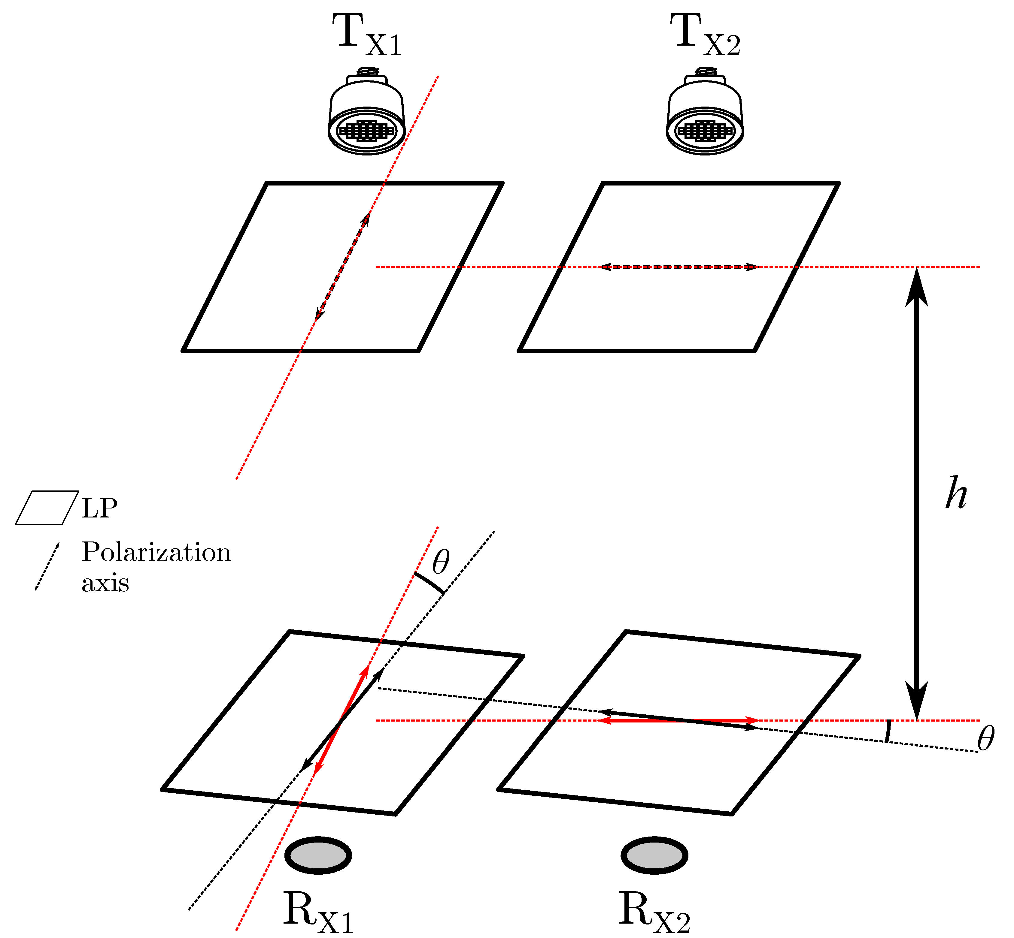
2.1. Polarization
2.2. Modulation and Demodulation
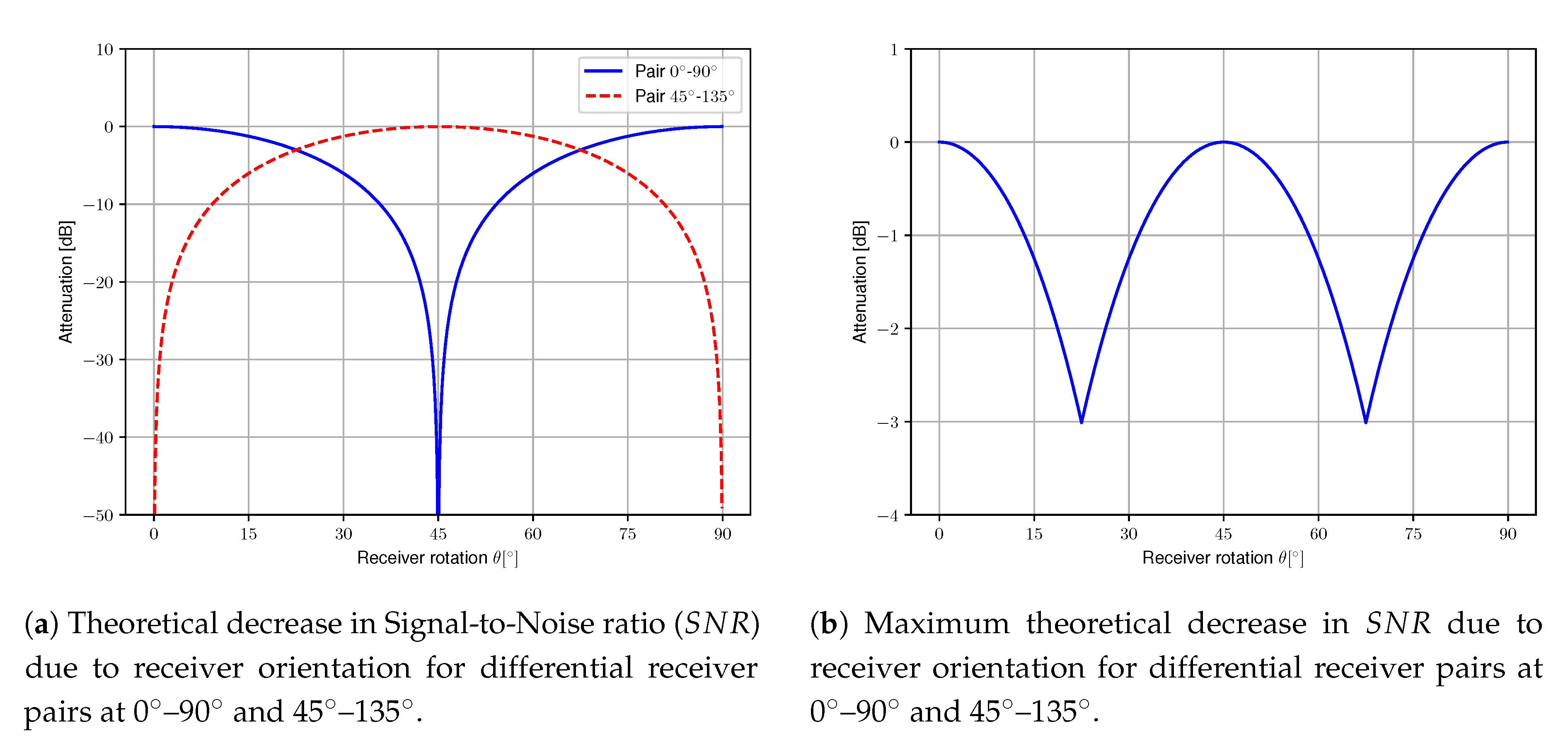
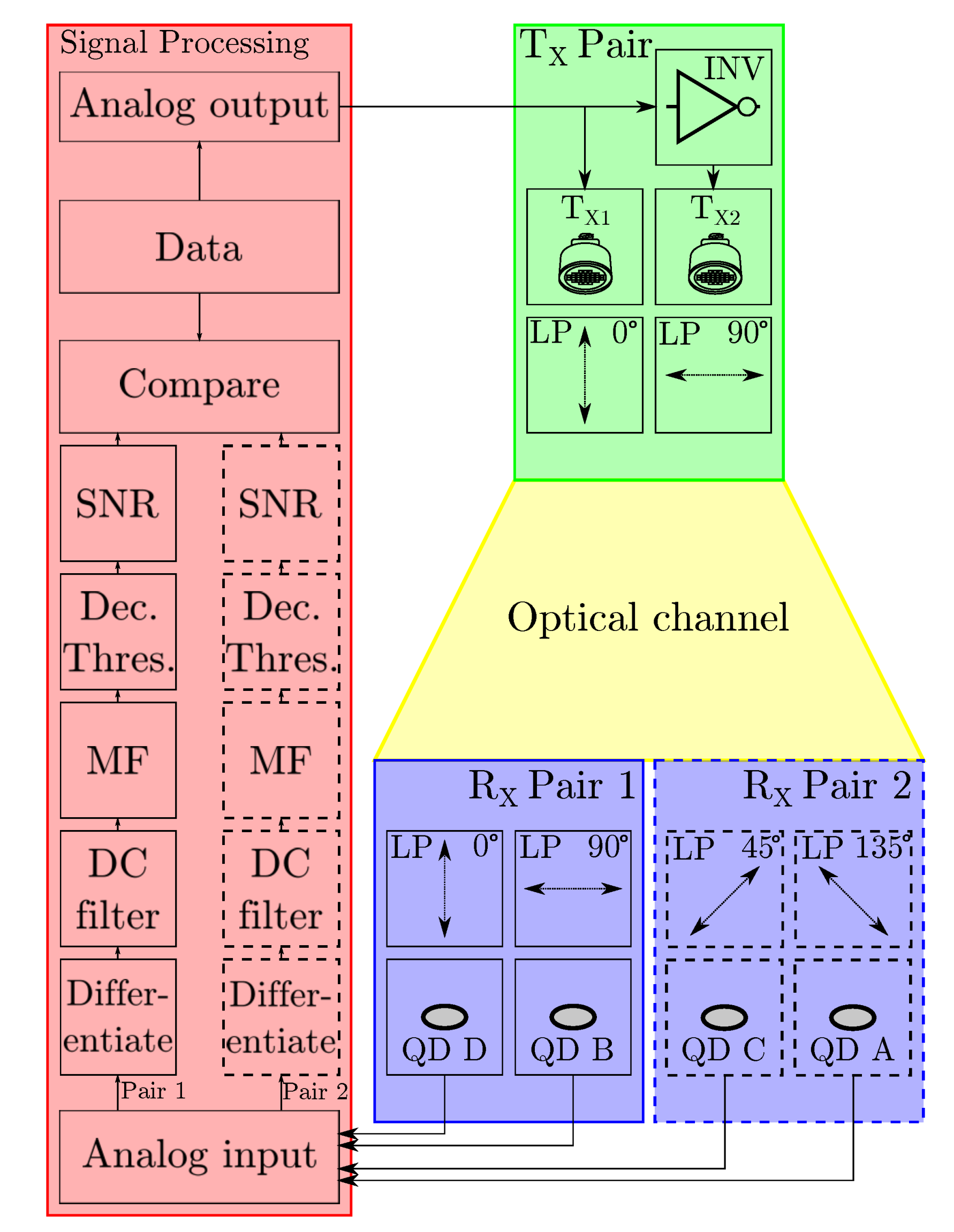
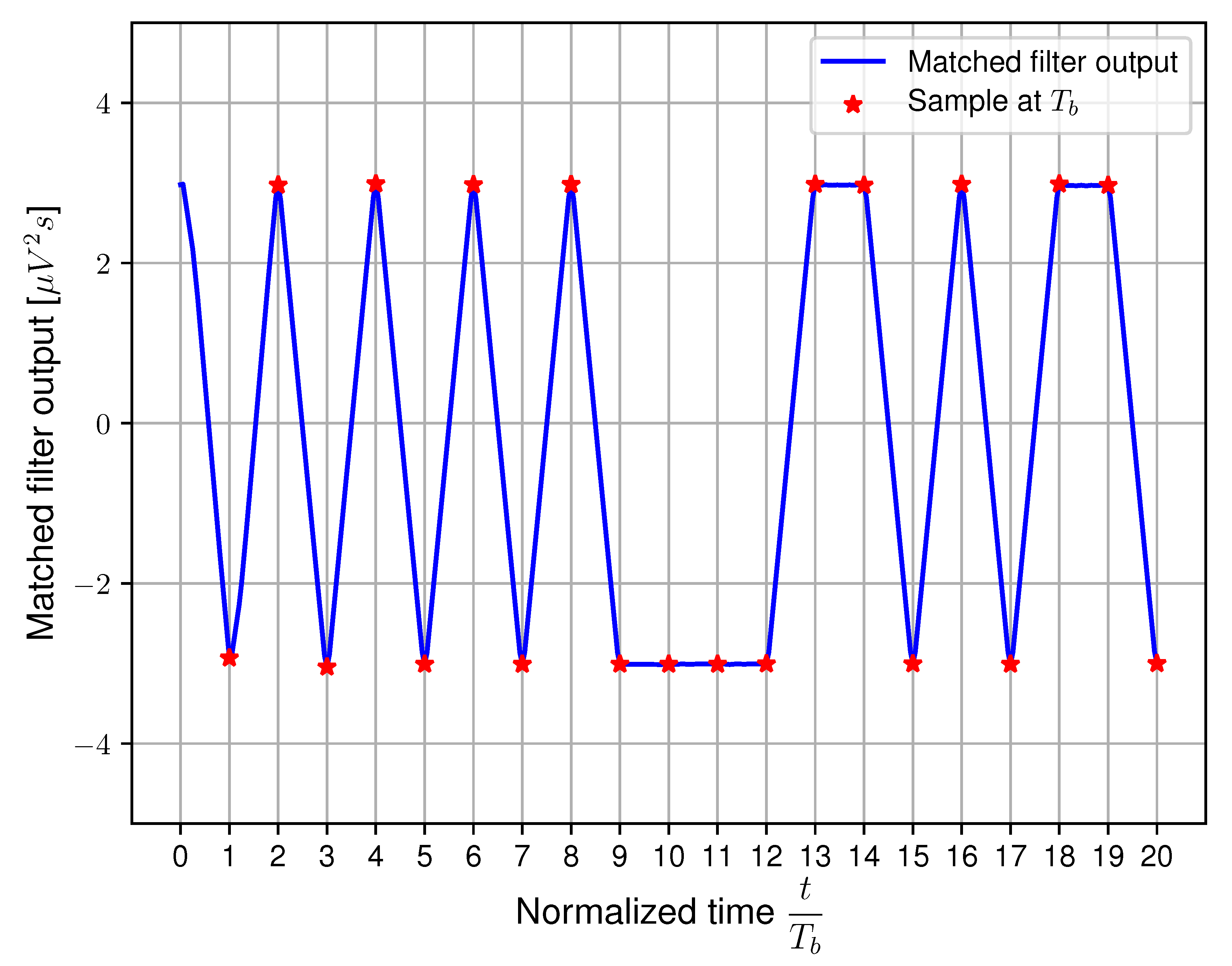
2.3. Signal Processing and Signal-to-Noise Ratio ()
3. Measurement Setup
3.1. Transmitter Side
3.2. Receiver Side
3.3. Signal Processing
4. Measurement Results
4.1. Setup A
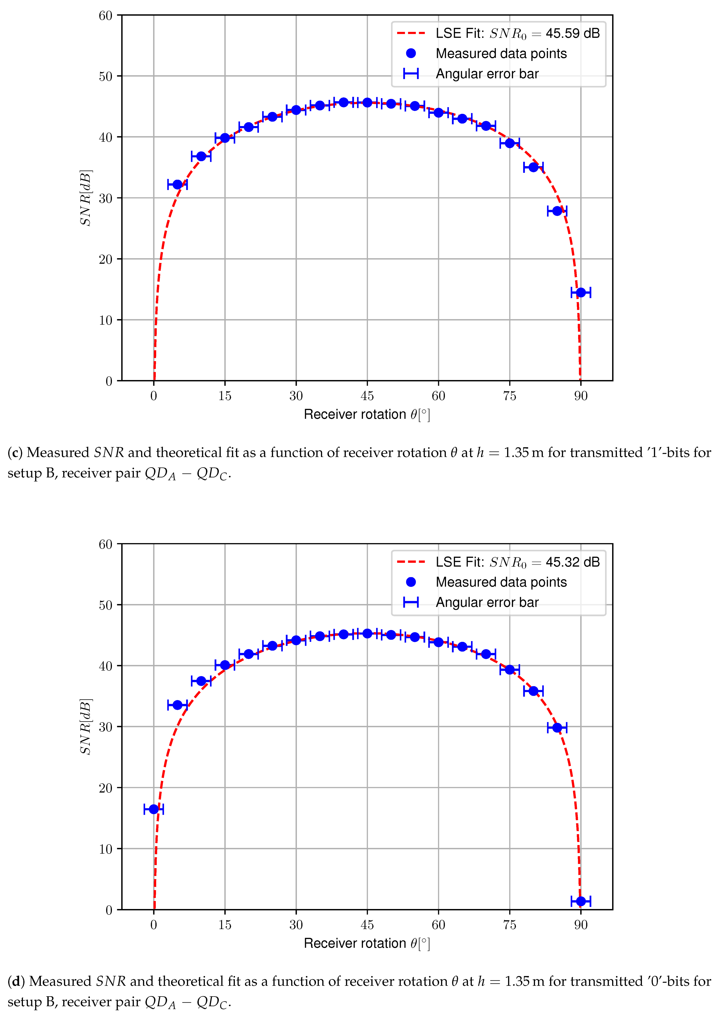
4.2. Setup B
5. Conclusions
Author Contributions
Funding
Acknowledgments
Conflicts of Interest
Abbreviations
| VLC | Visible Light Communication |
| Signal-to-Noise Ratio | |
| LED | Light-Emitting Diode |
| LC | Liquid Crystal |
| PDM | Polarization Division Multiplexing |
| OFDM | Orthogonal Frequency Division Multiplexing |
| AoA | Angle-of-Arrival |
| LP | Linear Polarizer |
| OOK | On-Off Keying |
| AWGN | Additive White Gaussian Noise |
| QD | Quadrant |
| DAQ | Data Acquisition System |
| LSE | Least Square Error |
| BER | Bit-Error Rate |
| V2V | Vehicle-to-Vehicle |
References
- Karunatilaka, D.; Zafar, F.; Kalavally, V.; Parthiban, R. LED Based Indoor Visible Light Communications: State of the Art. IEEE Commun. Surv. Tutor. 2015, 17, 1649–1678. [Google Scholar] [CrossRef]
- Pathak, P.H.; Feng, X.; Hu, P.; Mohapatra, P. Visible Light Communication, Networking, and Sensing: A Survey, Potential and Challenges. IEEE Commun. Surv. Tutor. 2015, 17, 2047–2077. [Google Scholar] [CrossRef]
- IEEE. IEEE Standard for Local and Metropolitan Area Networks–Part 15.7: Short-Range Optical Wireless Communications; IEEE Std 802.15.7-2018 (Revision of IEEE Std 802.15.7-2011); IEEE: Piscataway, NZ, USA, 2011; pp. 1–407. [Google Scholar] [CrossRef]
- Zhuang, Y.; Hua, L.; Qi, L.; Yang, J.; Cao, P.; Cao, Y.; Wu, Y.; Thompson, J.; Haas, H. A Survey of Positioning Systems Using Visible LED Lights. IEEE Commun. Surv. Tutor. 2018, 20, 1963–1988. [Google Scholar] [CrossRef] [Green Version]
- De Lausnay, S.; De Strycker, L.; Goemaere, J.; Nauwelaers, B.; Stevens, N. A survey on multiple access Visible Light Positioning. In Proceedings of the 2016 IEEE International Conference on Emerging Technologies and Innovative Business Practices for the Transformation of Societies (EmergiTech), Balaclava, Mauritius, 3–6 August 2016; pp. 38–42. [Google Scholar] [CrossRef]
- Cincotta, S.; He, C.; Neild, A.; Armstrong, J. QADA-PLUS: A Novel Two-Stage Receiver for Visible Light Positioning. In Proceedings of the 2018 International Conference on Indoor Positioning and Indoor Navigation (IPIN), Nantes, France, 24–27 September 2018; pp. 1–5. [Google Scholar] [CrossRef]
- Aparicio-Esteve, E.; Hernandez, A.; Urena, J.; Villadangos, J.M. Visible Light Positioning System Based on a Quadrant Photodiode and Encoding Techniques. IEEE Trans. Instrum. Meas. 2019, 69, 5589–5603. [Google Scholar] [CrossRef]
- Mohammed, M.; He, C.; Cincotta, S.; Neild, A.; Armstrong, J. Communication Aspects of Visible Light Positioning (VLP) Systems Using a Quadrature Angular Diversity Aperture (QADA) Receiver. Sensors 2020, 20, 1977. [Google Scholar] [CrossRef] [PubMed] [Green Version]
- Yang, Z.; Wang, Z.; Zhang, J.; Huang, C.; Zhang, Q. Polarization-Based Visible Light Positioning. IEEE Trans. Mob. Comput. 2019, 18, 715–727. [Google Scholar] [CrossRef]
- Chan, C.L.; Tsai, H.M.; Lin, K.C.J. POLI: Long-Range Visible Light Communications Using Polarized Light Intensity Modulation. In Proceedings of the 15th Annual International Conference on Mobile Systems, Applications, and Services, Niagara Falls, NY, USA, 19–23 June 2017; pp. 109–120. [Google Scholar]
- Wang, Y.; Yang, C.; Wang, Y.; Chi, N. Gigabit polarization division multiplexing in visible light communication. Opt. Lett. 2014, 39, 1823–1826. [Google Scholar] [CrossRef] [PubMed]
- Kwon, D.H.; Kim, S.J.; Yang, S.H.; Han, S.K. Optimized pre-equalization for gigabit polarization division multiplexed visible light communication. Opt. Eng. 2015, 54. [Google Scholar] [CrossRef]
- Kim, S.J.; Kwon, D.H.; Yang, S.H.; Han, S.K. Asymmetric multi-input multi-output system in visible light communication for polarization-tolerant polarization division multiplexing transmission. Opt. Eng. 2016, 55. [Google Scholar] [CrossRef]
- Chvojka, P.; Burton, A.; Pesek, P.; Li, X.; Ghassemlooy, Z.; Zvanovec, S.; Haigh, P.A. Visible light communications: Increasing data rates with polarization division multiplexing. Opt. Lett. 2020, 45, 2977–2980. [Google Scholar] [CrossRef] [PubMed]
- Wei, L.Y.; Hsu, C.W.; Chow, C.W.; Yeh, C.H. 40-Gbit/s Visible Light Communication using Polarization-Multiplexed R/G/B Laser Diodes with 2-m Free-Space Transmission. In Proceedings of the 2019 Optical Fiber Communications Conference and Exhibition (OFC), San Diego, CA, USA, 3–7 March 2019; pp. 1–3. [Google Scholar]
- Atta, M.A.; Bermak, A. A Polarization-Based Interference-Tolerant VLC Link for Low Data Rate Applications. IEEE Photonics J. 2018, 10, 1–11. [Google Scholar] [CrossRef]
- De Bruycker, J.; Raes, W.; Zvanovec, S.; Stevens, N. Influence of Receiver Orientation on Differential Polarization-based VLC. In Proceedings of the 2020 12th International Symposium on Communication Systems, Networks and Digital Signal Processing (CSNDSP) (CSNDSP2020), Porto, Portugal, 20–22 July 2020. [Google Scholar]
- Collett, E. Field Guide to Polarization; Field Guide Series; SPIE Press: Bellingham, WA, US, 2005. [Google Scholar]
- Keskin, M.F.; Gezici, S. Comparative Theoretical Analysis of Distance Estimation in Visible Light Positioning Systems. J. Light. Technol. 2016, 34, 854–865. [Google Scholar] [CrossRef]
- Kahn, J.M.; Barry, J.R. Wireless infrared communications. Proc. IEEE 1997, 85, 265–298. [Google Scholar] [CrossRef] [Green Version]
- Rahaim, M.; Little, T.D.C. Reconciling Approaches to SNR Analysis in Optical Wireless Communications. In Proceedings of the 2017 IEEE Wireless Communications and Networking Conference (WCNC), Las Vegas, NV, USA, 19–22 March 2017; pp. 1–6. [Google Scholar]
- Guimaraes, D. Digital Transmission; Signals and Communication Technology; Springer: Berlin/Heidelberg, Germany, 2009. [Google Scholar]


| Setup A | Setup B | |
|---|---|---|
| Photodetector | Thorlabs PDA36A2 | Hamamatsu S5981 |
| Active Area | 2 × | 4 × |
| Peak Responsitivity | / | / |
| Transimpedance Gain | 27 | |
| DC Bias | ||
| DAQ | National Instruments USB-6215 | National Instruments USB-6212 |
| Data rate | 4 kbps | 4 kbps |
| Sample rate | ||
| ADC input range | ||
| ADC resolution | 16 bit | 16 bit |
© 2020 by the authors. Licensee MDPI, Basel, Switzerland. This article is an open access article distributed under the terms and conditions of the Creative Commons Attribution (CC BY) license (http://creativecommons.org/licenses/by/4.0/).
Share and Cite
De Bruycker, J.; Raes, W.; Zvánovec, S.; Stevens, N. Polarization Differential Visible Light Communication: Theory and Experimental Evaluation. Sensors 2020, 20, 5661. https://doi.org/10.3390/s20195661
De Bruycker J, Raes W, Zvánovec S, Stevens N. Polarization Differential Visible Light Communication: Theory and Experimental Evaluation. Sensors. 2020; 20(19):5661. https://doi.org/10.3390/s20195661
Chicago/Turabian StyleDe Bruycker, Jorik, Willem Raes, Stanislav Zvánovec, and Nobby Stevens. 2020. "Polarization Differential Visible Light Communication: Theory and Experimental Evaluation" Sensors 20, no. 19: 5661. https://doi.org/10.3390/s20195661