Analysis of the Variability in Soil Moisture Measurements by Capacitance Sensors in a Drip-Irrigated Orchard

 , , ,
, , , 
Abstract
:1. Introduction
2. Materials and Methods
2.1. Experimental Orchard
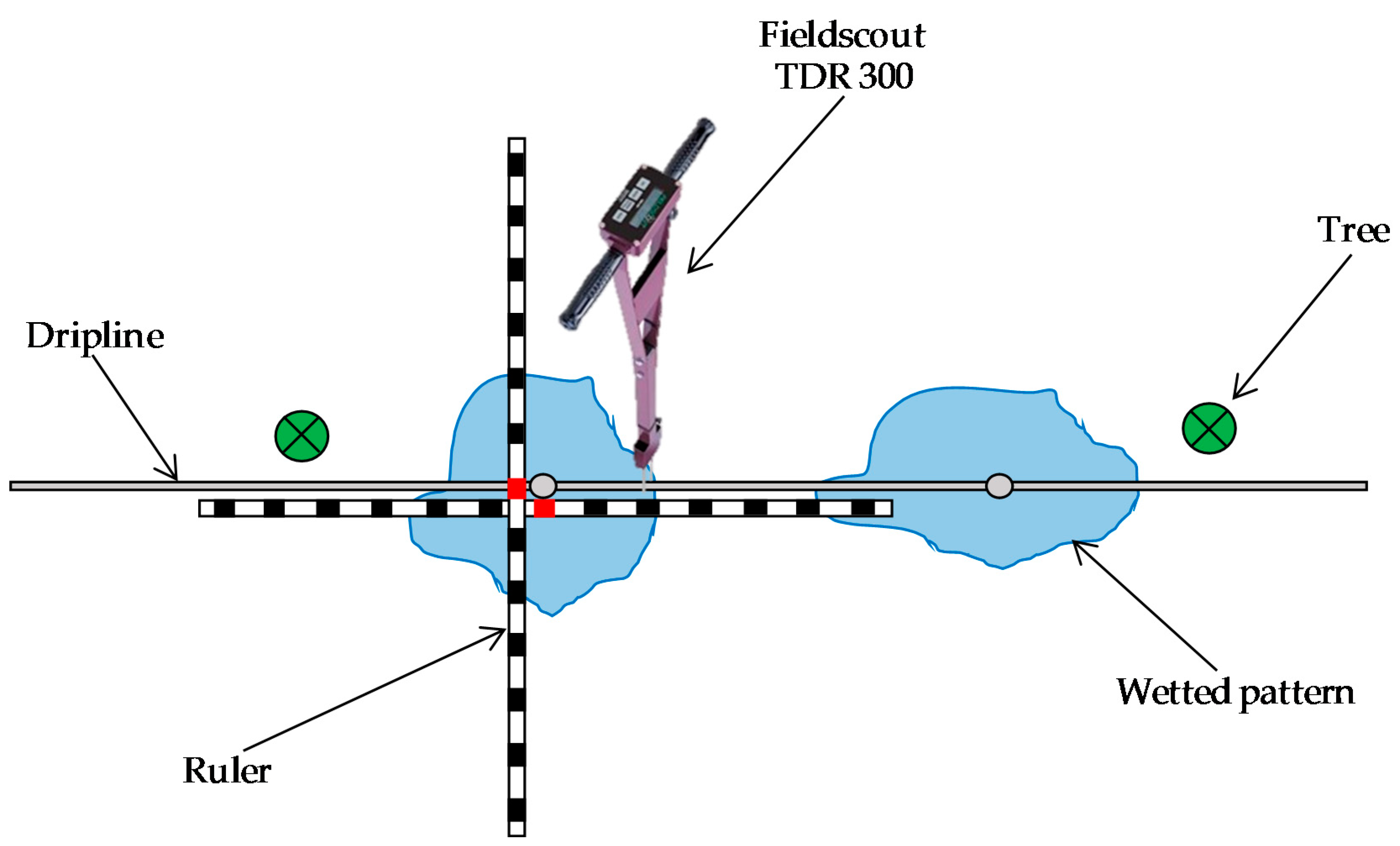
2.2. Soil Water Content Measurements
2.3. HYDRUS-3D Model
2.4. Analysis of Sensor Performance
- -
- Repeatability between sensors: refers to the variability between sensors installed at equivalent depth and position relative to the dripper. They were quantified as the root mean square error (RMSE) between those repetitions, using the dataset composed of the daily values of Plot I and Plot II in 2017 and 2018. In the case of the HYDRUS-3D simulations, the repetitions came from the 3 virtual sensors defined for each of the 10 locations of interest.
- -
- Sensitivity to the soil water balance: refers to the dependence of the SWC at a given sensor location on the balance of water inputs/outputs to the soil. This indicator was quantified through a regression that modelled the sensor measurement of any given day as a function of the sensor measurement 7 days earlier, the balance that day, and the aggregated balance of the previous 7 days.
- -
- SWCdd: the driest SWC measured by the sensor on day d, cm3 cm−3.
- -
- SWCdd−7: the driest SWC measured by the sensor 7 days earlier (d − 7), cm3 cm−3.
- -
- bald: the balance of water inputs and outputs (DIDd + PPTd – ETd), mm.
- -
- DIDd: the daily irrigation dose on day d, mm.
- -
- PPTd: the daily rainfall dose on day d, mm.
- -
- ETd: the daily irrigation dose on day d, mm.
- -
- Σbald-7...d: the aggregated balance of water inputs and outputs in the previous 7 days (Σ(DIDd + PPTd – ETd)), mm.
- -
- Coef0, Coef1, and Coef2: the regression coefficients.
2.5. Statistical Calculations
3. Results
3.1. Variability in the Soil Conditions around a Dripper
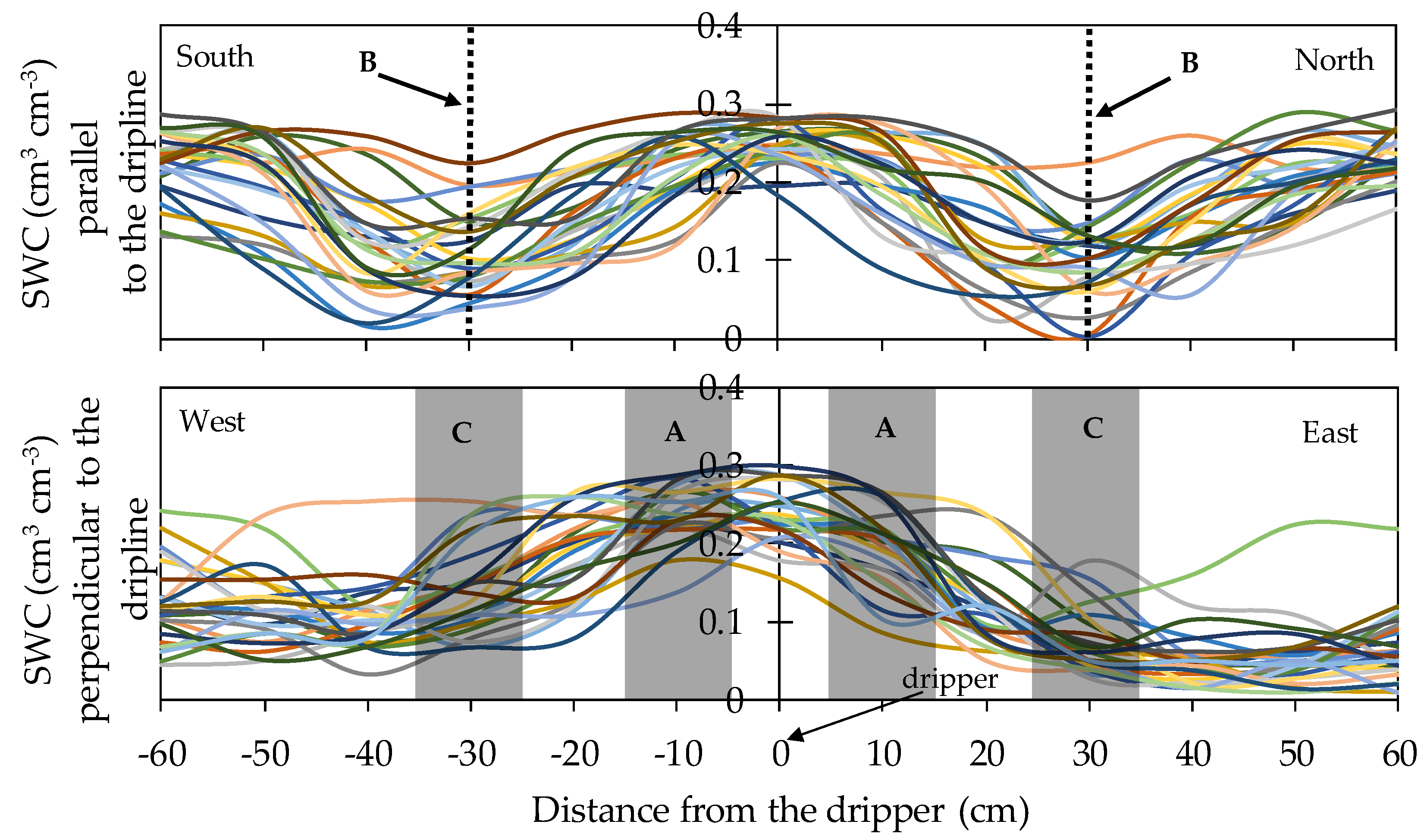
3.1.1. Centering and Extent of the Wetted Area
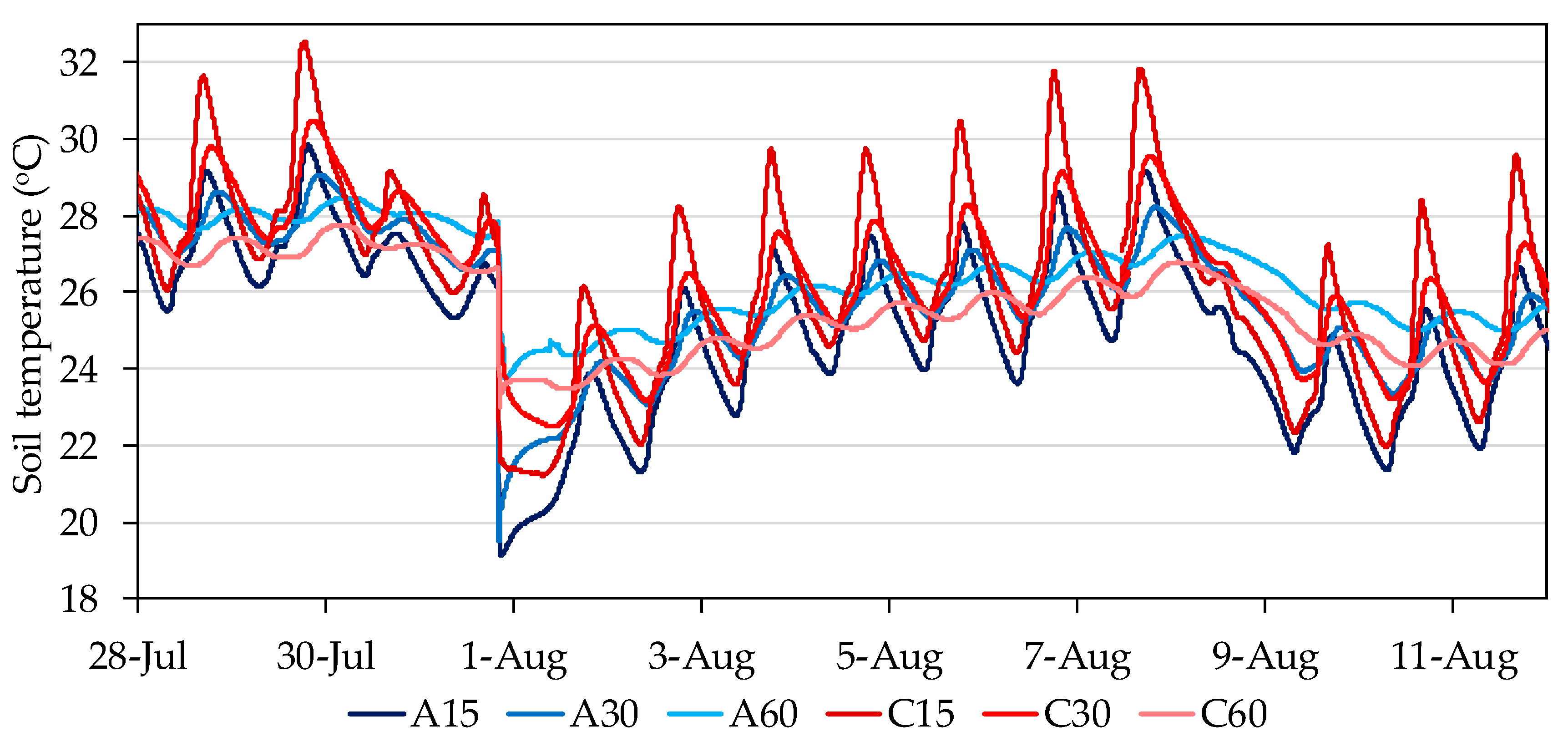
3.1.2. Pattern of Temperature in a Soil Wet Bulb
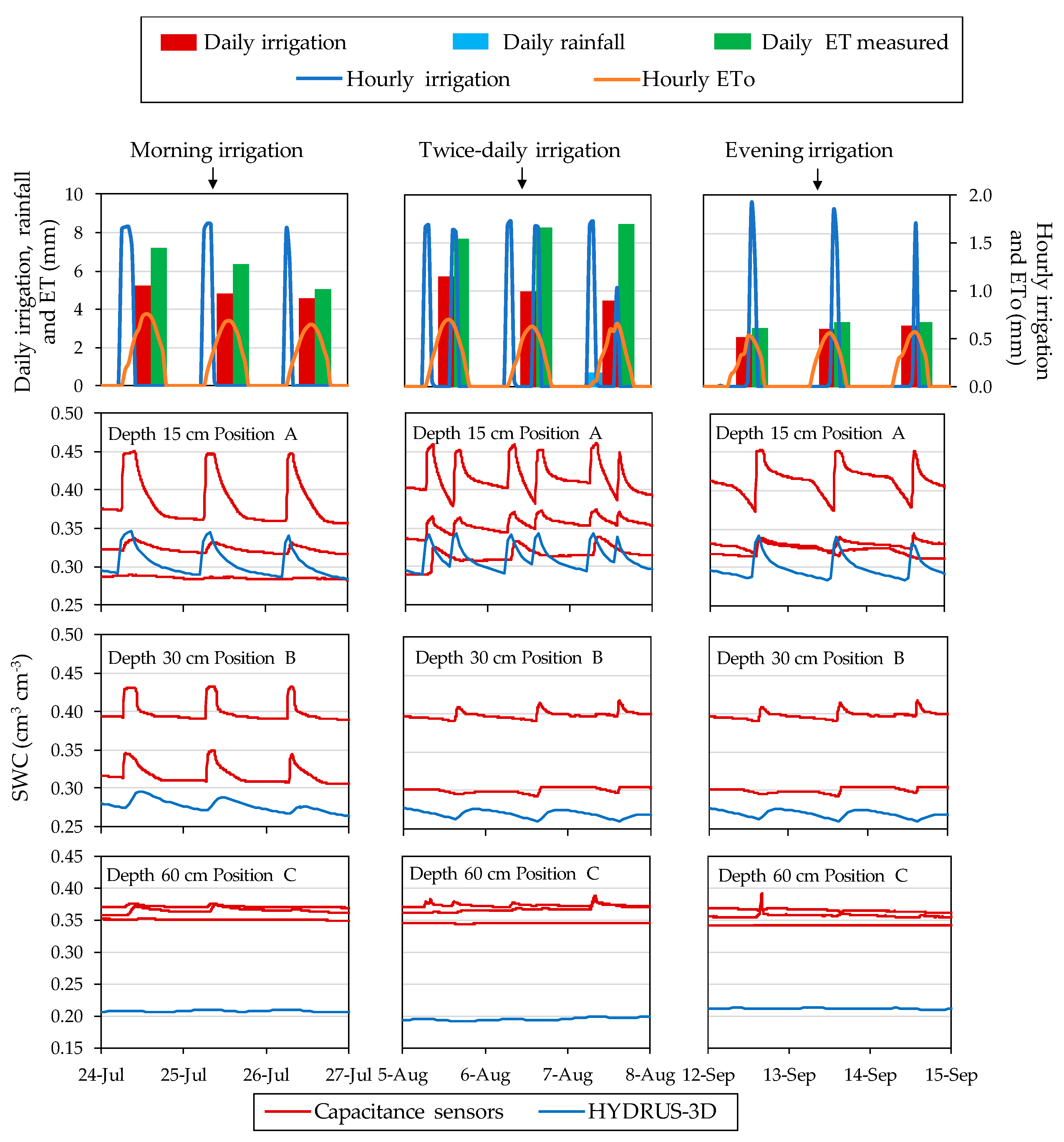
3.2. Overall Response of the Sensors
3.3. Variability between Sensors at Seasonal Scale
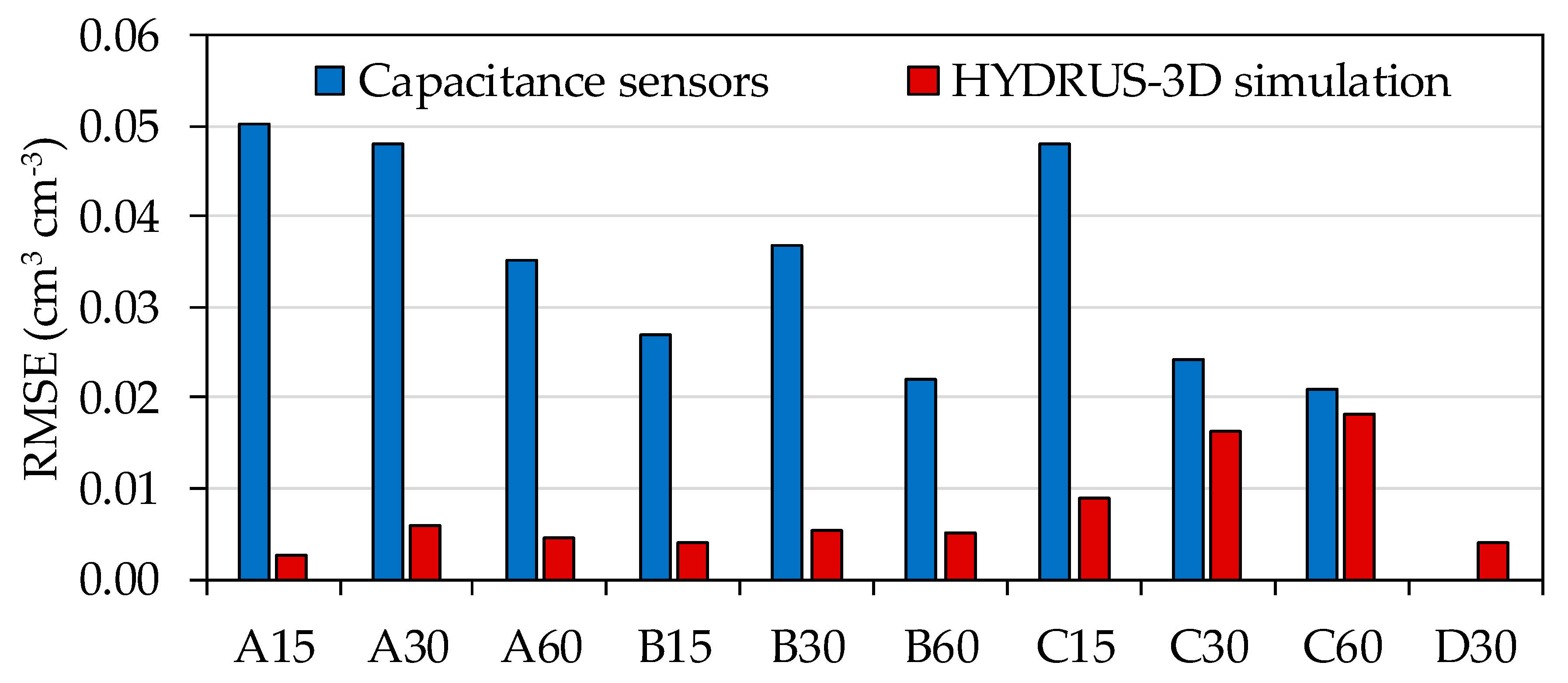
Repeatability between Sensors
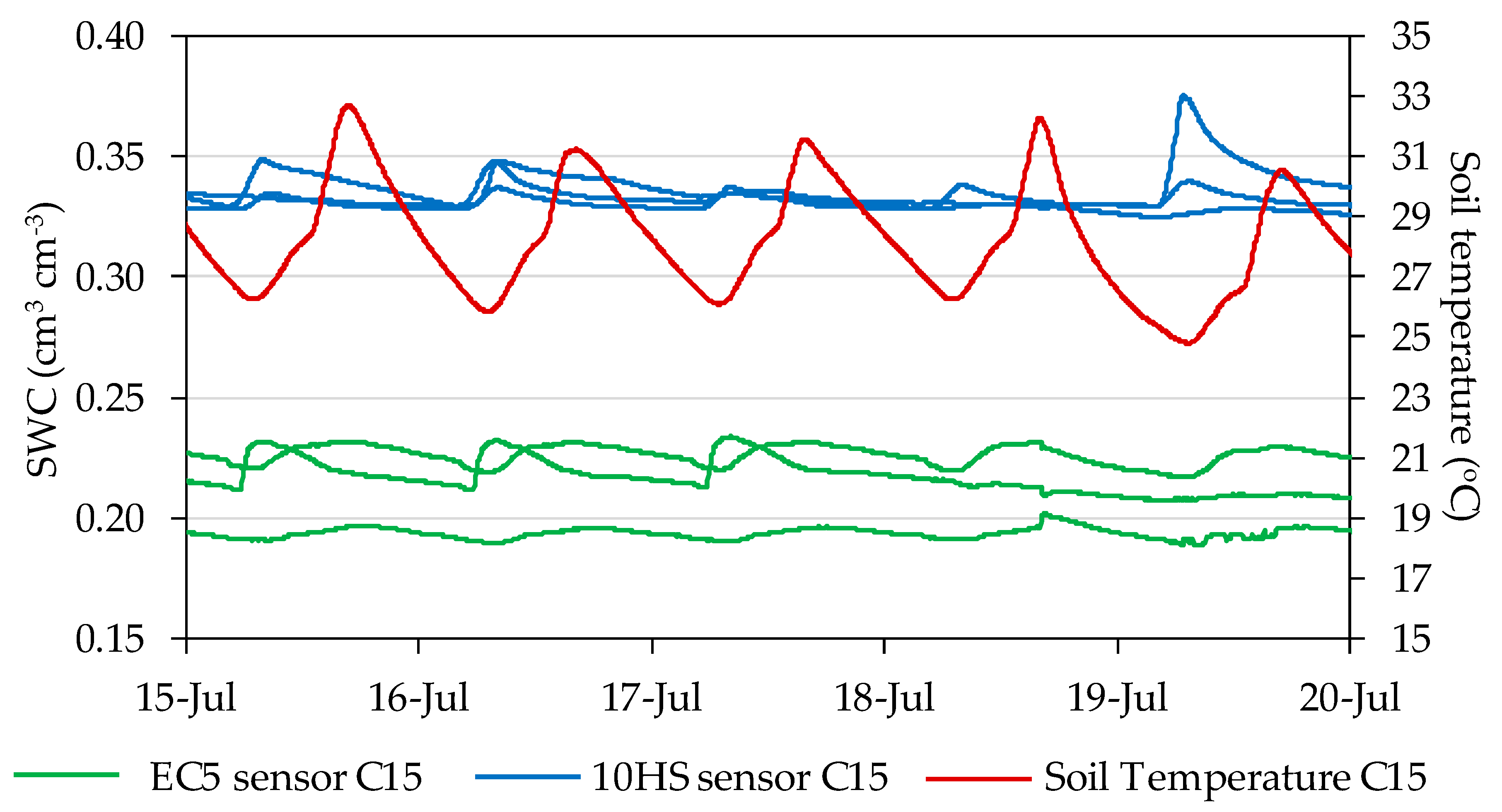
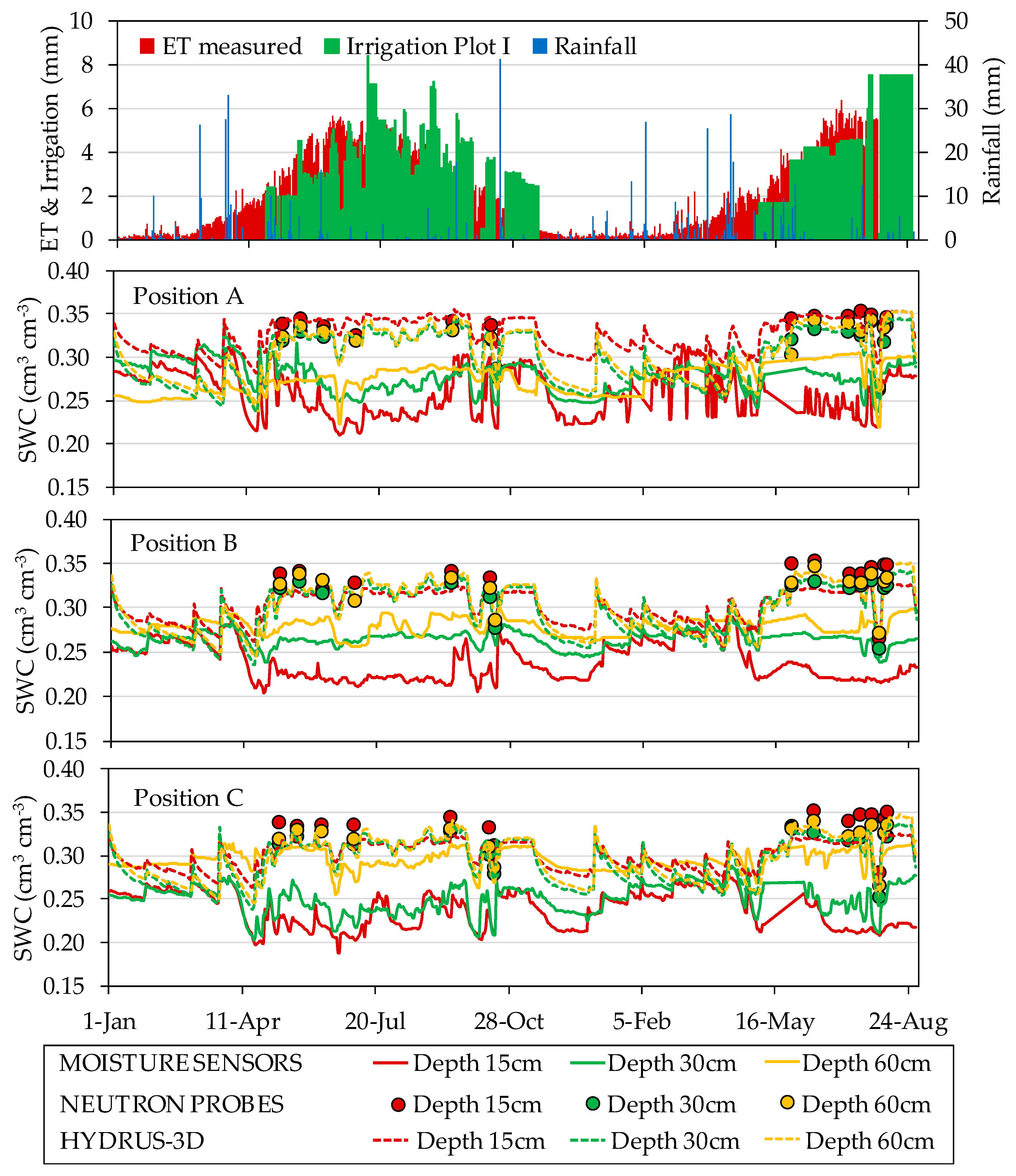
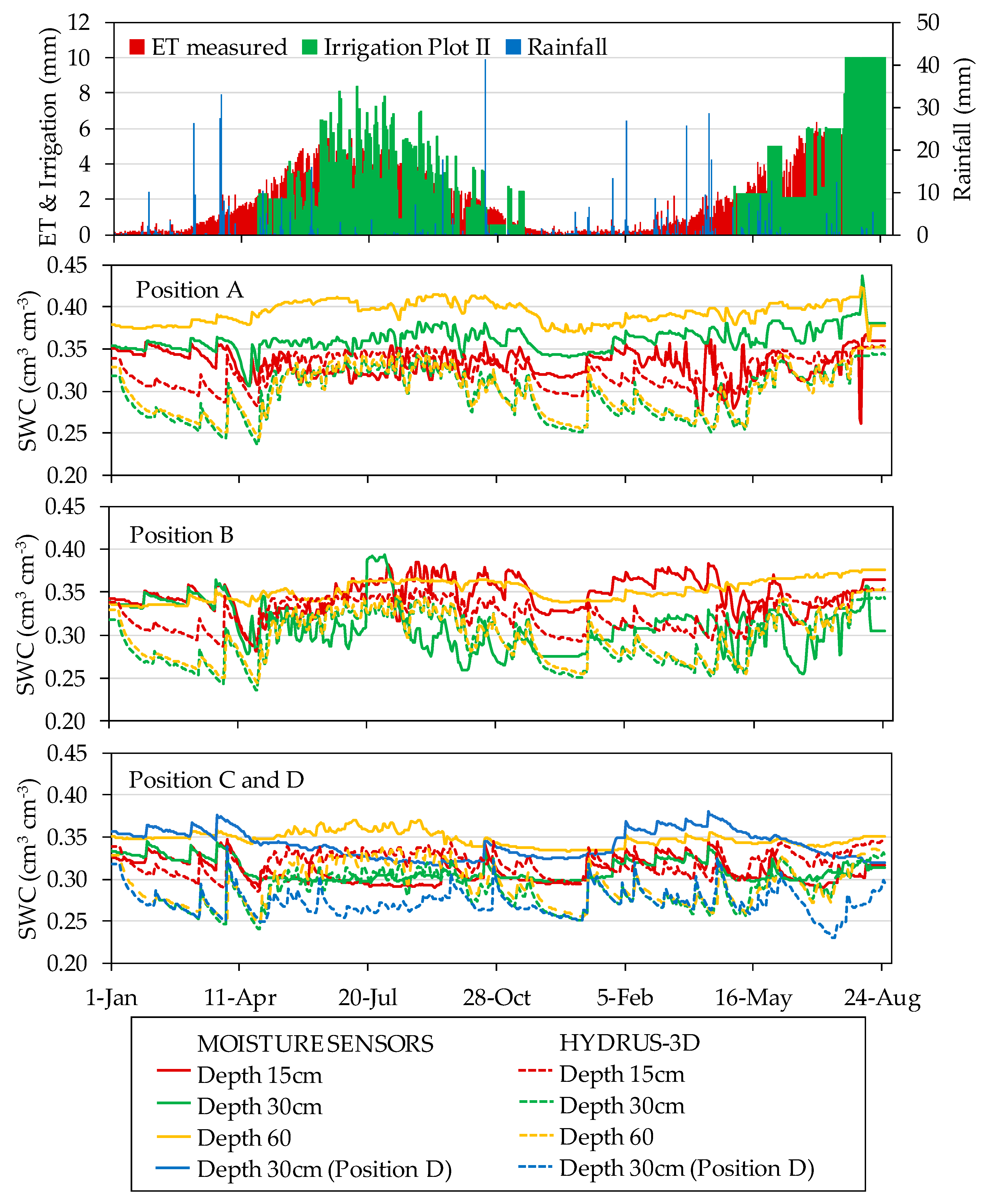
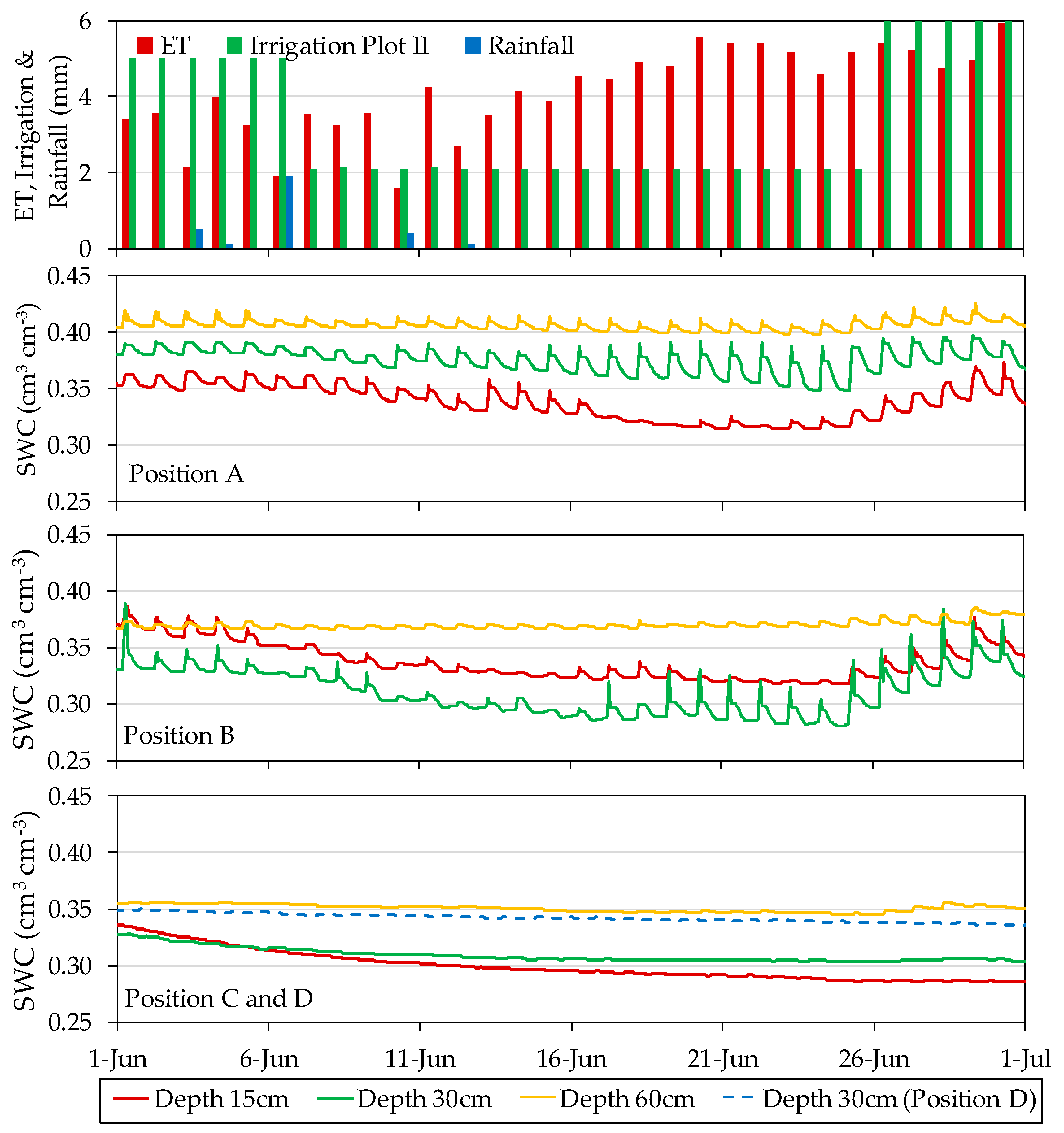
3.4. Seasonal Pattern at Each Sensor Location in the Soil
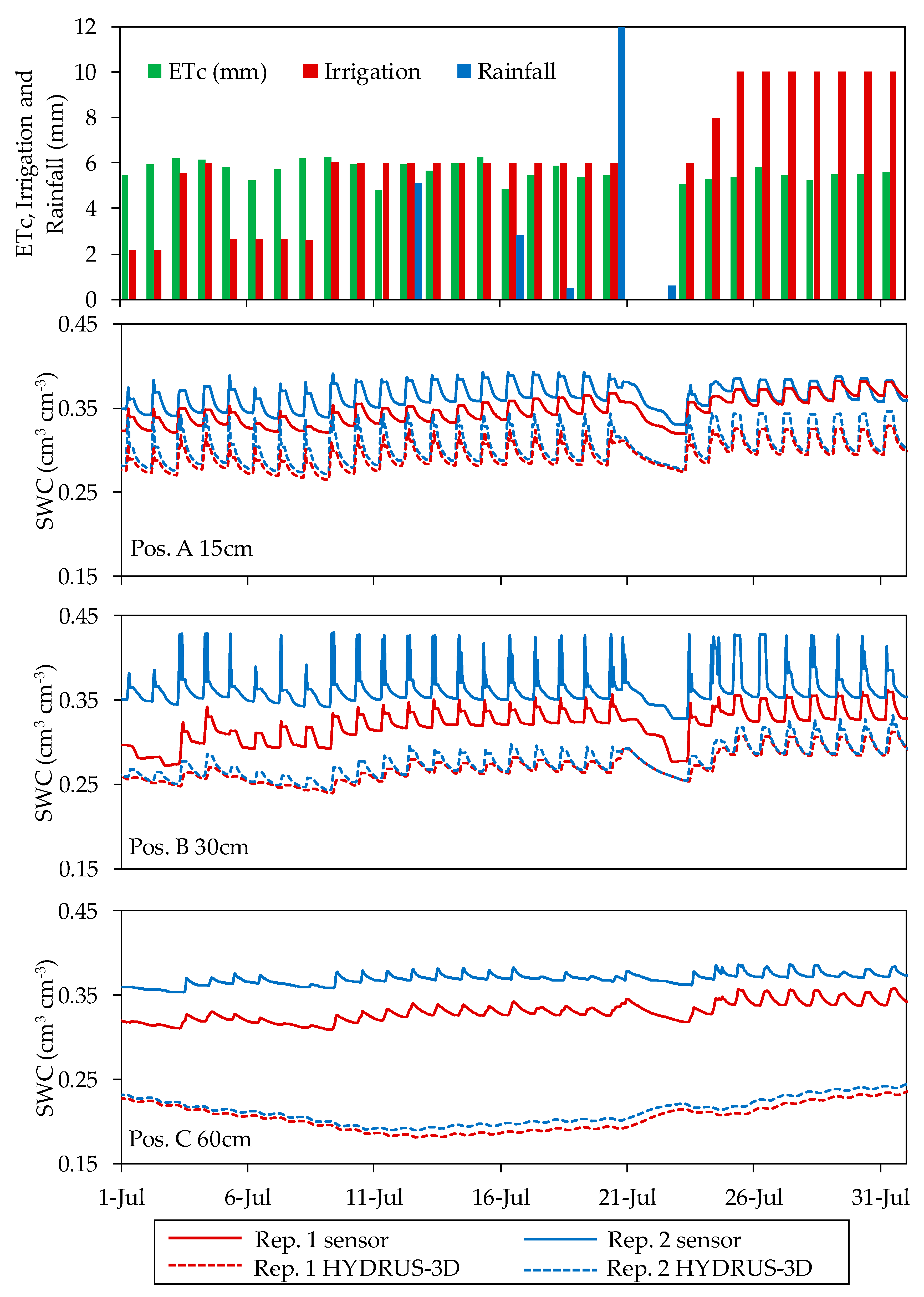
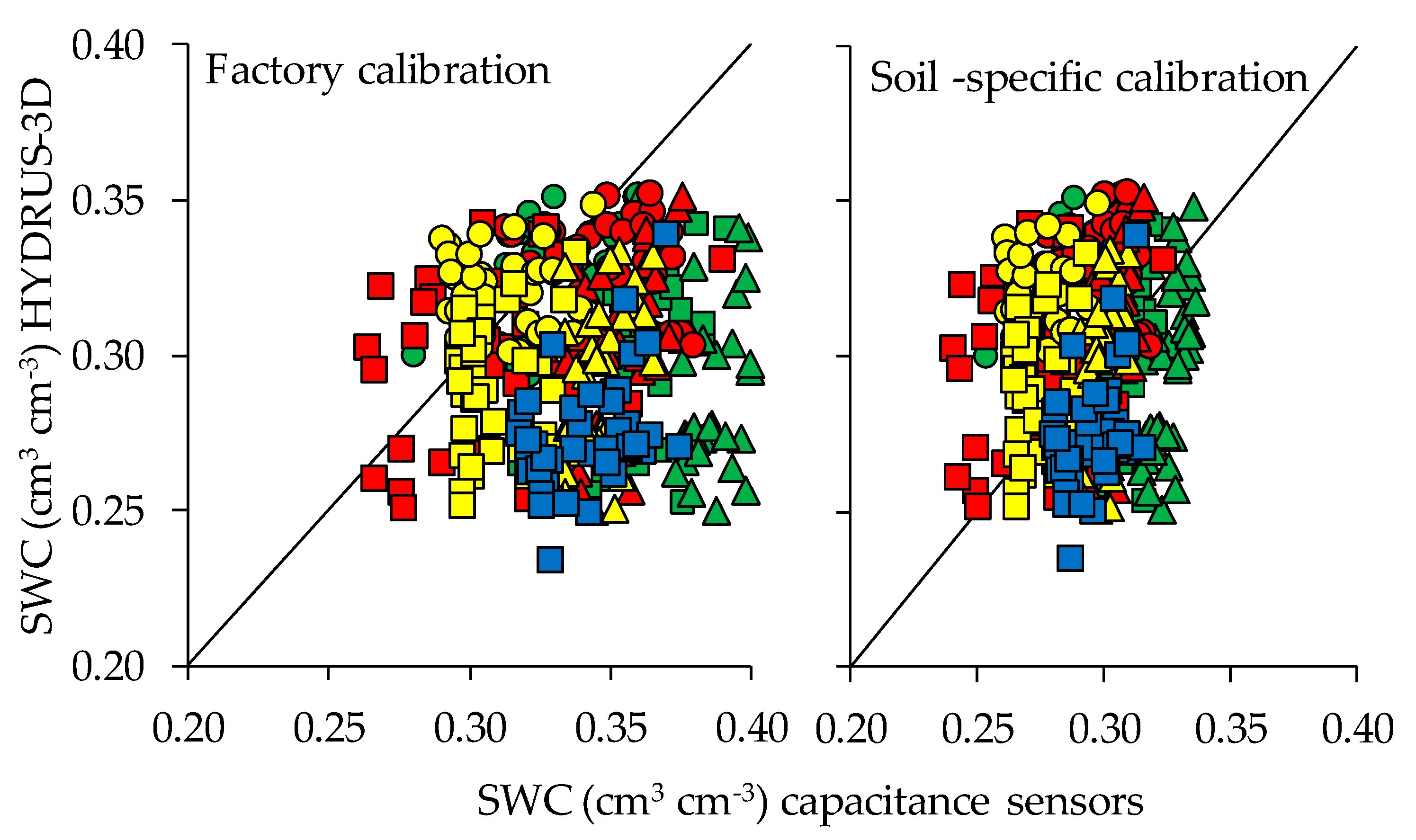
3.5. Comparisons between Capacitance Sensor Measurements and HYDRUS-3D Simulations
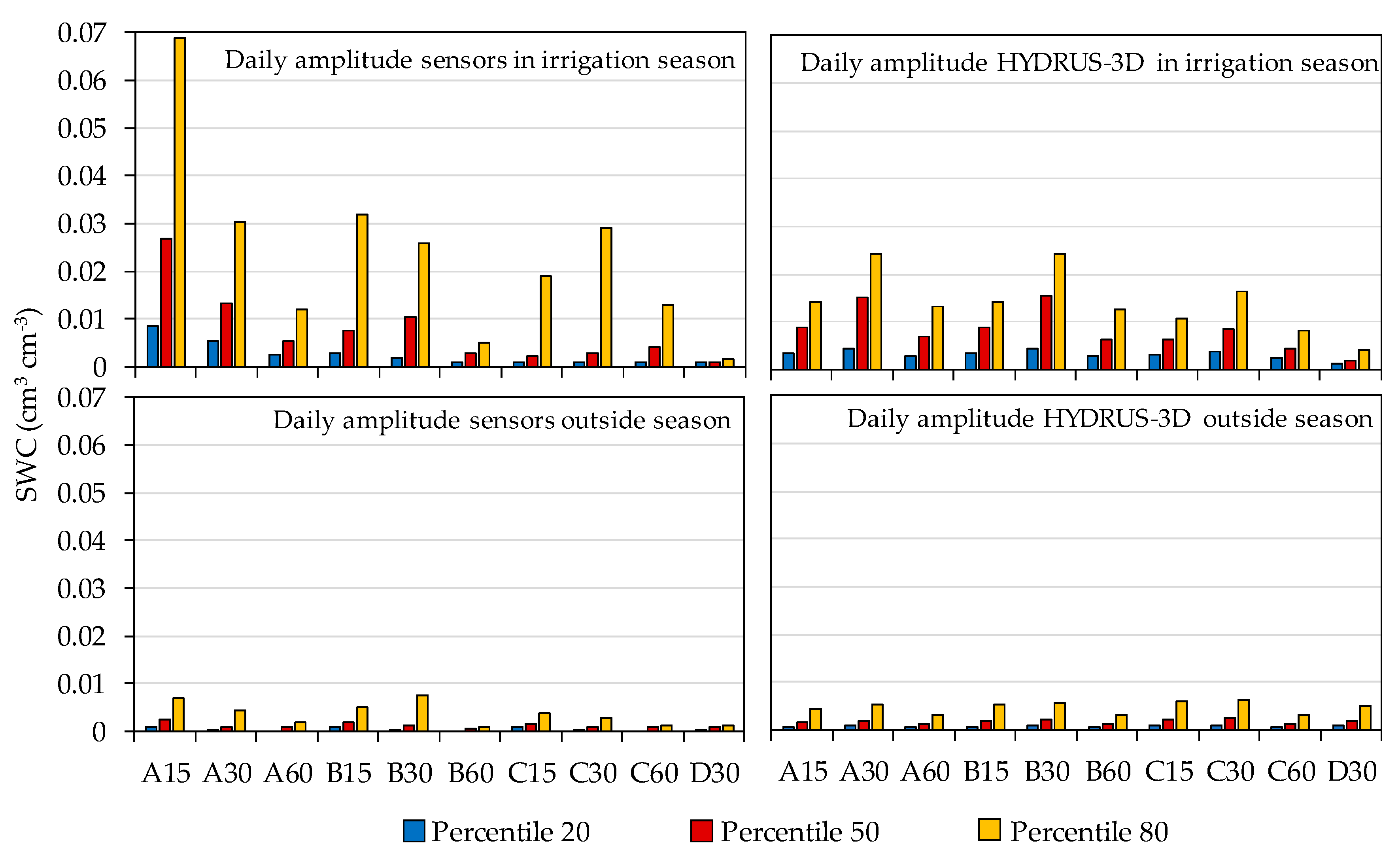
3.6. Sensor Sensitivity at Each Location to Fluctuations in the Balance of Water Inputs/Outputs
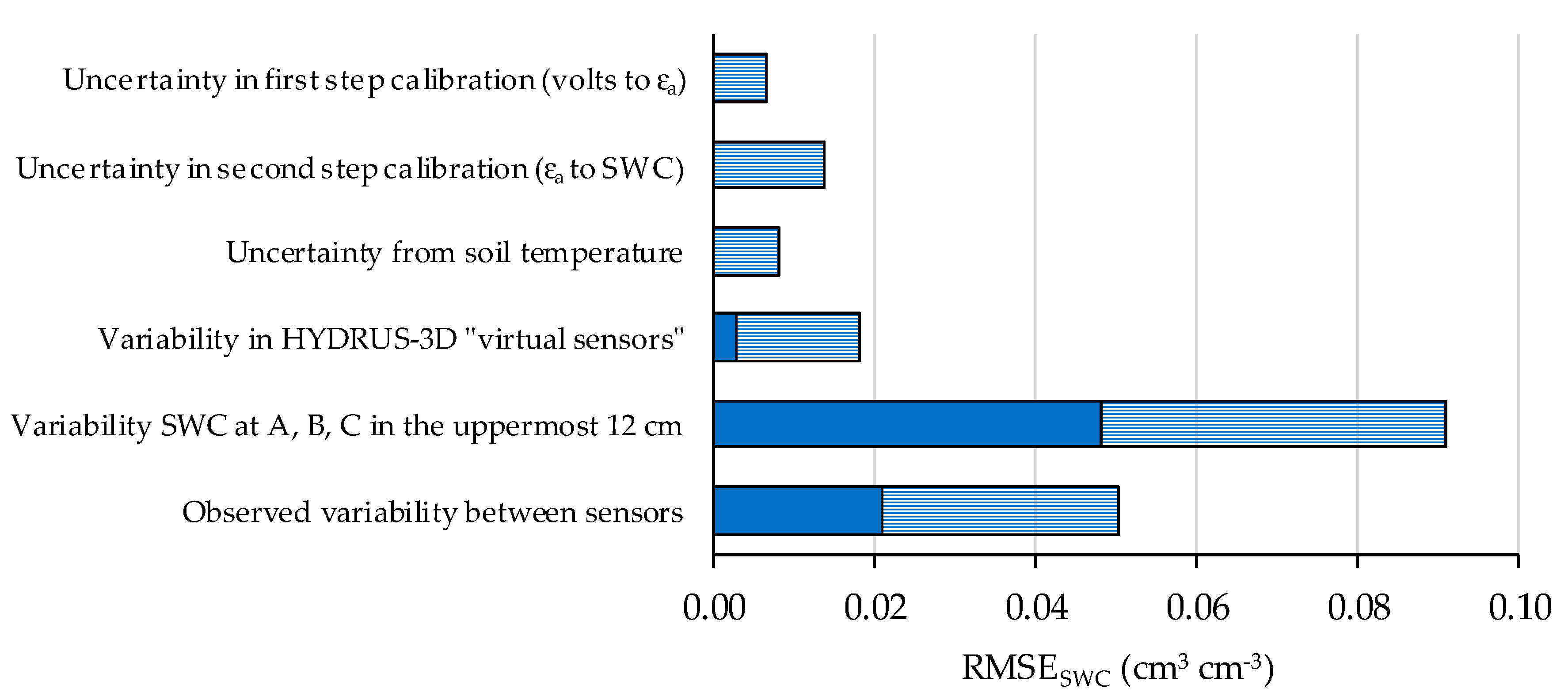
3.7. Components of the Variability in the Measurements by Capacitive-Type Soil Sensors
4. Discussion
4.1. Variability in the Soil Conditions
4.2. Repeatability between Sensors
4.3. Sensor Sensitivity at Each Location
4.4. Contributions of Different Factors to Sensor-To-Sensor Differences
4.5. Recommended Location for Capacitance Sensors in Drip Irrigation
5. Conclusions
Author Contributions
Funding
Acknowledgments
Conflicts of Interest
References
- Ashofteh, P.-S.; Bozorg-Haddad, O.; Akbari-Alashti, H.; Mariño, M.A. Determination of Irrigation Allocation Policy under Climate Change by Genetic Programming. J. Irrig. Drain. Eng. 2015, 141, 04014059. [Google Scholar] [CrossRef] [Green Version]
- Kilic, M. A new analytical method for estimating the 3D volumetric wetting pattern under drip irrigation system. Agric. Water Manag. 2020, 228, 105898. [Google Scholar] [CrossRef]
- Rajput, T.; Patel, N. Water and nitrate movement in drip-irrigated onion under fertigation and irrigation treatments. Agric. Water Manag. 2006, 79, 293–311. [Google Scholar] [CrossRef]
- Liao, L.; Zhang, L.; Bengtsson, L. Soil moisture variation and water consumption of spring wheat and their effects on crop yield under drip irrigation. Irrig. Drain. Syst. 2008, 22, 253–270. [Google Scholar] [CrossRef]
- Naglič, B.; Kechavarzi, C.; Coulon, F.; Pintar, M. Numerical investigation of the influence of texture, surface drip emitter discharge rate and initial soil moisture condition on wetting pattern size. Irrig. Sci. 2014, 32, 421–436. [Google Scholar] [CrossRef]
- Arraes, F.D.D.; De Miranda, J.H.; Duarte, S.N. Modeling Soil Water Redistribution under Surface Drip Irrigation. Eng. Agrícola 2019, 39, 55–64. [Google Scholar] [CrossRef] [Green Version]
- Hao, A.; Marui, A.; Haraguchi, T.; Nakano, Y. Estimation of wet bulb formation in various soil during drip irrigation. J. Fac. Agric. Kyushu Univ. 2007, 52, 187. [Google Scholar]
- Kandelous, M.M.; Šimůnek, J.; Van Genuchten, M.; Malek, K. Soil Water Content Distributions between Two Emitters of a Subsurface Drip Irrigation System. Soil Sci. Soc. Am. J. 2011, 75, 488–497. [Google Scholar] [CrossRef]
- Nolz, R.; Loiskandl, W. Evaluating soil water content data monitored at different locations in a vineyard with regard to irrigation control. Soil Water Res. 2017, 12, 152–160. [Google Scholar] [CrossRef] [Green Version]
- Soulis, K.X.; Elmaloglou, S. Optimum soil water content sensors placement for surface drip irrigation scheduling in layered soils. Comput. Electron. Agric. 2018, 152, 1–8. [Google Scholar] [CrossRef]
- Ledieu, J.; De Ridder, P.; De Clerck, P.; Dautrebande, S. A method of measuring soil moisture by time-domain reflectometry. J. Hydrol. 1986, 88, 319–328. [Google Scholar] [CrossRef]
- Zotarelli, L.; Dukes, M.D.; Scholberg, J.M.S.; Femminella, K.; Munoz-Carpena, R. Irrigation Scheduling for Green Bell Peppers Using Capacitance Soil Moisture Sensors. J. Irrig. Drain. Eng. 2011, 137, 73–81. [Google Scholar] [CrossRef]
- Cummings, R.W.; Chandler, R.F. A Field Comparison of the Electrothermal and Gypsum Block Electrical Resistance Methods with the Tensiometer Method for Estimating Soil Moisture in Situ. Soil Sci. Soc. Am. J. 1941, 5, 80–85. [Google Scholar] [CrossRef]
- Chanasyk, D.S.; Naeth, M.A. Field measurement of soil moisture using neutron probes. Can. J. Soil Sci. 1996, 76, 317–323. [Google Scholar] [CrossRef]
- Munoz-Carpena, R.; Li, Y.; Klassen, W.; Dukes, M.D. Field Comparison of Tensiometer and Granular Matrix Sensor Automatic Drip Irrigation on Tomato. HortTechnology 2005, 15, 584–590. [Google Scholar] [CrossRef] [Green Version]
- Kojima, Y.; Shigeta, R.; Miyamoto, N.; Shirahama, Y.; Nishioka, K.; Mizoguchi, M.; Kawahara, Y. Low-Cost Soil Moisture Profile Probe Using Thin-Film Capacitors and a Capacitive Touch Sensor. Sensors 2016, 16, 1292. [Google Scholar] [CrossRef]
- Bogena, H.R.; Huisman, J.A.; Schilling, B.; Weuthen, A.; Vereecken, H. Effective Calibration of Low-Cost Soil Water Content Sensors. Sensors 2017, 17, 208. [Google Scholar] [CrossRef] [Green Version]
- Jones, S.B.; Blonquist, J.M.; Robinson, D.A.; Rasmussen, V.P.; Or, D. Standardizing Characterization of Electromagnetic Water Content Sensors: Part 1. Methodology. Vadose Zone J. 2005, 4, 1048–1058. [Google Scholar] [CrossRef] [Green Version]
- Spelman, D.; Kinzli, K.-D.; Kunberger, T. Calibration of the 10HS Soil Moisture Sensor for Southwest Florida Agricultural Soils. J. Irrig. Drain. Eng. 2013, 139, 965–971. [Google Scholar] [CrossRef]
- Visconti, F.; De Paz, J.M.; Martínez, D.; Molina, M.J. Laboratory and field assessment of the capacitance sensors Decagon 10HS and 5TE for estimating the water content of irrigated soils. Agric. Water Manag. 2014, 132, 111–119. [Google Scholar] [CrossRef]
- Rosenbaum, U.; Huisman, J.A.; Vrba, J.; Vereecken, H.; Bogena, H.R. Correction of Temperature and Electrical Conductivity Effects on Dielectric Permittivity Measurements with ECH2 O Sensors. Vadose Zone J. 2011, 10, 582–593. [Google Scholar] [CrossRef]
- Fares, A.; Alva, A.K. Evaluation of capacitance probes for optimal irrigation of citrus through soil moisture monitoring in an entisol profile. Irrig. Sci. 2000, 19, 57–64. [Google Scholar] [CrossRef]
- Gallardo, M.; Elia, A.; Thompson, R.B. Decision support systems and models for aiding irrigation and nutrient management of vegetable crops. Agric. Water Manag. 2020, 240, 106209. [Google Scholar] [CrossRef]
- Rosenbaum, U.; Huisman, J.A.; Weuthen, A.; Vereecken, H.; Bogena, H.R. Sensor-to-sensor variability of the ECH2O EC-5, TE, and 5TE sensors in dielectric liquids. Vadose Zone J. 2010, 9, 181–186. [Google Scholar] [CrossRef]
- Cobos, D. 10HS Volume of Sensitivity; Application Note 13900-01; Decagon Devices: Pullman, WA, USA, 2008. [Google Scholar]
- Sakaki, T.; Limsuwat, A.; Smits, K.M.; Illangasekare, T.H. Empirical two-point α -mixing model for calibrating the ECH2 O EC-5 soil moisture sensor in sands. Water Resour. Res. 2008, 44, 44. [Google Scholar] [CrossRef]
- Waugh, W.J.; Baker, D.A.; Kastens, M.K.; Abraham, J.A. Calibration precision of capacitance and neutron soil water content gauges in arid soils. Arid. Soil Res. Rehabil. 1996, 10, 391–401. [Google Scholar] [CrossRef]
- Dane, J.H.; Hopmans, J.W. Water retention and storage. In Methods of Soil Analysis; Part 4, SSSA Book Series No. 5; Dane, J.H., Topp, G.C., Eds.; Soil Science Society of America Journal: Madison, WI, USA, 2002. [Google Scholar]
- Adla, S.; Rai, N.K.; Karumanchi, H.S.; Tripathi, S.; Disse, M.; Pande, S. Laboratory Calibration and Performance Evaluation of Low-Cost Capacitive and Very Low-Cost Resistive Soil Moisture Sensors. Sensors 2020, 20, 363. [Google Scholar] [CrossRef] [Green Version]
- Scudiero, E.; Berti, A.; Teatini, P.; Morari, F. Simultaneous Monitoring of Soil Water Content and Salinity with a Low-Cost Capacitance-Resistance Probe. Sensors 2012, 12, 17588–17607. [Google Scholar] [CrossRef] [Green Version]
- Šimůnek, J.; Van Genuchten, M.; Šejna, M. Recent Developments and Applications of the HYDRUS Computer Software Packages. Vadose Zone J. 2016, 15, 25. [Google Scholar] [CrossRef] [Green Version]
- Badni, N.; Hamoudi, S.; Alazba, A.A.; Elnesr, M.N. Simulations of Soil Moisture Distribution Patterns between Two Simultaneously-Working Surface Drippers Using Hydrus-2D/3D Model. Int. J. Eng. Technol. 2018, 10, 586–595. [Google Scholar] [CrossRef] [Green Version]
- Fan, Y.-W.; Huang, N.; Zhang, J.; Zhao, T. Simulation of Soil Wetting Pattern of Vertical Moistube-Irrigation. Water 2018, 10, 601. [Google Scholar] [CrossRef] [Green Version]
- Skaggs, T.H.; Trout, T.J.; Šimunek, J.; Shouse, P.J. Comparison of HYDRUS-2D Simulations of Drip Irrigation with Experimental Observations. J. Irrig. Drain. Eng. 2004, 130, 304–310. [Google Scholar] [CrossRef]
- Abou Lila, T.S.; Balah, M.I.; Hamed, Y.A. Solute infiltration and spatial salinity distribution behavior for the main soil types at El-Salam Canal project cultivated land. Port Said Eng. Res. J. 2005, 9, 242–253. [Google Scholar]
- Morillo, J.G.; Díaz, J.A.R.; Camacho, E.; Montesinos, P. Drip Irrigation Scheduling Using Hydrus 2-D Numerical Model Application for Strawberry Production in South-West Spain. Irrig. Drain. 2017, 66, 797–807. [Google Scholar] [CrossRef]
- Domínguez-Niño, J.M.; Arbat, G.; Raij-Hoffman, I.; Kisekka, I.; Girona, J.; Casadesús, J. Parameterization of Soil Hydraulic Parameters for HYDRUS-3D Simulation of Soil Water Dynamics in a Drip-Irrigated Orchard. Water 2020, 12, 1858. [Google Scholar] [CrossRef]
- Millán, S.; Torres, M.D.; Torres, M.D.; Moñino, M.J.; Prieto, M.H.; Moñino, J.; Prieto, M. Using Soil Moisture Sensors for Automated Irrigation Scheduling in a Plum Crop. Water 2019, 11, 2061. [Google Scholar] [CrossRef] [Green Version]
- Domínguez-Niño, J.M.; Oliver-Manera, J.; Girona, J.; Casadesús, J. Differential irrigation scheduling by an automated algorithm of water balance tuned by capacitance-type soil moisture sensors. Agric. Water Manag. 2020, 228, 105880. [Google Scholar] [CrossRef]
- Allen, R.G.; Pereira, L.S.; Raes, D.; Smith, M. Crop Evapotranspiration-Guidelines for Computing Crop Water Requirements—FAO Irrigation and Drainage Paper 56; FAO: Rome, Italy, 1998. [Google Scholar]
- Girona, J.; Marsal, J.; Mata, M.; Del Campo, J. Pear Crop Coefficients Obtained in a Large Weighing Lysimeter. Acta Hortic. 2004, 664, 277–281. [Google Scholar] [CrossRef]
- Soil Survey Staff. Soil Taxonomy: A Basic System for Making and Interpreting Soil Surveys, 2nd ed.; United States Department of Agriculture, National Resources Conservation Service: Washington, DC, USA, 1999; p. 869. [Google Scholar]
- Domínguez-Niño, J.M.; Bogena, H.R.; Huisman, J.A.; Schilling, B.; Casadesús, J. On the Accuracy of Factory-Calibrated Low-Cost Soil Water Content Sensors. Sensors 2019, 19, 3101. [Google Scholar] [CrossRef] [Green Version]
- Feddes, R.A.; Kowalik, P.J.; Zaradny, H. Simulation of Field Water Use and Crop Yield; John Wiley and Sons, Inc.: New York, NY, USA, 1978; pp. 16–30. [Google Scholar]
- Taylor, S.A.; Ashcroft, G.L. Physical Edaphology: The Physics of Irrigated and Non Irrigated Soils; W. H. Freeman: San Francisco, CA, USA, 1972; p. 532. [Google Scholar]
- van Genuchten, M.T. A closed-form equation for predicting the hydraulic conductivity of unsaturated flow. Soil Sci. Soc. Am. J. 1980, 44, 892–898. [Google Scholar] [CrossRef] [Green Version]
- Mualem, Y. A new model for predicting the hydraulic conductivity of unsaturated porous media. Water Resour. Res. 1976, 12, 513–522. [Google Scholar] [CrossRef] [Green Version]
- Seabold, S.; Perktold, J. Statsmodels: Econometric and Statistical Modeling with Python. In Proceedings of the 9th Python in Science Conference, Austin, TX, USA, 28 June–3 July 2010; p. 61. [Google Scholar]
- Morgan, M.G.; Henrion, M.; Small, M. Uncertainty: A Guide to Dealing with Uncertainty in Quantitative Risk and Policy Analysis; Cambridge University Press: New York, NY, USA, 1990. [Google Scholar]
- Christopher Frey, H.; Rubin, E.S. Evaluate Uncertainties in Advanced Process Technologies. Chem. Eng. Prog. 1992, 88, 63–70. [Google Scholar]
- Huijbregts, M.A.J. Application of uncertainty and variability in LCA. Int. J. Life Cycle Assess. 1998, 3, 273–280. [Google Scholar] [CrossRef]
- Van Belle, G. Statistical Rules of Thumb, 2nd ed.; John Wiley & Sons: Hoboken, NJ, USA, 2008. [Google Scholar]
- Hofer, E. When to separate uncertainties and when not to separate. Reliab. Eng. Syst. Saf. 1996, 54, 113–118. [Google Scholar] [CrossRef]
- Robinson, D.A.; Gardner, C.M.K.; Evans, J.; Cooper, J.D.; Hodnett, M.G.; Bell, J.P. The dielectric calibration of capacitance probes for soil hydrology using an oscillation frequency response model. Hydrol. Earth Syst. Sci. 1998, 2, 111–120. [Google Scholar] [CrossRef] [Green Version]
- Aguiar, A.C.; Robinson, S.A.; French, K. Friends with benefits: The effects of vegetative shading on plant survival in a green roof environment. PLoS ONE 2019, 14, e0225078. [Google Scholar] [CrossRef]
- Evett, S.R.; Agam, N.; Kustas, W.P.; Colaizzi, P.D.; Schwartz, R.C. Soil profile method for soil thermal diffusivity, conductivity and heat flux: Comparison to soil heat flux plates. Adv. Water Resour. 2012, 50, 41–54. [Google Scholar] [CrossRef] [Green Version]
- Mittelbach, H.; Lehner, I.; Seneviratne, S.I. Comparison of four soil moisture sensor types under field conditions in Switzerland. J. Hydrol. 2012, 430, 39–49. [Google Scholar] [CrossRef]
- Kargas, G.; Soulis, K.X. Performance Analysis and Calibration of a New Low-Cost Capacitance Soil Moisture Sensor. J. Irrig. Drain. Eng. 2012, 138, 632–641. [Google Scholar] [CrossRef]
- De Lima, J.L.M.P.; Abrantes, J.R.C.B. Can infrared thermography be used to estimate soil surfacemicrorelief and rill morphology? Catena 2014, 113, 314–322. [Google Scholar] [CrossRef]
- Schmitz, M.; Sourell, H. Variability in soil moisture measurements. Irrig. Sci. 2000, 19, 147–151. [Google Scholar] [CrossRef]
- Kizito, F.; Campbell, C.; Cobos, D.; Teare, B.; Carter, B.; Whopmans, J.; Campbell, G. Frequency, electrical conductivity and temperature analysis of a low-cost capacitance soil moisture sensor. J. Hydrol. 2008, 352, 367–378. [Google Scholar] [CrossRef]
- Bogena, H.R.; Herbst, M.; Huisman, J.A.; Rosenbaum, U.; Weuthen, A.; Vereecken, H. Potential of Wireless Sensor Networks for Measuring Soil Water Content Variability. Vadose Zone J. 2010, 9, 1002–1013. [Google Scholar] [CrossRef] [Green Version]
- Nagahage, E.A.A.D.; Nagahage, I.; Fujino, T. Calibration and Validation of a Low-Cost Capacitive Moisture Sensor to Integrate the Automated Soil Moisture Monitoring System. Agriculture 2019, 9, 141. [Google Scholar] [CrossRef] [Green Version]
- Rowland, R.; Pachepsky, Y.; Guber, A. Sensitivity of a Capacitance Sensor to Artificial Macropores. Soil Sci. 2011, 176, 9–14. [Google Scholar] [CrossRef]
- Parvin, N.; Degré, A. Soil-specific calibration of capacitance sensors considering clay content and bulk density. Soil Res. 2016, 54, 111–119. [Google Scholar] [CrossRef]
- Kang, S.; Van Iersel, M.W.; Kim, J. Plant root growth affects FDR soil moisture sensor calibration. Sci. Hortic. 2019, 252, 208–211. [Google Scholar] [CrossRef]
- González-Teruel, J.D.; Torres-Sánchez, R.; Blaya-Ros, P.J.; Toledo-Moreo, A.B.; Jiménez-Buendía, M.; Soto-Valles, F. Design and Calibration of a Low-Cost SDI-12 Soil Moisture Sensor. Sensors 2019, 19, 491. [Google Scholar] [CrossRef] [Green Version]
- Bufon, V.B.; Lascano, R.J.; Bednarz, C.; Booker, J.D.; Gitz, D.C. Soil water content on drip irrigated cotton: Comparison of measured and simulated values obtained with the Hydrus 2-D model. Irrig. Sci. 2011, 30, 259–273. [Google Scholar] [CrossRef]
- Xu, X.-X.; Kalhoro, S.A.; Chen, W.; Raza, S. The evaluation/application of Hydrus-2D model for simulating macro-pores flow in loess soil. Int. Soil Water Conserv. Res. 2017, 5, 196–201. [Google Scholar] [CrossRef]
- Arbat, G.; Puig-Bargués, J.; Duran-Ros, M.; Barragan, J.; De Cartagena, F.R. Drip-Irriwater: Computer software to simulate soil wetting patterns under surface drip irrigation. Comput. Electron. Agric. 2013, 98, 183–192. [Google Scholar] [CrossRef]
- Soulis, K.X.; Elmaloglou, S.; Dercas, N. Investigating the effects of soil moisture sensors positioning and accuracy on soil moisture based drip irrigation scheduling systems. Agric. Water Manag. 2015, 148, 258–268. [Google Scholar] [CrossRef]
- Evett, S.R.; Heng, L.K.; Moutonnet, P.; Nguyen, M.L. Direct and surrogate measures of soil water content. In Field Estimation of Soil Water Content: A Practical Guide to Methods, Instrumentation and Sensor Technology; International Atomic Energy Agency: Vienna, Austria, 2008; pp. 1–21. [Google Scholar]
- Coelho, E.F.; Or, D. Flow and Uptake Patterns Affecting Soil Water Sensor Placement for Drip Irrigation Management. Trans. ASAE 1996, 39, 2007–2016. [Google Scholar] [CrossRef]
- Or, D. Stochastic Analysis of Soil Water Monitoring for Drip Irrigation Management in Heterogeneous Soils. Soil Sci. Soc. Am. J. 1995, 59, 1222–1233. [Google Scholar] [CrossRef]
- Casadesus, J.; Mata, M.; Marsal, J.; Girona, J. A general algorithm for automated scheduling of drip irrigation in tree crops. Comput. Electron. Agric. 2012, 83, 11–20. [Google Scholar] [CrossRef]
- Soulis, K.X.; Elmaloglou, S. Optimum Soil Water Content Sensors Placement in Drip Irrigation Scheduling Systems: Concept of Time Stable Representative Positions. J. Irrig. Drain. Eng. 2016, 142, 04016054. [Google Scholar] [CrossRef]
- Dukes, M.D.; Zotarelli, L.; Morgan, K.T. Use of Irrigation Technologies for Vegetable Crops in Florida. HortTechnology 2010, 20, 133–142. [Google Scholar] [CrossRef] [Green Version]
- Da Silva, A.J.P.; Coelho, E.F.; Filho, M.A.C.; De Souza, J.L. Water extraction and implications on soil moisture sensor placement in the root zone of banana. Sci. Agric. 2018, 75, 95–101. [Google Scholar] [CrossRef] [Green Version]
- Lea-Cox, J.D.; Kantor, G.F.; Bauerle, W.L.; van Iersel, M.W.; Campbell, C.; Bauerle, T.L.; Ross, D.S.; Ristvey, A.G.; Parker, D.; King, D.M.; et al. A specialty crops research project: Using wireless sensor networks and crop modeling for precision irrigation and nutrient management in nursery greenhouse and green roof systems. Proc. South. Nurs. Assn. Res. Conf. 2010, 55, 211–215. [Google Scholar]
- Hodnett, M.; Bell, J.; Koon, P.A.; Soopramanien, G.; Batchelor, C. The control of drip irrigation of sugarcane using “index” tensiometers: Some comparisons with control by the water budget method. Agric. Water Manag. 1990, 17, 189–207. [Google Scholar] [CrossRef]
- Thompson, T.L.; Doerge, T.A.; Godin, R.E. Subsurface Drip Irrigation and Fertigation of Broccoli. Soil Sci. Soc. Am. J. 2002, 66, 178–185. [Google Scholar] [CrossRef]
- Dabach, S.; Shani, U.; Lazarovitch, N. Optimal tensiometer placement for high-frequency subsurface drip irrigation management in heterogeneous soils. Agric. Water Manag. 2015, 152, 91–98. [Google Scholar] [CrossRef]
- Nolz, R.; Cepuder, P.; Balas, J.; Loiskandl, W. Soil water monitoring in a vineyard and assessment of unsaturated hydraulic parameters as thresholds for irrigation management. Agric. Water Manag. 2016, 164, 235–242. [Google Scholar] [CrossRef]


| Depth (cm) | 0–20 | 20–40 | 40–60 |
|---|---|---|---|
| Sand (%) | 35.80 | 35.50 | 36.00 |
| Silt (%) | 40.70 | 40.60 | 39.90 |
| Clay (%) | 23.50 | 23.90 | 24.10 |
| USDA soil classification | loamy | loamy | loamy |
| Bulk density (g cm−3) | 1.48 | 1.50 | 1.53 |
| Organic matter (%) | 1.99 | 1.57 | 1.34 |
| Position | Distance to Dripper (cm) | Depth (cm) |
|---|---|---|
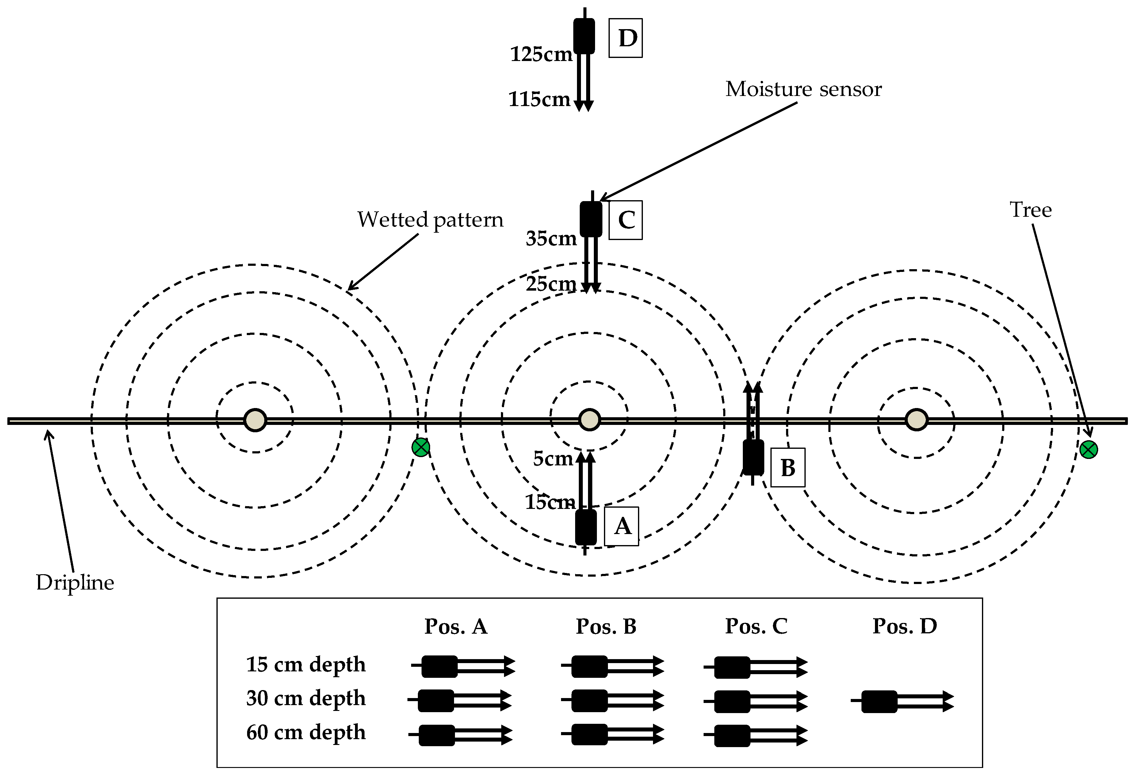
| A: center of wet bulb | 5–15 | 15, 30 and 60 |
| B: mid-point between two drippers | 25–35 | 15, 30 and 60 |
| C: wet area perimeter | 25–35 | 15, 30 and 60 |
| D: outside the influence of the dripper | 115–125 | 30 |
| Position | Depth (cm) | N | R2_Adj | Coef_SWC7 | Coef_bal | Coef_bal7 | |||
|---|---|---|---|---|---|---|---|---|---|
| A | 15 | 514 | 0.994 | 1.0021 | *** | 0.0036 | *** | 0.0007 | n.s |
| A | 30 | 514 | 0.998 | 0.9968 | *** | 0.0025 | *** | 0.0000 | n.s |
| A | 60 | 514 | 0.999 | 0.9971 | *** | 0.0009 | ** | 0.0003 | n.s |
| B | 15 | 514 | 0.997 | 0.9876 | *** | 0.0016 | *** | 0.0021 | *** |
| B | 30 | 514 | 0.982 | 0.9630 | *** | 0.0039 | *** | 0.0034 | *** |
| B | 60 | 514 | 1.000 | 0.9973 | *** | 0.0004 | * | 0.0013 | *** |
| C | 15 | 514 | 0.998 | 0.9808 | *** | −0.0002 | n.s | 0.0034 | *** |
| C | 30 | 514 | 0.998 | 0.9892 | *** | 0.0018 | *** | 0.0014 | *** |
| C | 60 | 514 | 0.999 | 0.9963 | *** | 0.0013 | *** | 0.0009 | ** |
| D | 30 | 260 | 1.000 | 0.9927 | *** | −0.0005 | ** | 0.0013 | *** |
| Position | Depth (cm) | N | R2_Adj | Coef_SWC7 | Coef_bal | Coef_bal7 | |||
|---|---|---|---|---|---|---|---|---|---|
| A | 15 | 514 | 0.999 | 0.9979 | *** | 0.0020 | *** | 0.0004 | n.s |
| A | 30 | 514 | 0.996 | 0.9963 | *** | 0.0032 | *** | 0.0006 | n.s |
| A | 60 | 514 | 0.997 | 0.9934 | *** | 0.0023 | *** | 0.0019 | *** |
| B | 15 | 514 | 0.999 | 0.9974 | *** | 0.0021 | *** | 0.0003 | n.s |
| B | 30 | 514 | 0.996 | 0.9951 | *** | 0.0031 | *** | 0.0007 | n.s |
| B | 60 | 514 | 0.997 | 0.9929 | *** | 0.0022 | *** | 0.0021 | *** |
| C | 15 | 514 | 0.999 | 0.9936 | *** | 0.0017 | *** | 0.0010 | *** |
| C | 30 | 514 | 0.997 | 0.9892 | *** | 0.0024 | *** | 0.0019 | *** |
| C | 60 | 514 | 0.998 | 0.9893 | *** | 0.0016 | *** | 0.0030 | *** |
| D | 30 | 260 | 0.999 | 0.9756 | *** | −0.0007 | *** | 0.0051 | *** |
© 2020 by the authors. Licensee MDPI, Basel, Switzerland. This article is an open access article distributed under the terms and conditions of the Creative Commons Attribution (CC BY) license (http://creativecommons.org/licenses/by/4.0/).
Share and Cite
Domínguez-Niño, J.M.; Oliver-Manera, J.; Arbat, G.; Girona, J.; Casadesús, J. Analysis of the Variability in Soil Moisture Measurements by Capacitance Sensors in a Drip-Irrigated Orchard. Sensors 2020, 20, 5100. https://doi.org/10.3390/s20185100
Domínguez-Niño JM, Oliver-Manera J, Arbat G, Girona J, Casadesús J. Analysis of the Variability in Soil Moisture Measurements by Capacitance Sensors in a Drip-Irrigated Orchard. Sensors. 2020; 20(18):5100. https://doi.org/10.3390/s20185100
Chicago/Turabian StyleDomínguez-Niño, Jesús María, Jordi Oliver-Manera, Gerard Arbat, Joan Girona, and Jaume Casadesús. 2020. "Analysis of the Variability in Soil Moisture Measurements by Capacitance Sensors in a Drip-Irrigated Orchard" Sensors 20, no. 18: 5100. https://doi.org/10.3390/s20185100