EEG-Based BCI Emotion Recognition: A Survey


Abstract
:1. Introduction
1.1. EEG-Based BCI in Emotion Recognition
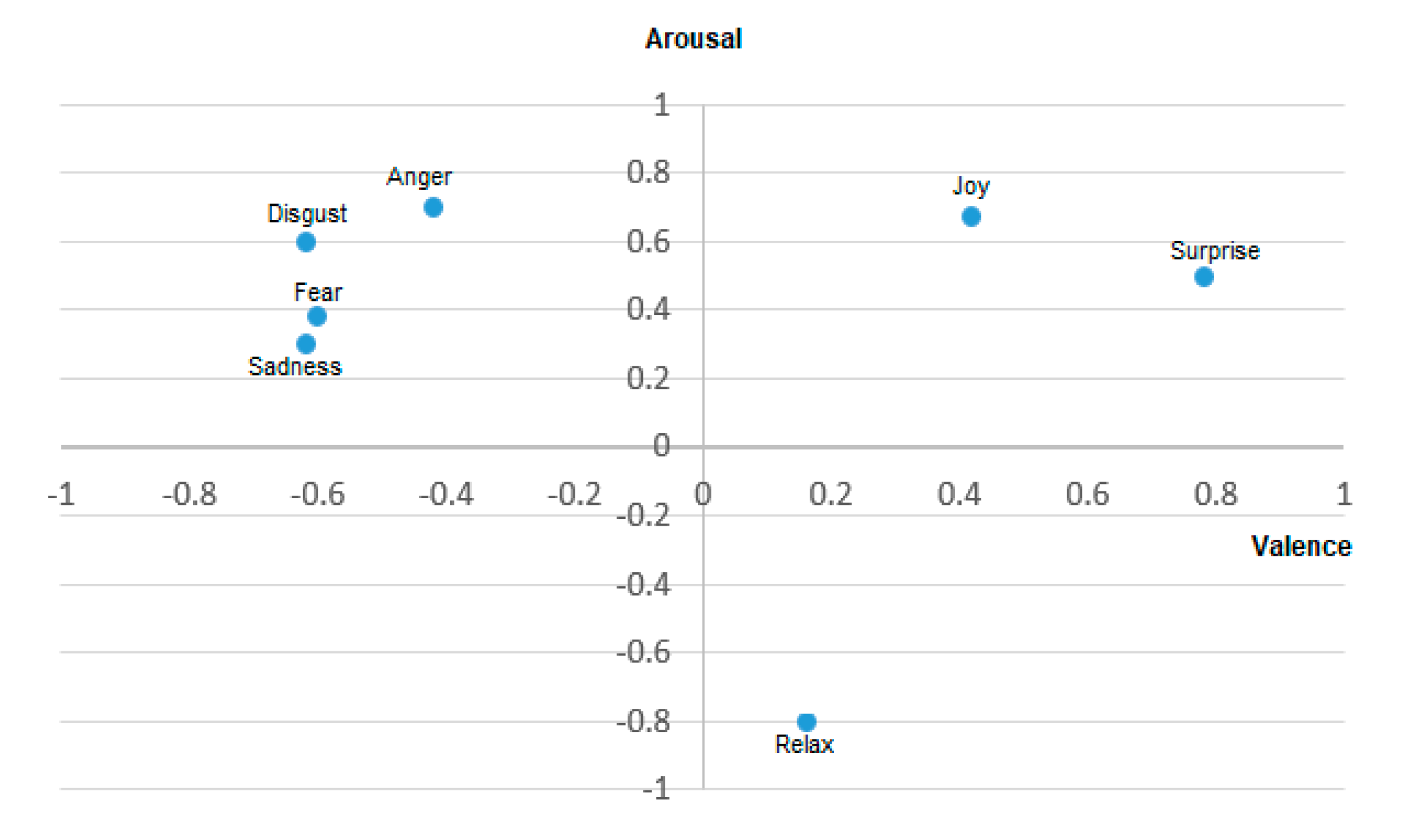
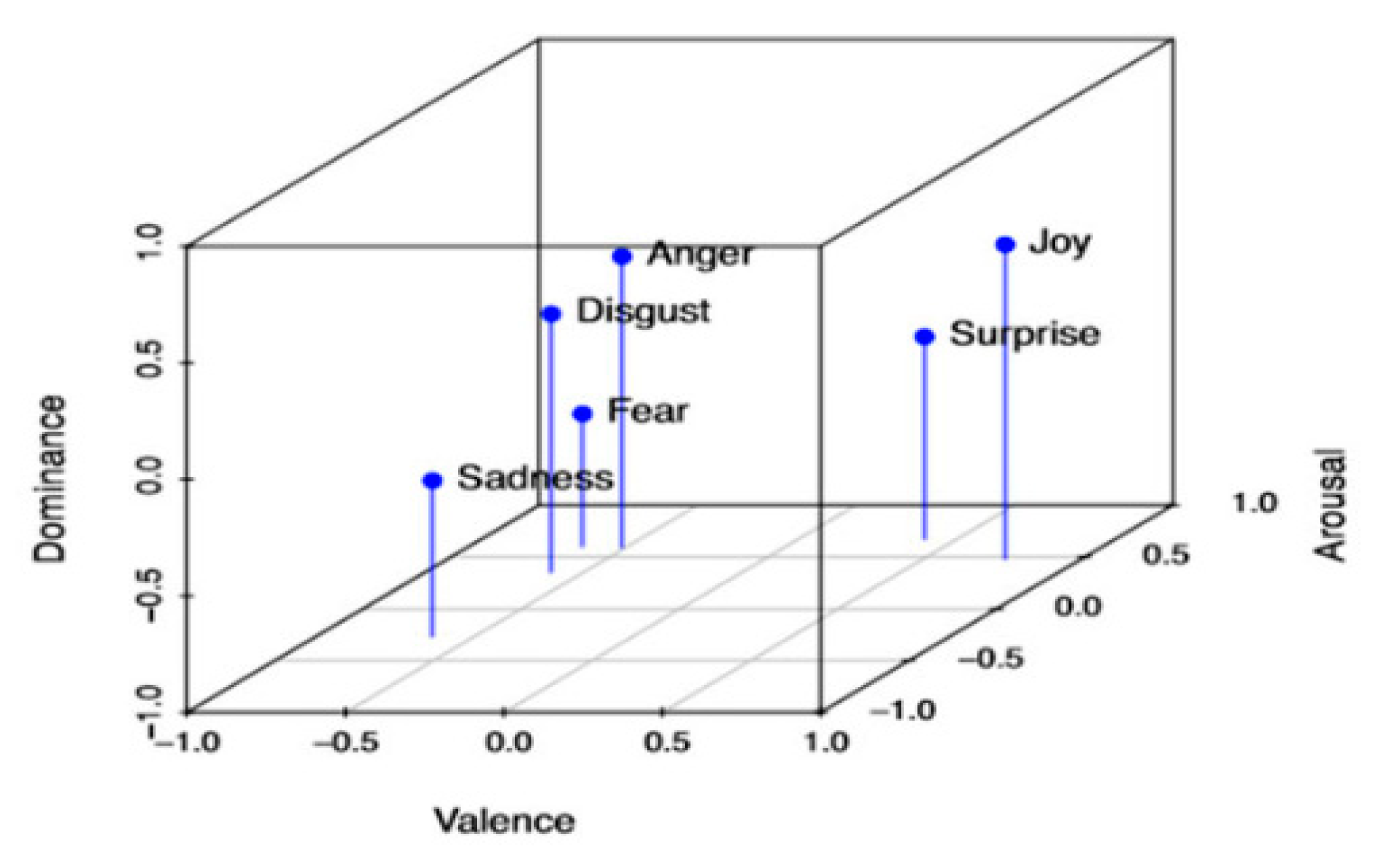
1.2. Emotion Representations
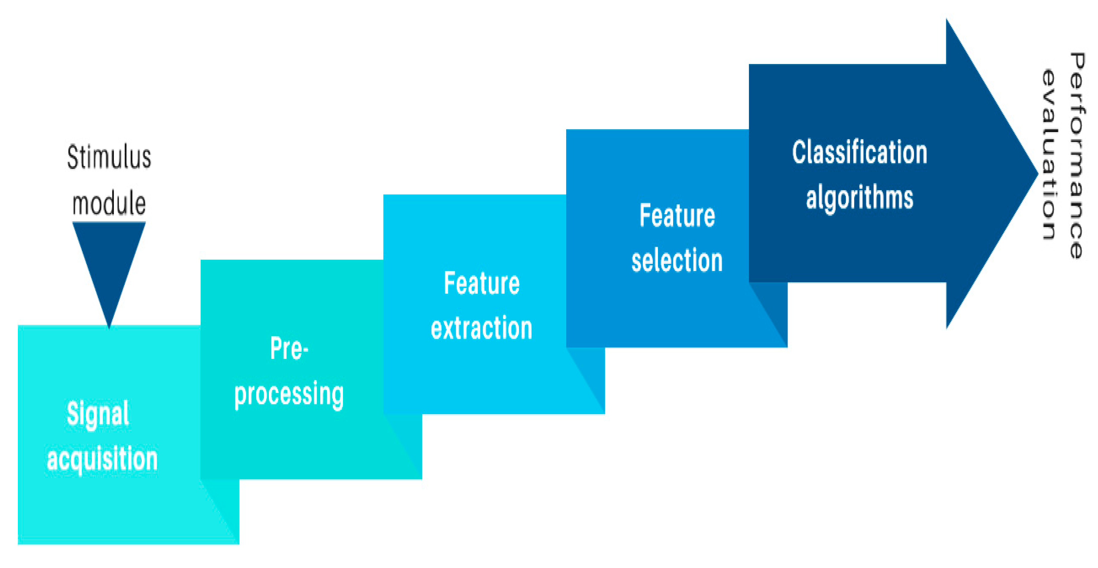
2. EEG-Based BCI Systems for Emotion Recognition
2.1. Signal Acquisition
2.1.1. Public Databases
2.1.2. Emotion Elicitation
2.1.3. Normalization
2.2. Preprocessing
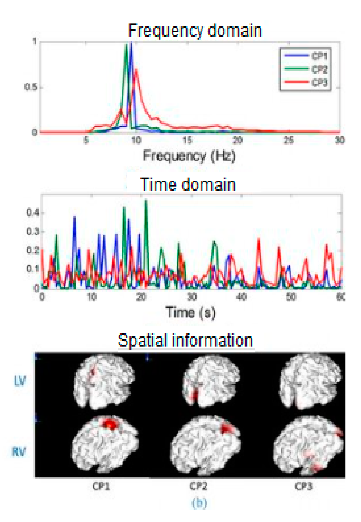
2.3. Feature Extraction
2.4. Feature Selection
- Filter methods evaluate features using the data’s intrinsic properties. Additionally, most of the filtering methods are univariate, so each feature is self-evaluated. These methods are appropriate for large data sets because they are less computationally expensive.
- Wrapping methods depend on classifier types when selecting new features based on their impact on characteristics already chosen. Only features that increase accuracy are selected.
- Built-in methods run internally in the classifier algorithms, such as deep learning. This type of process requires less computation than wrapper methods.
Examples of Feature Selection Algorithms
- Effect-size (ES)-based feature selection is a filter method.ES-based univariate: Cohen’s is an appropriate effect size for comparisons between two means [100]. So, if two groups’ means do not differ by 0.2 standard deviations or more, the difference is trivial, even if it is statistically significant. The effect size is calculated by taking the difference between the two groups and dividing it by the standard deviation of one of the groups. Univariate methods may discard features that could have provided useful information.ES-based multivariate helps remove several features with redundant information, therefore selecting fewer features, while retaining the most information [58]. It considers all the dependencies between characteristics when evaluating them. For example, calculating the Mahalanobis distance using the covariance structure of the noise.Min-redundancy max-relevance (mRMR) is a wrapper method [101]. This algorithm compares the mutual information between each feature with each class at the output. Mutual information between two random variables x and y is calculated as:where p (x) and p (y) are the marginal probability density functions of x and y, respectively, and p (x, y) is their joint probability function. If I (x, y) equals zero, the two random variables x and y are statistically independent [58].mRMR maximizes I (xi, y) between each characteristic xi and the target vector y; and minimizes the average mutual information I (xi, yi) between two characteristics.
- Stepwise discriminant analysis SDA [74]. SDA is the extension of the statistical tool for discriminant analysis that includes the stepwise technique.
- Fisher score is a feature selection technique to calculate interrelation between output classes and each feature using statistic measures [101].
2.5. Classification Algorithms
2.5.1. Generative Discriminative
2.5.2. Static-Dynamic Classification
2.5.3. Stable Unstable
2.5.4. Regularized
2.5.5. General Taxonomy of Classification Algorithms
2.6. Performance Evaluation
3. Literature Review of BCI Systems that Estimate Emotional States
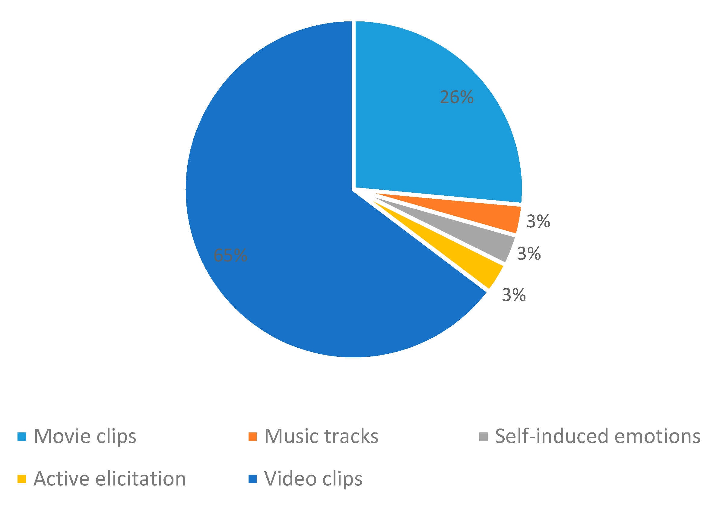
3.1. Emotion Elicitation Methods
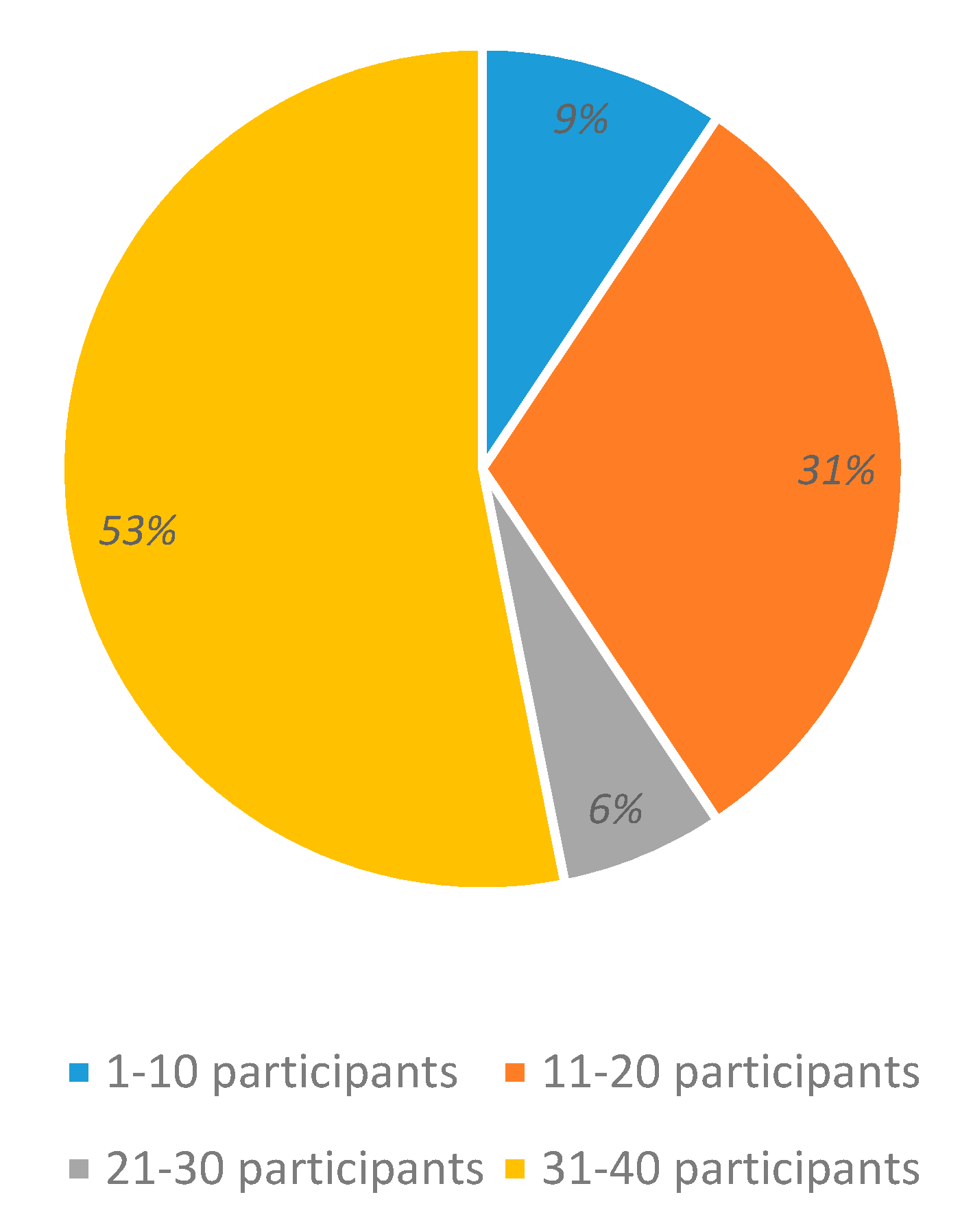
3.2. Number of Participants to Generate the System Dataset
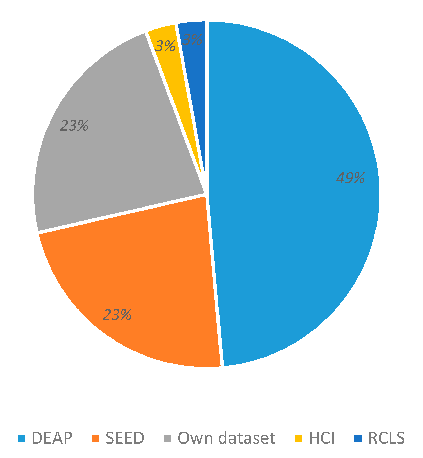
3.3. Datasets
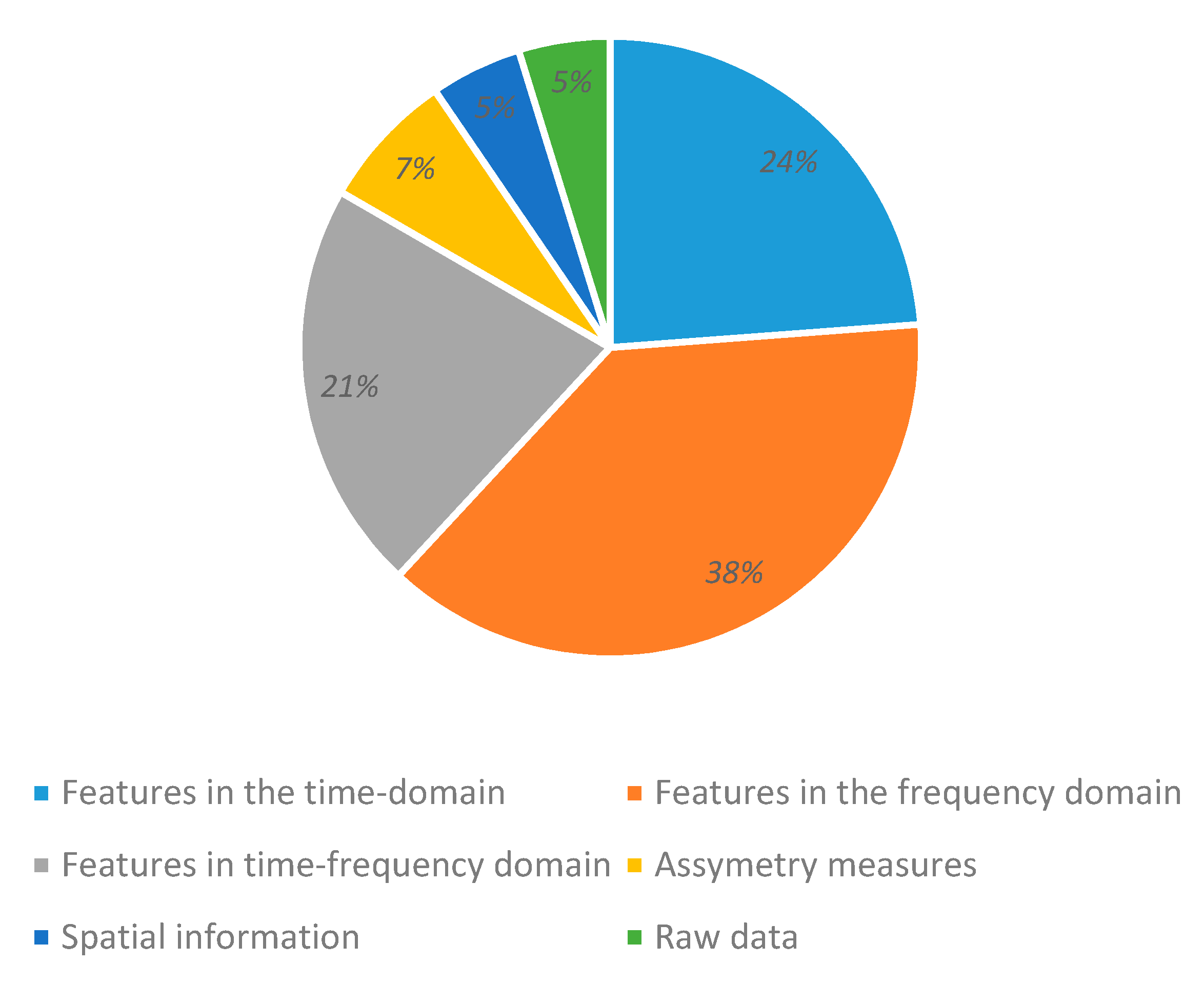
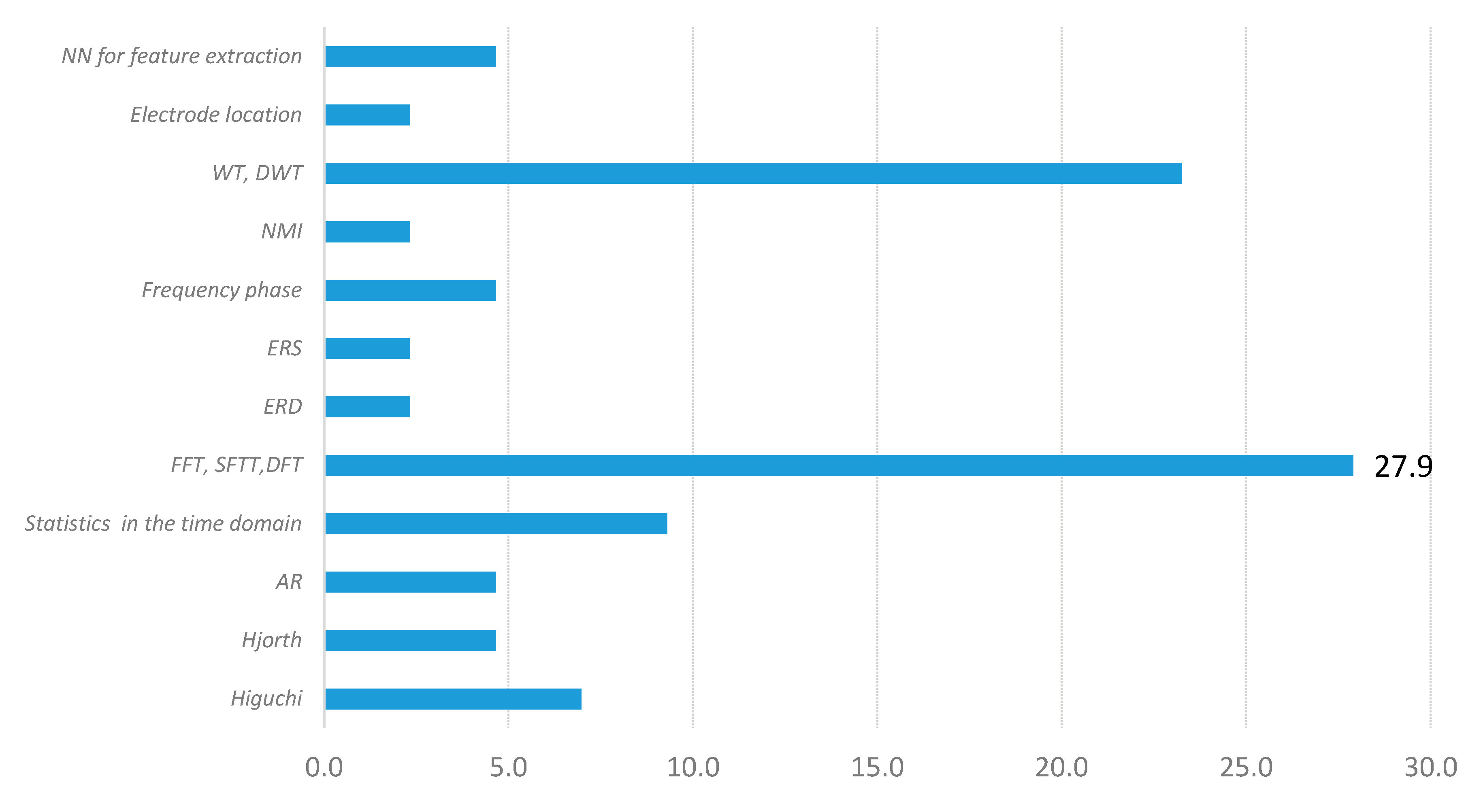
3.4. Feature Extraction
3.5. Feature Selection
3.6. Classifiers
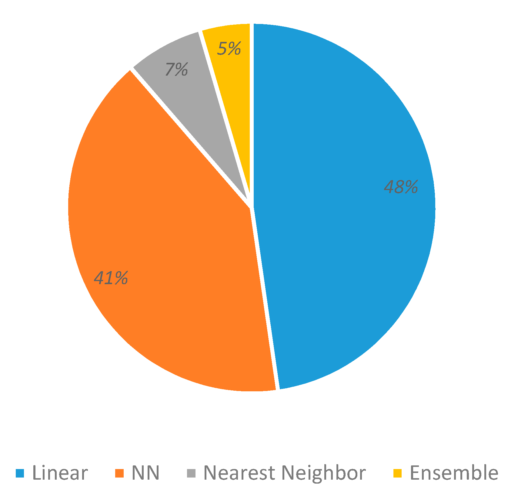
- Linear classifiers, such as naïve Bayes (NB), logistic regression (LR), support vector machine (SVM), linear discriminant analysis (LDA) (48% of use); and
- Neural networks like multi-layer perceptron (MLP), radial basis function RBF, convolutional neural network (CNN), deep belief networks (DBN), extreme learning method (ELM), graph regularized extreme learning machine (GELM), long short term memory (LSTM), domain adversarial neural network (DANN), Caps Net, and graph regularized sparse linear regularized (GRSLR) (41% of use).
- Ensemble classifiers like random forest, CART, bagging tree, Adaboost, and XGBoost are less used (5%). The same situation occurs with the kNN algorithm despite their consistently good performance results, probably because it works better with a simpler feature vector (7%).
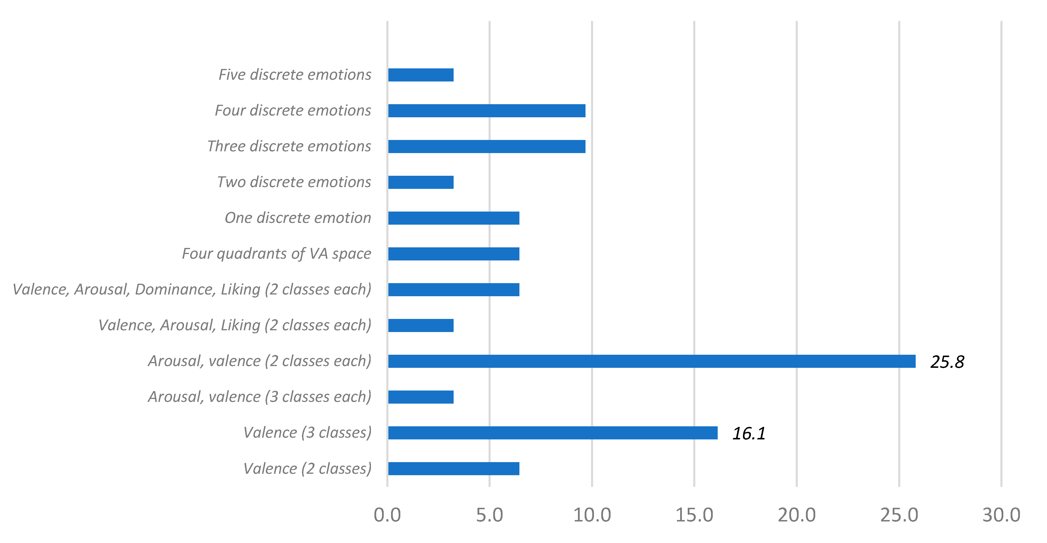
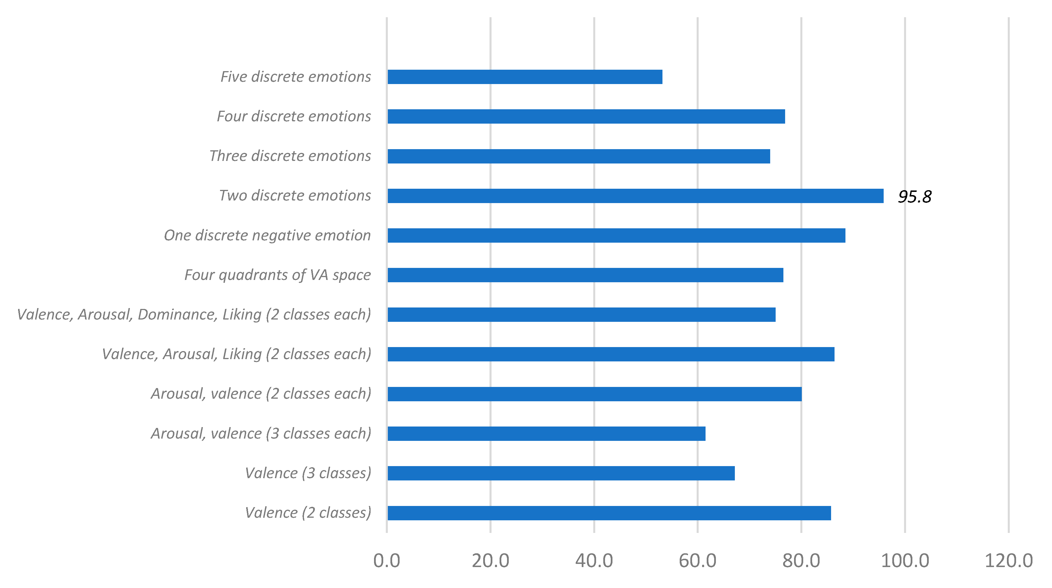
3.7. Performance vs. the Number of Classes-Emotions
4. Future Work
5. Conclusions
Author Contributions
Funding
Conflicts of Interest
References
- Picard, R.W. Affective Computing for HCI. In Proceedings of the HCI International 1999-Proceedings of the 8th International Conference on Human-Computer Interaction, Munich, Germany, 22–26 August 1999. [Google Scholar]
- Elfenbein, H.A.; Ambady, N. Predicting workplace outcomes from the ability to eavesdrop on feelings. J. Appl. Psychol. 2002, 87, 963–971. [Google Scholar] [CrossRef] [PubMed] [Green Version]
- Goenaga, S.; Navarro, L.; Quintero, C.G.M.; Pardo, M. Imitating human emotions with a nao robot as interviewer playing the role of vocational tutor. Electronics 2020, 9, 971. [Google Scholar] [CrossRef]
- Kitcheman, B. Procedures for performing systematic reviews. Comput. Sci. 2004, 1–28. Available online: http://www.inf.ufsc.br/~aldo.vw/kitchenham.pdf (accessed on 26 May 2020).
- Salzman, C.D.; Fusi, S. Emotion, cognition, and mental state representation in Amygdala and prefrontal Cortex. Annu. Rev. Neurosci. 2010, 33, 173–202. [Google Scholar] [CrossRef] [Green Version]
- Konar, A.; Chakraborty, A. Emotion Recognition: A Pattern Analysis Approach; John Wiley & Sons: Hoboken, NJ, USA, 2015; ISBN 9781118910566. [Google Scholar]
- Panoulas, K.J.; Hadjileontiadis, L.J.; Panas, S.M. Brain-Computer Interface (BCI): Types, Processing Perspectives and Applications; Springer: Berlin/Heidelberg, Germany, 2010; pp. 299–321. [Google Scholar]
- Ekman, P. Ekman 1992.pdf. Psychol. Rev. 1992, 99, 550–553. [Google Scholar] [CrossRef] [PubMed]
- Verma, G.K.; Tiwary, U.S. Affect representation and recognition in 3D continuous valence–arousal–dominance space. Multimed. Tools Appl. 2017, 76, 2159–2183. [Google Scholar] [CrossRef]
- Bălan, O.; Moise, G.; Moldoveanu, A.; Leordeanu, M.; Moldoveanu, F. Fear level classification based on emotional dimensions and machine learning techniques. Sensors 2019, 19, 1738. [Google Scholar] [CrossRef] [PubMed] [Green Version]
- Russell, J.A. A circumplex model of affect. J. Pers. Soc. Psychol. 1980, 39, 1161. [Google Scholar] [CrossRef]
- Bradley, M.M.; Lang, P.J. Measuring emotion: The self-assessment manikin and the semantic differential. J. Behav. Ther. Exp. Psychiatry 1994, 25, 49–59. [Google Scholar] [CrossRef]
- Ekman, P.; Davidson, R.J. Voluntary smiling changes regional brain activity. Psychol. Sci. 1993, 4, 342–345. [Google Scholar] [CrossRef]
- Bhatti, A.M.; Majid, M.; Anwar, S.M.; Khan, B. Human emotion recognition and analysis in response to audio music using brain signals. Comput. Human Behav. 2016, 65, 267–275. [Google Scholar] [CrossRef]
- Lee, Y.Y.; Hsieh, S. Classifying different emotional states by means of eegbased functional connectivity patterns. PLoS ONE 2014, 9, e95415. [Google Scholar] [CrossRef]
- Zheng, W.L.; Guo, H.T.; Lu, B.L. Revealing critical channels and frequency bands for emotion recognition from EEG with deep belief network. Int. IEEE/EMBS Conf. Neural Eng. NER 2015, 2015, 154–157. [Google Scholar] [CrossRef]
- Knyazev, G.G.; Slobodskoj-Plusnin, J.Y. Behavioural approach system as a moderator of emotional arousal elicited by reward and punishment cues. Pers. Individ. Dif. 2007, 42, 49–59. [Google Scholar] [CrossRef]
- Kirmizi-Alsan, E.; Bayraktaroglu, Z.; Gurvit, H.; Keskin, Y.H.; Emre, M.; Demiralp, T. Comparative analysis of event-related potentials during Go/NoGo and CPT: Decomposition of electrophysiological markers of response inhibition and sustained attention. Brain Res. 2006, 1104, 114–128. [Google Scholar] [CrossRef]
- Hyvarinen, A. New Approximations of differential entropy for independent component analysis and projection pursuit. In Proceedings of the Advances in Neural Information Processing Systems, Denver, CO, USA; 1998; pp. 273–279. [Google Scholar]
- Hamann, S. Mapping discrete and dimensional emotions onto the brain: Controversies and consensus. Trends Cogn. Sci. 2012, 16, 458–466. [Google Scholar] [CrossRef]
- Davidson, R.J.; Ekman, P.; Saron, C.D.; Senulis, J.A.; Friesen, W.V. Approach-withdrawl-and-cerebral-asymmetry-emotional-expres davidson 1990.pdf. J. Pers. Soc. Psychol. 1990, 58, 330–341. [Google Scholar] [CrossRef]
- Peterson, V.; Galván, C.; Hernández, H.; Spies, R. A feasibility study of a complete low-cost consumer-grade brain-computer interface system. Heliyon 2020, 6. [Google Scholar] [CrossRef]
- Savran, A.; Ciftci, K.; Chanel, G.; Mota, J.C.; Viet, L.H.; Sankur, B.; Akarun, L.; Caplier, A.; Rombaut, M. Emotion detection in the loop from brain signals and facial images. eNTERFACE 2006, 6, 69–80. [Google Scholar]
- Onton, J.; Makeig, S. High-frequency broadband modulations of electroencephalographic spectra. Front. Hum. Neurosci. 2009, 3, 1–18. [Google Scholar] [CrossRef] [Green Version]
- Yadava, M.; Kumar, P.; Saini, R.; Roy, P.P.; Prosad Dogra, D. Analysis of EEG signals and its application to neuromarketing. Multimed. Tools Appl. 2017, 76, 19087–19111. [Google Scholar] [CrossRef]
- Zheng, W.L.; Liu, W.; Lu, Y.; Lu, B.L.; Cichocki, A. EmotionMeter: A Multimodal framework for recognizing human emotions. IEEE Trans. Cybern. 2019, 49, 1110–1122. [Google Scholar] [CrossRef] [PubMed]
- Soleymani, M.; Lichtenauer, J.; Pun, T.; Pantic, M. A multimodal database for affect recognition and implicit tagging. IEEE Trans. Affect. Comput. 2012, 3, 42–55. [Google Scholar] [CrossRef] [Green Version]
- Grégoire, C.; Rodrigues, P.L.C.; Congedo, M. EEG Alpha Waves Dataset; Centre pour la Communication Scientifique Directe: Grenoble, France, 2019. [Google Scholar]
- Katsigiannis, S.; Ramzan, N. DREAMER: A database for emotion recognition through EEG and ECG signals from wireless low-cost off-the-shelf devices. IEEE J. Biomed. Heal. Informatics 2018, 22, 98–107. [Google Scholar] [CrossRef] [Green Version]
- Li, Y.; Zheng, W.; Cui, Z.; Zong, Y.; Ge, S. EEG emotion recognition based on graph regularized sparse linear regression. Neural Process. Lett. 2019, 49, 555–571. [Google Scholar] [CrossRef]
- Lang, P.J.; Bradley, M.M.; Cuthbert, B.N. International affective picture system (IAPS): Technical manual and affective ratings. NIMH Cent. Study Emot. Atten. 1997, 1, 39–58. [Google Scholar]
- Yang, W.; Makita, K.; Nakao, T.; Kanayama, N.; Machizawa, M.G.; Sasaoka, T.; Sugata, A.; Kobayashi, R.; Hiramoto, R.; Yamawaki, S.; et al. Affective auditory stimulus database: An expanded version of the International Affective Digitized Sounds (IADS-E). Behav. Res. Methods 2018, 50, 1415–1429. [Google Scholar] [CrossRef]
- Mühl, C.; Allison, B.; Nijholt, A.; Chanel, G. A survey of affective brain computer interfaces: Principles, state-of-the-art, and challenges. Brain Comput. Interfaces 2014, 1, 66–84. [Google Scholar] [CrossRef] [Green Version]
- Zhou, F.; Qu, X.; Jiao, J.; Helander, M.G. Emotion prediction from physiological signals: A comparison study between visual and auditory elicitors. Interact. Comput. 2014, 26, 285–302. [Google Scholar] [CrossRef]
- Pallavicini, F.; Ferrari, A.; Pepe, A.; Garcea, G. Effectiveness of virtual reality survival horror games for the emotional elicitation: Preliminary insights using Resident Evil 7: Biohazard. In International Conference on Universal Access in Human-Computer Interaction; Springer: Cham, Switzerland, 2018. [Google Scholar] [CrossRef]
- Roza, V.C.C.; Postolache, O.A. Multimodal approach for emotion recognition based on simulated flight experiments. Sensors 2019, 19, 5516. [Google Scholar] [CrossRef] [PubMed] [Green Version]
- Iacoviello, D.; Petracca, A.; Spezialetti, M.; Placidi, G. A real-time classification algorithm for EEG-based BCI driven by self-induced emotions. Comput. Methods Programs Biomed. 2015, 122, 293–303. [Google Scholar] [CrossRef] [PubMed] [Green Version]
- Novak, D.; Mihelj, M.; Munih, M. A survey of methods for data fusion and system adaptation using autonomic nervous system responses in physiological computing. Interact. Comput. 2012, 24, 154–172. [Google Scholar] [CrossRef]
- Bustamante, P.A.; Lopez Celani, N.M.; Perez, M.E.; Quintero Montoya, O.L. Recognition and regionalization of emotions in the arousal-valence plane. In Proceedings of the 2015 Milano, Italy 37th Annual International Conference of the IEEE Engineering in Medicine and Biology Society (EMBC), Milano, Italy, 25–29 August 2015; Volume 2015, pp. 6042–6045. [Google Scholar]
- Sanei, S.; Chambers, J.A. EEG Signal Processing; John Wiley & Sons: Hoboken, NJ, USA, 2013; ISBN 9780470025819. [Google Scholar]
- Abhang, P.A.; Suresh, C.; Mehrotra, B.W.G. Introduction to EEG-and Speech-Based Emotion Recognition; Elsevier: Amsterdam, The Netherlands, 2016; ISBN 9780128044902. [Google Scholar]
- Jardim-Gonçalves, R.; Universidade Nova de Lisboa. Faculdade de Ciências e Tecnologia; Institute of Electrical and Electronics Engineers; IEEE Technology Engineering and Management Society. In Proceedings of the IEEE International Technology Management Conference, Madeira Islands, Portugal, 27–29 June 2017; International Conference on Engineering, Technology and Innovation (ICE/ITMC) : “Engineering, technology & innovation management beyond 2020: New challenges, new approaches” : Conference proceedings. ISBN 9781538607749. [Google Scholar]
- Alhaddad, M.J.; Kamel, M.; Malibary, H.; Thabit, K.; Dahlwi, F.; Hadi, A. P300 speller efficiency with common average reference. Lect. Notes Comput. Sci. 2012, 7326 LNAI, 234–241. [Google Scholar] [CrossRef]
- Alhaddad, M.J.; Kamel, M.; Malibary, H.; Thabit, K.; Dahlwi, F.; Hadi, A. P300 speller efficiency with common average reference. In Proceedings of the International Conference on Autonomous and Intelligent Systems, Aveiro, Portugal, 25–27 June 2012; pp. 234–241. [Google Scholar]
- Murugappan, M.; Nagarajan, R.; Yaacob, S. Combining spatial filtering and wavelet transform for classifying human emotions using EEG Signals. J. Med. Biol. Eng. 2011, 31, 45–51. [Google Scholar] [CrossRef]
- Murugappan, M.; Murugappan, S. Human emotion recognition through short time Electroencephalogram (EEG) signals using Fast Fourier Transform (FFT). In Proceedings of the Proceedings-2013 IEEE 9th International Colloquium on Signal Processing and its Applications, Kuala Lumpur, Malaysia, 8–10 March 2013; pp. 289–294. [Google Scholar]
- Burle, B.; Spieser, L.; Roger, C.; Casini, L.; Hasbroucq, T.; Vidal, F. Spatial and temporal resolutions of EEG: Is it really black and white? A scalp current density view. Int. J. Psychophysiol. 2015, 97, 210–220. [Google Scholar] [CrossRef]
- Mazumder, I. An analytical approach of EEG analysis for emotion recognition. In Proceedings of the 2019 Devices for Integrated Circuit (DevIC), Kalyani, India, 23 March 2019; pp. 256–260. [Google Scholar] [CrossRef]
- Subasi, A.; Gursoy, M.I. EEG signal classification using PCA, ICA, LDA and support vector machines. Expert Syst. Appl. 2010, 37, 8659–8666. [Google Scholar] [CrossRef]
- Lee, H.; Choi, S. Pca + hmm + svm for eeg pattern classification. In Proceedings of the Seventh International Symposium on Signal Processing and Its Applications, Paris, France, 4 July 2003; pp. 541–544. [Google Scholar]
- Doma, V.; Pirouz, M. A comparative analysis of machine learning methods for emotion recognition using EEG and peripheral physiological signals. J. Big Data 2020, 7. [Google Scholar] [CrossRef] [Green Version]
- Shaw, L.; Routray, A. Statistical features extraction for multivariate pattern analysis in meditation EEG using PCA. In Proceedings of the 2016 IEEE EMBS International Student Conference ISC, Ottawa, ON, Canada, 31 May 2016; pp. 1–4. [Google Scholar] [CrossRef]
- Symposium, I.; Analysis, I.C.; Separation, B.S. 4th International Symposium on Independent Component Analysis and Blind Signal Separation (ICA2003), April 2003, Nara, Japan. Analysis 2003, 975–980. [Google Scholar]
- Liu, J.; Meng, H.; Li, M.; Zhang, F.; Qin, R.; Nandi, A.K. Emotion detection from EEG recordings based on supervised and unsupervised dimension reduction. Concurr. Comput. 2018, 30, 1–13. [Google Scholar] [CrossRef] [Green Version]
- Yong, X.; Ward, R.K.; Birch, G.E. Robust common spatial patterns for EEG signal preprocessing. In Proceedings of the 30th Annual International Conference of the IEEE Engineering in Medicine and Biology Society, EMBS’08-“Personalized Healthcare through Technology”, Boston, MA, USA, 30 August 2011; pp. 2087–2090. [Google Scholar]
- Li, X.; Fan, H.; Wang, H.; Wang, L. Common spatial patterns combined with phase synchronization information for classification of EEG signals. Biomed. Signal Process. Control 2019, 52, 248–256. [Google Scholar] [CrossRef]
- Interfaces, B. A Tutorial on EEG signal processing techniques for mental state recognition in brain-computer interfaces. Guid. Brain Comput. Music Interfacing 2014. [Google Scholar] [CrossRef]
- Jenke, R.; Peer, A.; Buss, M. Feature extraction and selection for emotion recognition from EEG. IEEE Trans. Affect. Comput. 2014, 5, 327–339. [Google Scholar] [CrossRef]
- Al-Fahoum, A.S.; Al-Fraihat, A.A. Methods of EEG signal features extraction using linear analysis in frequency and time-frequency domains. ISRN Neurosci. 2014, 2014, 1–7. [Google Scholar] [CrossRef] [PubMed] [Green Version]
- Petrantonakis, P.C.; Hadjileontiadis, L.J. Emotion recognition from brain signals using hybrid adaptive filtering and higher order crossings analysis. IEEE Trans. Affect. Comput. 2010, 1, 81–97. [Google Scholar] [CrossRef]
- Torres, E.P.; Torres, E.A.; Hernandez-Alvarez, M.; Yoo, S.G. Machine learning analysis of EEG measurements of stock trading performance. In Advances in Artificial Intelligence, Software and Systems Engineering; Springer Nature: Lodon, UK, 2020. [Google Scholar]
- Kubben, P.; Dumontier, M.; Dekker, A. Fundamentals of clinical data science. Fundam. Clin. Data Sci. 2018, 1–219. [Google Scholar] [CrossRef] [Green Version]
- Karahan, E.; Rojas-Lopez, P.A.; Bringas-Vega, M.L.; Valdes-Hernandez, P.A.; Valdes-Sosa, P.A. Tensor analysis and fusion of multimodal brain images. Proc. IEEE 2015, 103, 1531–1559. [Google Scholar] [CrossRef]
- Winkler, I.; Debener, S.; Muller, K.R.; Tangermann, M. On the influence of high-pass filtering on ICA-based artifact reduction in EEG-ERP. In Proceedings of the 2015 37th Annual International Conference of the IEEE Engineering in Medicine and Biology Society (EMBC), Milan, Italy, 25–29 August 2015. [Google Scholar] [CrossRef]
- Zhang, Y.; Zhou, G.; Zhao, Q.; Jin, J.; Wang, X.; Cichocki, A. Spatial-temporal discriminant analysis for ERP-based brain-computer interface. IEEE Trans. Neural Syst. Rehabil. Eng. 2013, 21, 233–243. [Google Scholar] [CrossRef]
- Brouwer, A.M.; Zander, T.O.; Van Erp, J.B.F.; Korteling, J.E.; Bronkhorst, A.W. Using neurophysiological signals that reflect cognitive or affective state: Six recommendations to avoid common pitfalls. Front. Neurosci. 2015, 9, 1–11. [Google Scholar] [CrossRef] [Green Version]
- Wu, Z.; Yao, D.; Tang, Y.; Huang, Y.; Su, S. Amplitude modulation of steady-state visual evoked potentials by event-related potentials in a working memory task. J. Biol. Phys. 2010, 36, 261–271. [Google Scholar] [CrossRef] [Green Version]
- Abootalebi, V.; Moradi, M.H.; Khalilzadeh, M.A. A new approach for EEG feature extraction in P300-based lie detection. Comput. Methods Programs Biomed. 2009, 94, 48–57. [Google Scholar] [CrossRef] [PubMed]
- Bhise, P.R.; Kulkarni, S.B.; Aldhaheri, T.A. Brain computer interface based EEG for emotion recognition system: A systematic review. In Proceedings of the 2020 2nd International Conference on Innovative Mechanisms for Industry Applications (ICIMIA), Bangalore, India, 5–7 March 2020; ISBN 9781728141671. [Google Scholar]
- Li, X.; Song, D.; Zhang, P.; Zhang, Y.; Hou, Y.; Hu, B. Exploring EEG features in cross-subject emotion recognition. Front. Neurosci. 2018, 12. [Google Scholar] [CrossRef] [PubMed] [Green Version]
- Liu, Y.; Sourina, O. EEG databases for emotion recognition. In Proceedings of the 2013 International Conference on Cyberworlds, Yokohama, Japan, 21–23 October 2013; pp. 302–309. [Google Scholar]
- Hossain, M.Z.; Kabir, M.M.; Shahjahan, M. Feature selection of EEG data with neuro-statistical method. In Proceedings of the 2013 International Conference on Electrical Information and Communication Technology (EICT), Khulna, Bangladesh, 13–15 February 2014. [Google Scholar] [CrossRef]
- Bavkar, S.; Iyer, B.; Deosarkar, S. Detection of alcoholism: An EEG hybrid features and ensemble subspace K-NN based approach. In Proceedings of the International Conference on Distributed Computing and Internet Technology, Bhubaneswar, India, 10–13 January 2019; pp. 161–168. [Google Scholar]
- Pane, E.S.; Wibawa, A.D.; Pumomo, M.H. Channel Selection of EEG Emotion Recognition using Stepwise Discriminant Analysis. In Proceedings of the 2018 International Conference on Computer Engineering, Network and Intelligent Multimedia (CENIM), Surabaya, Indonesia, 26–27 November 2018; pp. 14–19. [Google Scholar] [CrossRef]
- Musselman, M.; Djurdjanovic, D. Time-frequency distributions in the classification of epilepsy from EEG signals. Expert Syst. Appl. 2012, 39, 11413–11422. [Google Scholar] [CrossRef]
- Xu, H.; Plataniotis, K.N. Affect recognition using EEG signal. In Proceedings of the 2012 IEEE 14th International Workshop on Multimedia Signal Processing (MMSP), Banff, AB, Canada, 17 September 2012; pp. 299–304. [Google Scholar] [CrossRef]
- Wu, X.; Zheng, W.-L.; Lu, B.-L. Investigating EEG-Based Functional Connectivity Patterns for Multimodal Emotion Recognition. 2020. Available online: https://arxiv.org/abs/2004.01973 (accessed on 26 May 2020).
- Zheng, W.-L.; Zhu, J.-Y.; Lu, B.-L. Identifying Stable Patterns over Time for Emotion Recognition from EEG. IEEE Trans. Affect. Comput. 2017, 10, 417–429. [Google Scholar] [CrossRef] [Green Version]
- Yang, Y.; Wu, Q.M.J.; Zheng, W.L.; Lu, B.L. EEG-based emotion recognition using hierarchical network with subnetwork nodes. IEEE Trans. Cogn. Dev. Syst. 2018, 10, 408–419. [Google Scholar] [CrossRef]
- Li, P.; Liu, H.; Si, Y.; Li, C.; Li, F.; Zhu, X.; Huang, X.; Zeng, Y.; Yao, D.; Zhang, Y.; et al. EEG based emotion recognition by combining functional connectivity network and local activations. IEEE Trans. Biomed. Eng. 2019, 66, 2869–2881. [Google Scholar] [CrossRef]
- Li, Z.; Tian, X.; Shu, L.; Xu, X.; Hu, B. Emotion recognition from EEG using RASM and LSTM. In Proceedings of the International Conference on Internet Multimedia Computing and Service, Qingdao, China, 23–25 August 2017; pp. 310–318. [Google Scholar]
- Mowla, M.R.; Cano, R.I.; Dhuyvetter, K.J.; Thompson, D.E. Affective brain-computer interfaces: A tutorial to choose performance measuring metric. arXiv 2020, arXiv:2005.02619. [Google Scholar]
- Lan, Z.; Sourina, O.; Wang, L.; Scherer, R.; Muller-Putz, G.R. Domain adaptation techniques for eeg-based emotion recognition: A comparative study on two public datasets. IEEE Trans. Cogn. Dev. Syst. 2019, 11, 85–94. [Google Scholar] [CrossRef]
- Duan, R.N.; Zhu, J.Y.; Lu, B.L. Differential entropy feature for EEG-based emotion classification. In Proceedings of the International IEEE/EMBS Conference on Neural Engineering, San Diego, CA, USA, 6–8 November 2013; pp. 81–84. [Google Scholar]
- Zheng, W.L.; Lu, B.L. Investigating critical frequency bands and channels for eeg-based emotion recognition with deep neural networks. IEEE Trans. Auton. Ment. Dev. 2015, 7, 162–175. [Google Scholar] [CrossRef]
- Assistant Professor, T.S.; Ravi Kumar Principal, K.M.; Nataraj, A.; K Students, A.K. Analysis of EEG Based Emotion Detection of DEAP and SEED-IV Databases Using SVM. Available online: https://papers.ssrn.com/sol3/papers.cfm?abstract_id=3509130 (accessed on 26 May 2020).
- Wang, X.H.; Zhang, T.; Xu, X.M.; Chen, L.; Xing, X.F.; Chen, C.L.P. EEG Emotion Recognition Using Dynamical Graph Convolutional Neural Networks and Broad Learning System. In Proceedings of the 2018 IEEE International Conference on Bioinformatics and Biomedicine (BIBM), Madrid, Spain, 3–6 December 2018; pp. 1240–1244. [Google Scholar] [CrossRef]
- Li, J.; Qiu, S.; Du, C.; Wang, Y.; He, H. Domain adaptation for eeg emotion recognition based on latent representation similarity. IEEE Trans. Cogn. Dev. Syst. 2020, 12, 344–353. [Google Scholar] [CrossRef]
- Petrantonakis, P.C.; Hadjileontiadis, L.J. Emotion recognition from EEG using higher order crossings. IEEE Trans. Inf. Technol. Biomed. 2010, 14, 186–197. [Google Scholar] [CrossRef] [PubMed]
- Kim, M.K.; Kim, M.; Oh, E.; Kim, S.P. A review on the computational methods for emotional state estimation from the human EEG. Comput. Math. Methods Med. 2013, 2013. [Google Scholar] [CrossRef] [PubMed] [Green Version]
- Yoon, H.J.; Chung, S.Y. EEG-based emotion estimation using Bayesian weighted-log-posterior function and perceptron convergence algorithm. Comput. Biol. Med. 2013, 43, 2230–2237. [Google Scholar] [CrossRef] [PubMed]
- Hosni, S.M.; Gadallah, M.E.; Bahgat, S.F.; AbdelWahab, M.S. Classification of EEG signals using different feature extraction techniques for mental-task BCI. In Proceedings of the ICCES’07-2007 International Conference on Computer Engineering and Systems, Cairo, Egypt, 27–29 November 2007; pp. 220–226. [Google Scholar]
- Xing, X.; Li, Z.; Xu, T.; Shu, L.; Hu, B.; Xu, X. SAE+LSTM: A new framework for emotion recognition from multi-channel EEG. Front. Neurorobot. 2019, 13, 1–14. [Google Scholar] [CrossRef] [PubMed]
- Navarro, I.; Sepulveda, F.; Hubais, B. A comparison of time, frequency and ICA based features and five classifiers for wrist movement classification in EEG signals. Conf. Proc. IEEE Eng. Med. Biol. Soc. 2005, 2005, 2118–2121. [Google Scholar]
- Ting, W.; Guo-zheng, Y.; Bang-hua, Y.; Hong, S. EEG feature extraction based on wavelet packet decomposition for brain computer interface. Meas. J. Int. Meas. Confed. 2008, 41, 618–625. [Google Scholar] [CrossRef]
- Guo, J.; Fang, F.; Wang, W.; Ren, F. EEG emotion recognition based on granger causality and capsnet neural network. In Proceedings of the 2018 5th IEEE International Conference on Cloud Computing and Intelligence Systems (CCIS), Nanjing, China, 23–25 November 2018; pp. 47–52. [Google Scholar] [CrossRef]
- Sander, D.; Grandjean, D.; Scherer, K.R. A systems approach to appraisal mechanisms in emotion. Neural Netw. 2005, 18, 317–352. [Google Scholar] [CrossRef]
- Chanel, G.; Kierkels, J.J.M.; Soleymani, M.; Pun, T. Short-term emotion assessment in a recall paradigm. Int. J. Hum. Comput. Stud. 2009, 67, 607–627. [Google Scholar] [CrossRef]
- Lotte, F.; Congedo, M.; Lécuyer, A.; Lamarche, F.; Arnaldi, B.; Anatole, L.; Lotte, F.; Congedo, M.; Anatole, L.; Abdulhay, E.; et al. A review of classification algorithms for EEG-based brain–Computer interfaces To cite this version: A review of classification algorithms for EEG-based brain-computer interfaces. Hum. Brain Mapp. 2018, 38, 270–278. [Google Scholar] [CrossRef] [Green Version]
- Jenke, R.; Peer, A.; Buss, M. Effect-size-based Electrode and Feature Selection for Emotion Recognition from EEG. In Proceedings of the 2013 IEEE International Conference on Acoustics, Speech and Signal Processing, Vancouver, Canada, 26–31 May 2013; pp. 1217–1221. [Google Scholar]
- Hassanien, A.E.; Azar, A.T. (Eds.) Intelligent Systems Reference Library 74 Brain-Computer Interfaces Current Trends and Applications; Springer: Berlin/Heidelberg, Germany, 2015. [Google Scholar]
- Zhang, L.; Xiong, G.; Liu, H.; Zou, H.; Guo, W. Time-frequency representation based on time-varying autoregressive model with applications to non-stationary rotor vibration analysis. Sadhana Acad. Proc. Eng. Sci. 2010, 35, 215–232. [Google Scholar] [CrossRef]
- Hill, N.J.; Wolpaw, J.R. Brain–Computer Interface. In Reference Module in Biomedical Sciences; Elsevier: Amsterdam, The Netherlands, 2016. [Google Scholar]
- Rashid, M.; Sulaiman, N.P.P.; Abdul Majeed, A.; Musa, R.M.; Ab. Nasir, A.F.; Bari, B.S.; Khatun, S. Current Status, Challenges, and Possible Solutions of EEG-Based Brain-Computer Interface: A Comprehensive Review. Front. Neurorobot. 2020, 14. [Google Scholar] [CrossRef] [PubMed]
- Vaid, S.; Singh, P.; Kaur, C. EEG signal analysis for BCI interface: A review. In Proceedings of the International Conference on Advanced Computing and Communication Technologies, Haryana, India, 21 February 2015; pp. 143–147. [Google Scholar]
- Ackermann, P.; Kohlschein, C.; Bitsch, J.Á.; Wehrle, K.; Jeschke, S. EEG-based automatic emotion recognition: Feature extraction, selection and classification methods. In Proceedings of the 2016 IEEE 18th international conference on e-health networking, applications and services (Healthcom), Munich, Germany, 14–16 September 2016. [Google Scholar] [CrossRef]
- Atangana, R.; Tchiotsop, D.; Kenne, G.; DjoufackNkengfac k, L.C. EEG signal classification using LDA and MLP classifier. Heal. Inform. An Int. J. 2020, 9, 14–32. [Google Scholar] [CrossRef]
- Srivastava, S.; Gupta, M.R.; Frigyik, B.A. Bayesian quadratic discriminant analysis. J. Mach. Learn. Res. 2007, 8, 1277–1305. [Google Scholar]
- Cimtay, Y.; Ekmekcioglu, E. Investigating the use of pretrained convolutional neural network on cross-subject and cross-dataset eeg emotion recognition. Sensors 2020, 20, 34. [Google Scholar] [CrossRef] [PubMed] [Green Version]
- Tzirakis, P.; Trigeorgis, G.; Nicolaou, M.A.; Schuller, B.W.; Zafeiriou, S. End-to-end multimodal emotion recognition using deep neural networks. IEEE J. Sel. Top. Signal Process. 2017, 11, 1301–1309. [Google Scholar] [CrossRef] [Green Version]
- Chen, J.X.; Zhang, P.W.; Mao, Z.J.; Huang, Y.F.; Jiang, D.M.; Zhang, Y.N. Accurate EEG-based emotion recognition on combined features using deep convolutional neural networks. IEEE Access 2019, 7, 44317–44328. [Google Scholar] [CrossRef]
- Zhang, W.; Wang, F.; Jiang, Y.; Xu, Z.; Wu, S.; Zhang, Y. Cross-Subject EEG-Based Emotion Recognition with Deep Domain Confusion; Springer International Publishing: Berlin/Heidelberg, Germany, 2019; ISBN 9783030275259. [Google Scholar]
- Lechner, U. Scientific Workflow Scheduling for Cloud Computing Environments; Springer International Publishing: Berlin/Heidelberg, Germany, 2019; ISBN 9783030053666. [Google Scholar]
- Babiloni, F.; Bianchi, L.; Semeraro, F.; Millán, J.D.R.; Mouriño, J.; Cattini, A.; Salinari, S.; Marciani, M.G.; Cincotti, F. Mahalanobis distance-based classifiers are able to recognize EEG patterns by using few EEG electrodes. Annu. Reports Res. React. Institute, Kyoto Univ. 2001, 1, 651–654. [Google Scholar] [CrossRef] [Green Version]
- Sun, S.; Zhang, C.; Zhang, D. An experimental evaluation of ensemble methods for EEG signal classification. Pattern Recognit. Lett. 2007, 28, 2157–2163. [Google Scholar] [CrossRef]
- Fraiwan, L.; Lweesy, K.; Khasawneh, N.; Wenz, H.; Dickhaus, H. Automated sleep stage identification system based on time-frequency analysis of a single EEG channel and random forest classifier. Comput. Methods Programs Biomed. 2012, 108, 10–19. [Google Scholar] [CrossRef]
- Kumar, P.; Valentina, M.; Balas, E.; Kumar Bhoi, A.; Chae, G.-S. Advances in Intelligent Systems and Computing 1040 Cognitive Informatics and Soft Computing; Springer: Berlin/Heidelberg, Germany, 2020. [Google Scholar]
- Lv, T.; Yan, J.; Xu, H. An EEG emotion recognition method based on AdaBoost classifier. In Proceedings of the 2017 Chinese Automation Congress (CAC), Jinan, China, 20–22 October 2017; pp. 6050–6054. [Google Scholar]
- Ilyas, M.Z.; Saad, P.; Ahmad, M.I. A survey of analysis and classification of EEG signals for brain-computer interfaces. In Proceedings of the 2015 2nd International Conference on Biomedical Engineering (ICoBE), Penang, Malaysia, 30–31 March 2015; pp. 30–31. [Google Scholar] [CrossRef]
- Japkowicz, N.; Shah, M. Evaluating Learning Algorithms; Cambridge University Press: Cambridge, UK, 2011; ISBN 9780511921803. [Google Scholar]
- Biological and medical physics, biomedical engineering. In Towards Practical Brain-Computer Interfaces; Allison, B.Z.; Dunne, S.; Leeb, R.; Del R. Millán, J.; Nijholt, A. (Eds.) Springer: Berlin/Heidelberg, Germany, 2013; ISBN 978-3-642-29745-8. [Google Scholar]
- Combrisson, E.; Jerbi, K. Exceeding chance level by chance: The caveat of theoretical chance levels in brain signal classification and statistical assessment of decoding accuracy. J. Neurosci. Methods 2015, 250, 126–136. [Google Scholar] [CrossRef]
- Bonett, D.G.; Price, R.M. Adjusted Wald Confidence Interval for a Difference of Binomial Proportions Based on Paired Data. J. Educ. Behav. Stat. 2012, 37, 479–488. [Google Scholar] [CrossRef] [Green Version]
- Kreibig, S.D. Autonomic nervous system activity in emotion: A review. Biol. Psychol. 2010, 84, 394–421. [Google Scholar] [CrossRef]
- Feradov, F.; Mporas, I.; Ganchev, T. Evaluation of features in detection of dislike responses to audio–visual stimuli from EEG signals. Computers 2020, 9, 33. [Google Scholar] [CrossRef] [Green Version]
- Atkinson, J.; Campos, D. Improving BCI-based emotion recognition by combining EEG feature selection and kernel classifiers. Expert Syst. Appl. 2016, 47, 35–41. [Google Scholar] [CrossRef]
- Kaur, B.; Singh, D.; Roy, P.P. EEG based emotion classification mechanism in BCI. Procedia Comput. Sci. 2018, 132, 752–758. [Google Scholar] [CrossRef]
- Liu, Y.J.; Yu, M.; Zhao, G.; Song, J.; Ge, Y.; Shi, Y. Real-time movie-induced discrete emotion recognition from EEG signals. IEEE Trans. Affect. Comput. 2018, 9, 550–562. [Google Scholar] [CrossRef]
- Yan, J.; Chen, S.; Deng, S. A EEG-based emotion recognition model with rhythm and time characteristics. Brain Informatics 2019, 6. [Google Scholar] [CrossRef]
- Li, Y.; Zheng, W.; Cui, Z.; Zhang, T.; Zong, Y. A novel neural network model based on cerebral hemispheric asymmetry for EEG emotion recognition. IJCAI Int. Jt. Conf. Artif. Intell. 2018, 2018, 1561–1567. [Google Scholar] [CrossRef] [Green Version]
- Wang, Z.M.; Hu, S.Y.; Song, H. Channel selection method for eeg emotion recognition using normalized mutual information. IEEE Access 2019, 7, 143303–143311. [Google Scholar] [CrossRef]
- Parui, S.; Kumar, A.; Bajiya, R.; Samanta, D.; Chakravorty, N. Emotion recognition from EEG signal using XGBoost algorithm. In Proceedings of the 2019 IEEE 16th India Council International Conference (INDICON), Rajkot, Gujarat, 13–15 December 2019; pp. 1–4. [Google Scholar] [CrossRef]
- Kumar, N.; Khaund, K.; Hazarika, S.M. Bispectral analysis of EEG for emotion recognition. Procedia. Comput. Sci. 2016, 84, 31–35. [Google Scholar] [CrossRef] [Green Version]
- Liu, Y.; Sourina, O. EEG-based subject-dependent emotion recognition algorithm using fractal dimension. In Proceedings of the 2014 IEEE International Conference on Systems, Man, and Cybernetics (SMC), San Diego, CA, USA, 5–8 October 2014; pp. 3166–3171. [Google Scholar] [CrossRef]
- Thammasan, N.; Moriyama, K.; Fukui, K.I.; Numao, M. Familiarity effects in EEG-based emotion recognition. Brain Inform. 2017, 4, 39–50. [Google Scholar] [CrossRef]
- Technology, I.; Yongbin, G.; Hyo, J.L.; Raja, M.M. Deep Learn. Eeg. Signals Emot. Recognit. 2015, 2, 1–5. [Google Scholar] [CrossRef]
- Özerdem, M.S.; Polat, H. Emotion recognition based on EEG features in movie clips with channel selection. Brain Inform. 2017, 4, 241–252. [Google Scholar] [CrossRef] [PubMed]
- Alhagry, S.; Aly, A.A.R. Emotion recognition based on EEG using LSTM recurrent neural network. Int. J. Adv. Comput. Sci. Appl. 2017, 8, 8–11. [Google Scholar] [CrossRef] [Green Version]
- Salama, E.S.; El-Khoribi, R.A.; Shoman, M.E.; Wahby Shalaby, M.A. EEG-based emotion recognition using 3D convolutional neural networks. Int. J. Adv. Comput. Sci. Appl. 2018, 9, 329–337. [Google Scholar] [CrossRef]
- Moon, S.E.; Jang, S.; Lee, J.S. Convolutional neural network approach for eeg-based emotion recognition using brain connectivity and its spatial information. In Proceedings of the 2018 IEEE International Conference on Acoustics, Speech and Signal Processing (ICASSP), Calgary, ON, Canada, 15–20 April 2018; pp. 2556–2560. [Google Scholar]
- Kung, F.Y.H.; Chao, M.M. The impact of mixed emotions on creativity in negotiation: An interpersonal perspective. Front. Psychol. 2019, 9, 1–15. [Google Scholar] [CrossRef] [Green Version]


| Band | State Association | Potential Localization | Stimuli |
|---|---|---|---|
| Gamma rhythm (above 30 HZ) | Positive valence. These waves are correlated with positive spiritual feelings. Arousal increases with high-intensity visual stimuli. | Different sensory and non-sensory cortical networks. | These waves appear stimulated by the attention, multi-sensory information, memory, and consciousness. |
| Beta (13 to 30 Hz) | They are related to visual self-induced positive and negative emotions. These waves are associated with alertness and problem-solving. | Motor cortex. | They are stimulated by motor activity, motor imagination, or tactile stimulation. Beta power increases during the tension of scalp muscles, which are also involved in frowning and smiling. |
| Alpha (8 to 13 Hz) | They are linked to relaxed and wakeful states, feelings of conscious awareness, and learning. | Parietal and occipital regions. Asymmetries reported: rightward-lateralization of frontal alpha power during positive emotions, compared to negative or withdrawal-related emotions, originates from leftward-lateralization of prefrontal structures. | These waves are believed to appear during relaxation periods with eyes shut while remaining still awake. They represent the visual cortex in a repose state. These waves slow down when falling asleep and accelerate when opening the eyes, moving, or even when thinking about the intention to move. |
| Theta (4 to 7 Hz) | They appear in relaxation states, and in those cases, they allow better concentration. These waves also correlate with anxious feelings. | The front central head region is associated with the hippocampal theta waves. | Theta oscillations are involved in memory encoding and retrieval. Additionally, individuals that experience higher emotional arousal in a reward situation reveal an increase of theta waves in their EEG [17]. Theta coma waves appear in patients with brain damage. |
| Delta (0 to 4 Hz) | They are present in deep NREM 3 sleep stage. Since adolescence, their presence during sleep declines with advancing age. | Frontal, temporal, and occipital regions. | Deep sleep. These waves also have been found in continuous attention tasks [18]. |
| Source | Dataset | Number of Channels | Emotion Elicitation | Number of Participants | Target Emotions |
|---|---|---|---|---|---|
| [19] | DEAP | 32 EEG channels | Music videos | 32 | Valence, arousal, dominance, liking |
| [23] | eNTERFACE’06 | 54 EEG channels | Selected images from IAPS. | 5 | Calm, positive, exciting, negative exciting |
| [24] | headIT | - | Recall past emotions | 31 | Positive valence (joy, happiness) or of negative valence (sadness, anger) |
| [25] | SEED | 62 channels | Film clips | 15 | Positive, negative, neutral |
| [26] | SEED-IV | 62 channels | 72 film clips | 15 | Happy, sad, neutral, fear |
| [27] | Mahnob-HCI-tagging | 32 channels | Fragments of movies and pictures. | 30 | Valence and arousal rated with the self-assessment manikin |
| [28] | EEG Alpha Waves dataset | 16 channels | Resting-state eyes open/closed experimental protocol | 20 | Relaxation |
| [29] | DREAMER | 14 channels | Film clips | 23 | Rating 1 to 5 to valence, arousal, and dominance |
| [30] | RCLS | 64 channels | Native Chinese Affective Video System | 14 | Happy, sad, and neutral |
| Preprocessing Method | Main Characteristics | Advantages | Limitations | Literature’s Usage Statistics % (2015–2020) |
|---|---|---|---|---|
| Independent component analysis (ICA) [42] | ICA separates artifacts from EEG signals into independent components based on the data’s characteristics without relying on reference channels. It decomposes the multi-channel EEG data into temporal separate and spatial-fixed components. It has been applied for ocular artifact extraction. | ICA efficiently separates artifacts from noise components. ICA decomposes signals into temporal independent and spatially fixed components. | ICA is successful only under specific conditions where one of the signals is of greater magnitude than the others. The quality of the corrected signals depends strongly on the quality of the artifacts. | 26.8 |
| Common Average Reference (CAR) [43,44] | CAR is used to generate a reference for each channel. The algorithm obtains an average or all the recordings on every electrode and then uses it as a reference. The result is an improvement in the quality of Signal to Noise Ratio. | CAR outperforms standard types of electrical referencing, reducing noise by >30%. | The average calculation may present problems for finite sample density and incomplete head coverage. | 5.0 |
| Surface Laplacian (SL) [45,46,47,48,49] | SL is a way of viewing the EEG data with high spatial resolution. It is an estimate of current density entering or leaving the scalp through the skull, considering the volume conductor’s outer shape and does not require details of volume conduction. | SL estimates are reference-free, meaning that any EEG recording reference scheme will render the same SL estimates. SL enhances the spatial resolution of the EEG signal. SL does not require any additional assumptions about functional neuroanatomy. | It is sensitive to artifacts and spline patterns. | 0.4 |
| Principal Component Analysis (PCA) [35,50,51,52,53,54,55] | PCA finds patterns in data. It can be pictured as a rotation of the coordinate axes so that they are not along with single time points. Still, along with linear combinations of sets of time points, collectively represents a pattern within the signal. PCA rotates the axes to maximize the variance within the data along the first axis, maintaining their orthogonality. | PCA helps in the reduction of feature dimensions. The ranking will be done and helps in the classification of data. | PCA does not eliminate noise, but it can reduce it. PCA compresses data compared to ICA and allows for data separation. | 50.1 |
| Common Spatial Patterns (CSP) [55,56,57] | CSP applies spatial filters that are used to discriminate different classes of EEG signals. For instance, those corresponding to different motor activity types. CSP also estimates covariance matrices. | CSP does not require a priori selection of sub-specific bands and knowledge of these bands. | CSP requires many electrodes. Changes in electrode location may affect classification accuracies. | 17.7 |
| Feature Extraction Method | Main Characteristics | Domain | Advantages | Limitations | Literature’s usage statistics % (2015–2020) |
|---|---|---|---|---|---|
| ERP [18,40,64,65,66,67,68,69] | It is the brain response to a sensory, cognitive, or motor event. Two sub-classifications are (1) evoked potentials and (2) induced potentials. | Time | It has an excellent temporal resolution. ERPs provide a measure of the processing between a stimulus and a response. | ERP has a poor spatial resolution, so it is not useful for research questions related to the activity location. | 2.9 |
| Hjorth Features [52,59,60] | These are statistical indicators whose parameters are normalized slope descriptors. These indicators are activity (variance of a time function), mobility (mean frequency of the proportion of standard deviation of the power spectrum), and complexity (change in frequency compared to the signal’s similarity to a pure sine wave). | Time | Low computational cost appropriate for real-time analysis. | Possible statistical bias in signal parameter calculations | 17.0 |
| Statistical Measures [39,40,42,52,61,62,63,64,65,66,67,68,69,70] | Signal statistics: power, mean, standard deviation, variance, kurtosis, relative band energy. | Time | Low computational cost. | - | 8.6 |
| DE [1,10,11,15,59,68,71,72,73,74,75,76,77,78,79,80,81,82,83,84] | Entropy evidences scattering in data. Differential Entropy can reflect spatial signal variations. | Time–spatial | Entropy and derivate indexes reflect the intra-cortical information flow. | 4.9 | |
| HOC [1,2,42,63,85,86,87,88] | Oscillation in times series can be represented by counts of axis crossing and its differences. HOC displays a monotone property whose rate of increase discriminates between processes. | Time | HOC reveals the oscillatory pattern of the EEG signal providing a feature set that conveys enough emotion information to the classification space. | The training process is time-consuming due to the dependence of the HOC order on different channels and different channel combinations [60]. | 2.0 |
| ICA [20,37,53,69,89,90,91] | ICA is a signal enhancing method and a feature extraction algorithm. ICA separates components that are independent of each other based on the statistical independence principle. | Time. There is also a FastICA in the frequency domain. | ICA efficiently separates artifacts from noise components. ICA decomposes signals into temporal independent and spatially fixed components. | ICA is only useful under specific conditions (one of the signals is of greater magnitude than the others). The quality of the corrected signals depends strongly on the quality of the isolated artifacts. | 11.3 |
| PCA [33,40,52,69,92,93,94,95] | The PCA algorithm is mostly used for feature extraction but could also be used for feature extraction. It reduces the dimensionality of the signals creating new uncorrelated variables. | Time | PCA reduces data dimensionality without information loss. | PCA assumes that the data is linear and continuous. | 19.7 |
| WT [48] | The WT method represents the original EEG signal with secured and straightforward building blocks known as wavelets, which can be discrete or continuous. | Time-frequency | WT describes the features of the signal within a specified frequency domain and localized time domain properties. It is used to analyze irregular data patterns. Uses variable windows, wide for low frequencies, and narrow for high frequencies. | High computational and memory requirements. | 26.0 |
| AR [48] | AR is used for feature extraction in the frequency domain. AR estimates the power spectrum density (PSD) of the EEG using a parametric approach. The estimation of PSD is achieved by calculating the coefficients or parameters of the linear system under consideration. | Frequency domain | AR is used for feature extraction in the frequency domain. AR limits the leakage problem in the spectral domain and improves frequency resolution. | The order of the model in the spectral estimation is challenging to select. It is susceptible to biases and variability. | 1.6 |
| WPD [95] | WPD generates a sub-band tree structuring since a full binary tree can characterize the decomposition process. WPD decomposes the original signals orthogonally and independently from each other and satisfies the law of conservation of energy. The energy distribution is extracted as the feature. | Time-frequency | WPD can analyze non-stationary signals such as EEG. | WPD uses a high computational time to analyze the signals. | 1.6 |
| FFT [48] | FFT is an analysis method in the frequency domain. EEG signal characteristics are reviewed and computed by power spectral density (PSD) estimation to represent the EEG samples signal selectively. | Frequency | FFT has a higher speed than all the available methods so that it can be used for real-time applications. It is a useful tool for stationary signal processing. | FFT has low-frequency resolution and high spectral loss of information, which makes it hard to find the actual frequency of the signal. | 2.2 |
| Functional EEG connectivity indices [15] | EEG-based functional connectivity is estimated in the frequency bands for all pairs of electrodes using correlation, coherence, and phase synchronization index. Repeated measures of variance for each frequency band were used to determine different connectivity indices among all pairs. | Frequency | Connectivity indices at each frequency band can be used as features to recognize emotional states. | Difficult to generalize and distinguish individual differences in functional brain activity. | 1.3 |
| Rhythm [14,56] | Detection of repeating patterns in the frequency band or “rhythm”. | Frequency | Specific band rhythms contribute to emotion recognition. | - | 0.1 |
| Graph Regularized Sparse Linear Regularized GRSLR [30] | This method applies a graph regularization and a sparse regularization on the transform matrix of linear regression | Frequency | It can simultaneously cope with sparse transform matrix learning while preserving the intrinsic manifold of the data samples. | - | 0.2 |
| Granger causality [63,96] | This feature is a statistical concept of causation that is based on prediction. | Frequency | The authors can analyze the brain’s underlying structural connectivity. | These features only give information about the linear characteristics of signals. | 0.6 |
| Feature Selection Method | Literature’s Usage Statistics % (2015–2020) |
|---|---|
| min-Redundancy Max-Relevance mRMR | 11.5% |
| Univariate | 6.3% |
| Multivariate | 6.3% |
| Genetic Algorithms | 32.3% |
| Stepwise Discriminant Analysis SDA | 17.7% |
| Fisher score | 7.3% |
| Wrapper methods | 15.6% |
| Built-in methods | 3.1% |
| Category of Classifier | Description | Examples of Algorithms in the Category | Advantages | Limitations | Literature’s Usage Statistics % (2015–2020) |
|---|---|---|---|---|---|
| Linear | Discriminant algorithms that use linear functions (hyperplanes) to separate classes. | Linear Discriminant Analysis LDA [65]. Bayesian Linear Discriminant Analysis. Support Vector Machine SVM [105,106]. Graph Regularized Sparse Linear Regularized GRSLR [30]. | These algorithms have reasonable classification accuracy and generalization properties. | Linear algorithms tend to have poor outcomes in processing complex nonlinear EEG data. | 5.50 1.40 30.30 0.02 |
| Neural networks (NN) | NN are discriminant algorithms that recognize underlying relationships in a set of data resembling the human brain operation. | Multilayer Perceptron MLP [107]. Long Short-term Memory Recurrent Neural Network LSTM-RNN [66,67,68,69]. Domain Adversarial Neural Network DANN [108]. Convolutional Neural Network CNN [68,70,71,72,73,109,110,111]. Complex-Valued Convolutional Neural Network CVCNN [105]. Gated-Shape Convolutional Neural Network GSCNN [105]. Global Space Local Time Filter Convolutional Neural Network GSLTFCNN [105]. CapsNet-NN Genetic Extreme Learning Machine GELM–NN [82]. | NN generally yields good classification accuracy | Sensitive to overfitting with noisy and non-stationary data as EEGs. | 1.60 1.10 0.20 46.16 0.40 0.40 0.02 0.10 0.10 |
| Nonlinear Bayesian classifier | Generative classifiers produce nonlinear decision boundaries. | Bayes quadratic [110]. Hidden Markov Model HMM [50,112]. | Generative classifiers reject uncertain samples efficiently. | For Bayes quadratic, the covariance matrix cannot be estimated accurately if the dimensionality is vast, and there are not enough training sample patterns. | 0.10 0.30 |
| Nearest neighbor classifiers | Discriminative algorithms that classify cases based on its similarity to other samples | k-Nearest Neighbors kNN [113]. Mahalanobis Distance [114]. | kNN has excellent performance with low-dimensional feature vectors. Mahalanobis Distance is a simple but efficient classifier, suitable even for asynchronous BCI. | kNN has reduced performance for classifying high dimension feature vectors or noise distorted features. | 4.5 0.1 |
| Combination of classifiers (ensemble-learning) | Combined classifiers using boosting, voting, or stacking. Boosting consists of several cascading classifiers. In voting, classifiers have scores, which yield a combined score per class, and a final class label. Stacking uses classifiers as meta-classifier inputs. | Ensemble-methods can combine almost any type of classifier [115]. Random Forest [10,116]. Bagging Tree [111,115]. XGBoost [117] AdaBoost [118] | Variance reduction that leads to increase of classification accuracy. | Quality measures are application dependent. | 2.1 1.1 0.2 0.4 3.9 |
| Performance Evaluation | Main characteristics | Advantages | Limitations |
|---|---|---|---|
| Confusion matrix | The confusion matrix presents the number of correct and erroneous classifications specifying the erroneously categorized class. | The confusion matrix gives insights into the classifier’s error types (correct and incorrect predictions for each class). It is a good option for reporting results in M-class classification. | Results are difficult to compare and discuss. Instead, some authors use some parameters extracted from the confusion matrix. |
| Accuracy and error rate | The accuracy p is the probability of correct classification in a certain number of repeated measures. The error rate is e = 1 − p and corresponds to the probability that an incorrect classification has been made. | It works well if the classes are balanced, i.e., there are an equal number of samples belonging to each class. | Accuracy and error rate do not take into account whether the dataset is balanced or not. If one class occurs more than another, the evaluation may appear with a high value for accuracy even though the classification is not performing well. These parameters depend on the number of classes and the number of cases. In a 2-class problem the chance level is 50%, but with a confidence level depending on the number of cases. |
| Cohen’s kappa (k) | k is agreement evaluation between nominal scales. This index measures the agreement between a true class compared to a classifier output. 1 is a perfect agreement, and 0 is pure chance agreement. | Cohen’s kappa returns the theoretical chance level of a classifier. This index evaluates the classifier realistically. If k has a low value, the confusion matrix would not have a meaningful classification even with high accuracy values. This coefficient presents more information than simple percentages because it uses the entire confusion matrix. | This coefficient has to be interpreted appropriately. It is necessary to report the bias and prevalence of the k value and test the significance for a minimum acceptable level of agreement. |
| Sensitivity or Recall | Sensitivity, also called Recall, identifies the true positive rate for describing the accuracy of classification results. It evaluates the proportion of correctly identified true positives related to the sum of true positives plus false negatives. | Sensitivity measures how often a classifier correctly categorizes a positive result. | The Recall should not be used when the positive class is larger (imbalanced dataset), and correct detection of positives samples is less critical to the problem. |
| Specificity | Specificity is the ability to identify a true negative rate. It measures the proportion of correctly identified true negatives over the sum of the true negatives plus false positives. The False Positive Rate (FPR) is then equal to 1 – Specificity. | Specificity measures how often a classifier correctly categorizes a negative result. | Specificity focuses on one class only, and the majority class biases it. |
| Precision | Precision also referred to as Positive Predicted Value, is calculated as 1 – False Detection Rate (F). False detection rate is the ratio between false positives over the sum of true positives plus false positives. | Precision measures the fraction of correct classifications. | Precision should not be used when the positive class is larger (imbalanced dataset), and correct detection of positives samples is less critical to the problem. |
| ROC | The ROC curve is a Sensitivity plot as a function of the False Positive Rate. The area under the ROC curve is a measure of how well a parameter can distinguish between a true positive and a true negative. | ROC curve provides a measure of the classifier performance across different significance levels. | ROC is not recommended when the negative class is smaller but more important. The Precision and Recall will mostly reflect the ability to predict the positive class if it is larger in an imbalanced dataset. |
| F-Measure | F-Measure is the harmonic mean of Precision and Recall. It is useful because as the Precision increases, Recall decreases, and vice versa. | F-measure can handle imbalanced data. F-measure (like ROC and kappa) provides a measure of the classifier performance across different significance levels. | F-measure does not generally take into account true negatives. True negatives can change without affecting the F-measure. |
| Pearson correlation coefficient | Pearson’s correlation coefficient (r), quantifies the degree of a ratio between the true and predicted values by a value ranking from −1 to +1. | Pearson’s correlation is a valid way to measure the performance of a regression algorithm. | Pearson’s correlation ignores any bias which might exist between the true and the predicted values. |
| Information transfer rate (ITR) | As BCI is a channel from the brain to a device, it is possible to estimate the bits transmitted from the brain. ITR is a standard metric for measuring the information sent within a given time in bits per second. | ITR is a metric that contributes to criteria to evaluate a BCI System. | ITR is often misreported due to inadequate understanding of many considerations as delays are necessary to process data, to present feedback, and clear the screen. TR is best suited for synchronous BCIs over user-paced BCI. |
| Reference/Year | Stimuli | EEG Data | Feature Extraction | Feature Selection | Features | Classification | Emotions | Accuracy |
|---|---|---|---|---|---|---|---|---|
| [126]/2016 | - | DEAP | Computation in the time domain, Hjorth, Higuchi, FFT | mRMR | Statistical features, BP, Hjorth, FD | RBF NN SVM | 3 class/Arousal 3 class/Valence | Arousal/60.7% Valence/62.33% |
| [85]/2015 | 15 movie clips | Own dataset/15 participants | DBN | - | DE, DASM, RASM, DCAU, from Delta, Theta, Alpha, Beta, and Gamma. | kNN LR SVM DBNs | Positive Neutral Negative. | SVM/83.99% DBN/86.08% |
| [37]/2015 | Self-induced emotions | Own dataset/10 participants | WT | PCA | Eigenvalues vector | SVM | Disgust | Avg. 90.2% |
| [127]/2018 | Video clips | Own dataset/10 participants | Higuchi | - | FD | RBF SVM | Happy Calm Angry | Avg. 60% |
| [128]/2017 | Video clips | Own dataset/30 participants | SFTT, ERD, ERS | LDA | PSD | LIBSVM | Joy Amusement Tenderness Anger Disgust Fear Sadness Neutrality | Neutrality 81.26% 3 Positive emotions 86.43% 4 Negative emotions 65.09% |
| [125]/2020 | - | DEAP | DFT, DWT | - | PSD, Logarithmic compression of Power Bands, LFCC, PSD, DW | NB CART kNN RBF SVM SMO | Dislike | Avg. SMO/81.1% NB/63.55% kNN/86.73% CAR/74.08% |
| [86]/2019 | - | DEAP and SEED-IV | Computations in time domain, FFT, DWT | - | PSD, Energy, DE, Statistical features | SVM | HAHV HALV LALV LAHV | Avg DEAP/79% Avg.SEED/76.5% |
| [14]/2016 | Music tracks | Own dataset/30 participants | SFTT, WT | - | PSD, BP Entropy, Energy, Statistical features, Wavelets | SVM MLP kNN | Happy Sad Love Anger | Avg. SVM/75.62% MLP/78.11% kNN/72.81% |
| [79]/2017 | - | SEED | FFT, and electrode location | Max Pooling | DE, DASM, RASM, DCAU | SVM ELM Own NN method | Positive Negative Neutral | Avg. SVM/74.59% ELM/74.37% Own NN/86.71% |
| [48]/2019 | Video clips | Own dataset/16 participants | SFTT, WT, Hjorth, AR | - | PSD, BP, Quadratic mean, AR Parameters, Hjorth | SVM | Happy Sad Fear Relaxed | Avg. 90.41% |
| [129]/2019 | - | DEAP | WT | - | Wavelets | LSTM RNN | Valence Arousal | Avg. 59.03% |
| [130]/2018 | - | SEED | LSTM to learn context information for each hemispheric data | - | DE | BiDANN | Positive Negative Neutral | Avg. 92.38% |
| [111]/2019 | - | DEAP | Signal computation in the time domain, and FFT | Statistical characteristics. PSD | BT SVM LDA BLDA CNN | Valence Arousal | Avg. for combination features AUC BT/0.9254 BLDA/0.8093 SVM/0.7460 LDA/0.5147 CVCNN/0.9997 GSCNN/1 GSCNN/1 | |
| [118]/2017 | - | DEAP | Computation in the time domain, and FFT | GA | Statistical characteristics, PSD, and nonlinear dynamic characteristics | AdaBoost | Joy Sadness | 95.84% |
| [131]/2019 | - | DEAP | SFTT, NMI | - | Inter-channel connection matrix based on NMI | SVM | HAHV HALV LALV LAHV | Arousal/73.64% Valence/74.41% |
| [74]/2018 | - | SEED | FFT | SDA | Delta, Theta, Alpha, Beta, and, Gamma | LDA | Positive Negative Neutral | Avg. 93.21% |
| [112]/2019 | - | SEED | FFT | - | Electrodes-frequency Distribution Maps (EFDMs) | CNN | Positive Negative Neutral | Avg. 82.16% |
| [80]/2019 | - | SEED/ DEAP/ MAHNOB-HCI | Computation in the time domain, and FFT | Fisher-score, classifier-dependent structure (wrapper), mRMR, SFEW | EEG based network patterns (ENP) PSD, DE, ASM, DASM, RASM, DACU, ENP, PSD + ENP, DE + ENP | SVM GELM | Positive Negative Neutral | Best feature F1 SEED/DE+ENP gamma 0.88 DEAP/PSD+ENP gamma 0.62 MAHNOB/PSD+ENP Gamma 0.68 |
| [96]/2019 | - | DEAP | Tensorflow framework | Sparse group lasso | Granger causality feature | CapsNet Neural Network | Valence-arousal | Arousal/87.37% Valence/88.09% |
| [30]/2019 | Video clips | Own dataset RCLS/14 participants. SEED | Computation in the time domain, WT | - | HOC, FD, Statistics, Hjorth, Wavelets | GRSLR | Happy Sad Neutral | 81.13% |
| [132]/2019 | - | DEAP | Computation in the time domain, FFT, WT | Correlation matrix, information gain, and sequential feature elimination | Statistical measures, Hjorth, Autoregressive parameters, frequency bands, the ratio between frequency bands, wavelet domain features | XGBoost | Valence, arousal, dominance, and liking | Valence/75.97% Arousal/74.20% Dominance/75.23% Liking 76.42% |
| [133]/2015 | - | DEAP | Frequency phase information | Sequential feature elimination | Derived features of bispectrum | SVM | Low/high valence, low/high arousal | Low-high arousal/64.84% Low-high valence/61.17% |
| [134]/2016 | - | DEAP | Higuchi, FFT | - | FD, PSD | SVM | Valence, arousal | Valence/86.91% Arousal/87.70% |
| [135]/2017 | - | DEAP | DWT | - | Discrete wavelets | kNN | Valence, arousal | Valence/84.05% Arousal/86.75% |
| [136]/2015 | - | DEAP | RBM | - | Raw signal-6 channels | Deep-Learning | Happy, calm, sad, scared | Avg. 75% |
| [137]/2017 | - | DEAP | DWT | Best classification performance for channel selection | Discrete wavelets | MLP kNN | Positive, negative | MLP/77.14% kNN/72.92% |
| [138]/2017 | - | DEAP | - | - | - | LSTM NN | Low/high valence, Low/high arousal, Low/high liking | Low-high valence/85.45% Low-high arousal/85.65% Low-high liking/87.99% |
| [139]/2018 | - | DEAP | - | - | - | 3D-CNN | Valence, arousal | Valence/87.44% Arousal/88.49% |
| [140]/2018 | - | DEAP | FFT, phase computations, Pearson correlation | - | PSD, phase, phase synchronization, Pearson correlation | CNN | Valence | Valence/96.41% |
| [36]/2019 | Flight simulator | Own dataset/8 participants | Computation in time domain, and WT | - | Statistical measures, DE, Wavelets | ANN | Happy, Sad, Angry, Surprise, Scared | Avg. 53.18% |
| Feature Selection Algorithm | Reference |
|---|---|
| mRMR | [80,126] |
| PCA | [38] |
| LDA | [128] |
| Max Pooling | [79] |
| Genetic Algorithm | [118] |
| SDA | [75] |
| Fisher-score | [80] |
| SFEW | [80] |
| Sparse group lasso | [96] |
| Correlation matrix | [132] |
| Information gain | [132] |
| Recursive feature elimination | [132,133] |
| Best classification performance for channel selection | [137] |
© 2020 by the authors. Licensee MDPI, Basel, Switzerland. This article is an open access article distributed under the terms and conditions of the Creative Commons Attribution (CC BY) license (http://creativecommons.org/licenses/by/4.0/).
Share and Cite
Torres, E.P.; Torres, E.A.; Hernández-Álvarez, M.; Yoo, S.G. EEG-Based BCI Emotion Recognition: A Survey. Sensors 2020, 20, 5083. https://doi.org/10.3390/s20185083
Torres EP, Torres EA, Hernández-Álvarez M, Yoo SG. EEG-Based BCI Emotion Recognition: A Survey. Sensors. 2020; 20(18):5083. https://doi.org/10.3390/s20185083
Chicago/Turabian StyleTorres, Edgar P., Edgar A. Torres, Myriam Hernández-Álvarez, and Sang Guun Yoo. 2020. "EEG-Based BCI Emotion Recognition: A Survey" Sensors 20, no. 18: 5083. https://doi.org/10.3390/s20185083