Vibroarthrographic Signal Spectral Features in 5-Class Knee Joint Classification


Abstract
:1. Introduction
2. Standard Descriptors
3. Enhanced Descriptors
3.1. Quality Measure of the Feature
- The best frequency ranges were generated by every coefficient.
- Obtained frequency ranges were used to train 10 different classifiers (two decision trees, LDA, naïve Bayes, SVM, two knn classifiers, two random forests and a neural network).
- The largest mean classification accuracies were compared.
- The Bhattacharyya coefficient proved to be the best coefficient in this application.
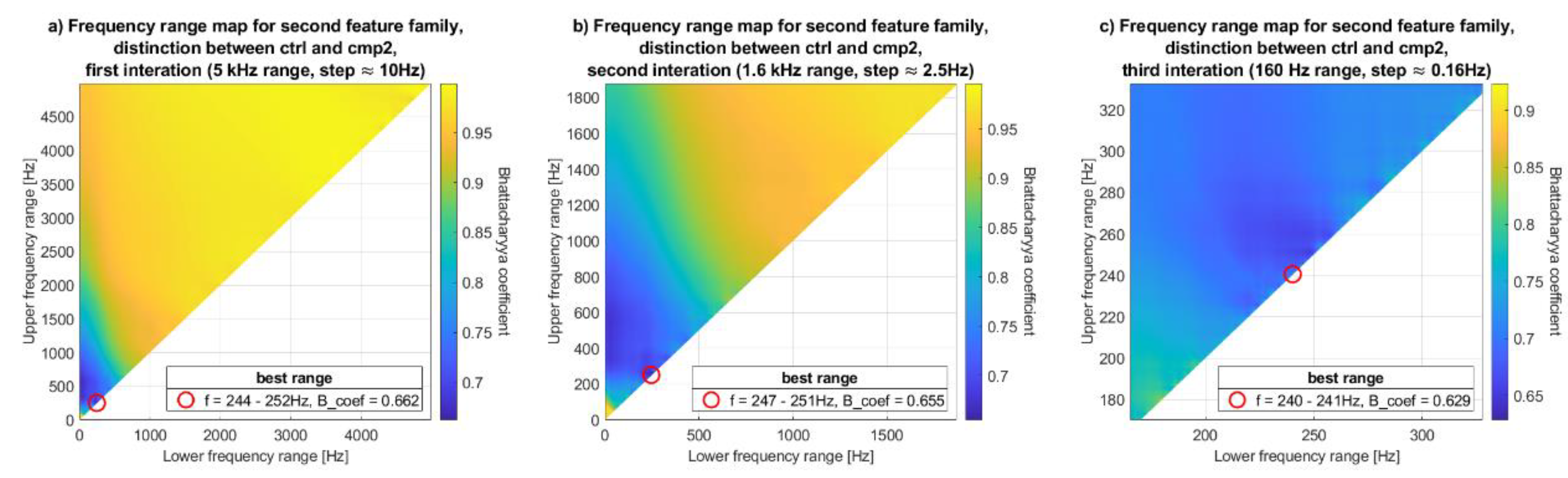
3.2. Optimal Frequency Range
3.3. Definition of the Features
- d1 is the first feature family,
- δf is the normalization factor, equal to the . It ensures that the value of the feature is affected only by the shape of the spectrum and not by its size,
- f1 is the lower frequency range,
- f2 is the upper frequency range,
- f2 is the upper frequency range,
- sVAG is the VAG signal,
- DFT is the Discrete Fourier Transform operator,
- fi is the i-th frequency amplitude.
4. Research Methodology
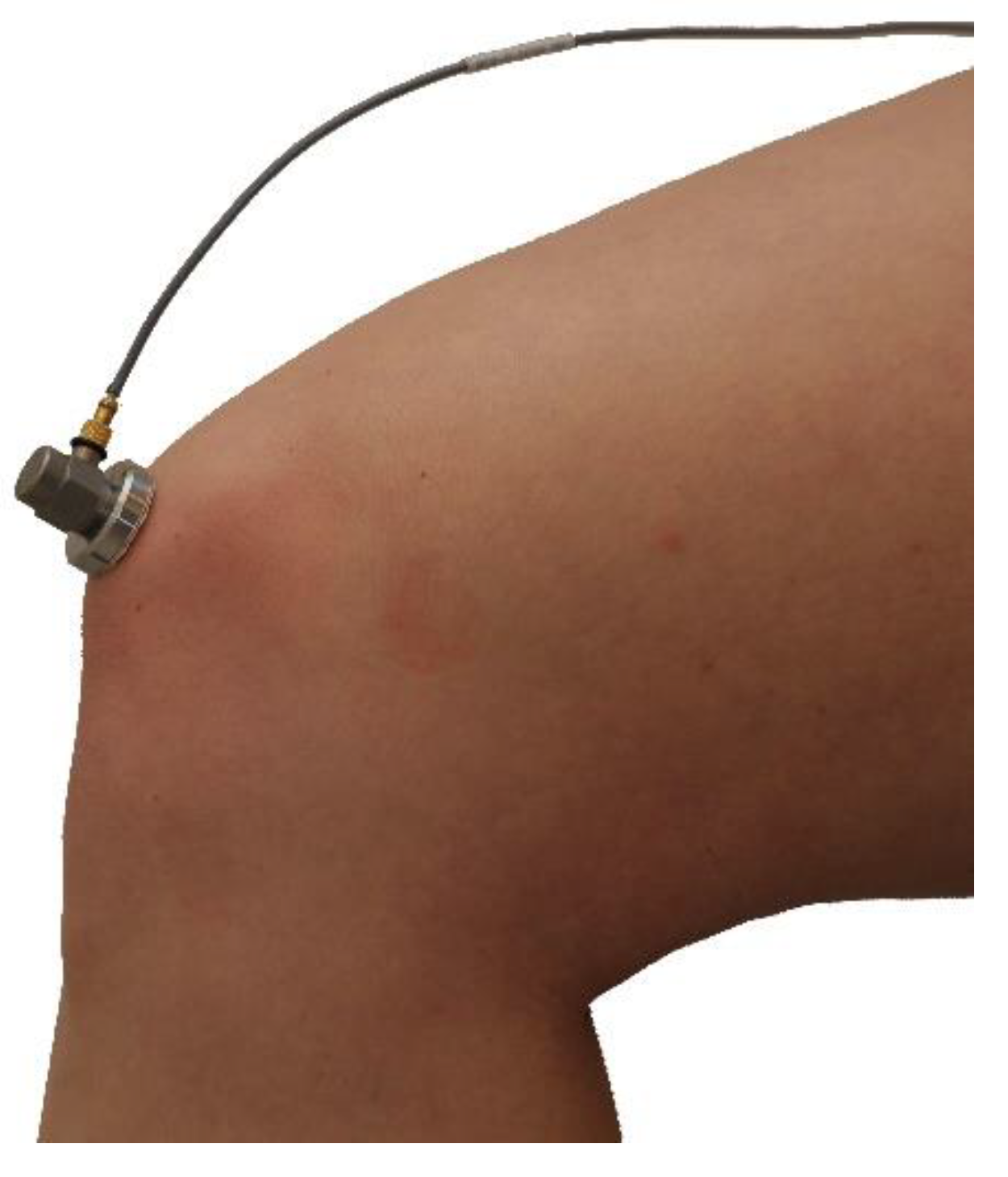
4.1. Acquisition of the VAG Signal
4.2. The Process of Defining New Frequency Features
- the DFT of the VAG signal, from which the first feature family is obtained, using Equation (3),
- the DFT of the derivative of the VAG signal, from which the second feature family is obtained, using Equation (5),
- squared DFT of the VAG signal, from which the third feature family is obtained, using Equation (6),
- squared DFT of the derivative of the VAG signal, from which the fourth feature family is obtained, using Equation (7).
- the first one in range 0–5 kHz (since signal was sampled with the frequency of 10 kHz), with about 10 Hz step. Features were then defined as sums, defined by Equations (3) and (5)–(7), in subsequent ranges: 0–10 Hz, 0–20 Hz, …, 0–5000 Hz, 10–20 Hz, 10–30 Hz, …, 4980–4990 Hz, 4980–5000 Hz, 4990–5000 Hz. Every range was evaluated by Bhattacharyya coefficient and plotted as a point on the FRM.
- the second iteration was conducted in range ±800 Hz from the best range obtained in previous iteration with about 2.5 Hz step,
- the last iteration was conducted in range ±80 Hz from the best range obtained in previous iteration with about 0.16 Hz step.
- that the found frequency ranges for each classes are as optimal as possible, without sacrificing the distinction between more different conditions (maybe one frequency range would be appropriate for the distinction between the first and the second stage chondromalacia, but not as effective with distinguishing between first stage chondromalacia and the osteoarthritis; the question would arise, which distinction should be dominant, and which should be sacrificed),
- that the obtained frequency ranges provide as unambiguous distinction as possible; the situation can be imagined in which two classes neighboring one another (for example cmp1 and cmp3 neighboring cmp2) can be distinguished from the one with very similar frequency ranges. Then the statement that the particular frequency range is typical for, e.g., cmp2 would be true, but the contrary would not unambiguously point out cmp1 or cmp3.
4.3. The Verification of Defined Features as a Classifier Input
5. Results and Discussion

| Boxplot Letter (Figure 7) | Class Combination | The Bhattacharyya Coefficient for Feature Family: | |||
|---|---|---|---|---|---|
| 1 (DFT of the Signal) | 2 (DFT of the Derivative) | 3 (Square of the DFT of the Signal) | 4 (Square of the DFT of the Derivative) | ||
| a | ctrl, cmp1 | 0.863 | 0.844 | 0.842 | 0.872 |
| b | ctrl, cmp2 | 0.634 | 0.629 | 0.659 | 0.662 |
| c | ctrl, cmp3 | 0.318 | 0.316 | 0.453 | 0.464 |
| d | ctrl, oa | 0.308 | 0.367 | 0.458 | 0.462 |
| e | cmp1, cmp2 | 0.726 | 0.717 | 0.769 | 0.768 |
| f | cmp1, cmp3 | 0.446 | 0.442 | 0.560 | 0.577 |
| g | cmp1, oa | 0.401 | 0.486 | 0.587 | 0.603 |
| h | cmp2, cmp3 | 0.637 | 0.667 | 0.694 | 0.693 |
| i | cmp2, oa | 0.594 | 0.696 | 0.741 | 0.744 |
| j | cmp3, oa | 0.900 | 0.919 | 0.897 | 0.876 |
| Boxplot Letter (Figure 7) | Class Combination | The Frequency Range (Hz) for Feature Family: | |||
|---|---|---|---|---|---|
| 1 (DFT of the Signal) | 2 (DFT of the Derivative) | 3 (Square of the DFT of the Signal) | 4 (Square of the DFT of the Derivative) | ||
| a | ctrl, cmp1 | 235.51–235.51 | 279.95–279.95 | 235.51–235.51 | 226.56–226.56 |
| b | ctrl, cmp2 | 240.23–240.56 | 240.23–240.56 | 331.22–331.38 | 331.22–331.38 |
| c | ctrl, cmp3 | 111.17–452.96 | 103.19–359.21 | 109.70–428.39 | 26.20–303.71 |
| d | ctrl, oa | 15.79–1110.68 | 0.00–554.85 | 47.69–5000.00 | 0.00–649.25 |
| e | cmp1, cmp2 | 398.11–398.93 | 405.76–405.76 | 258.3–258.63 | 239.10–239.10 |
| f | cmp1, cmp3 | 78.78–465.82 | 15.14–417.97 | 78.61–428.39 | 9.11–290.36 |
| g | cmp1, oa | 8.46–849.61 | 0.81–470.70 | 42.64–5000.00 | 0.81–690.92 |
| h | cmp2, cmp3 | 94.40–394.86 | 91.80–287.43 | 88.05–392.42 | 79.92–263.83 |
| i | cmp2, oa | 8.79–955.73 | 0.00–513.02 | 71.45–5000.00 | 233.40–233.89 |
| j | cmp3, oa | 0.00–4384.44 | 0.98–166.18 | 16.28–193.20 | 157.88–157.88 |
| Class Combination | Bhattacharyya Coefficient | |||||
|---|---|---|---|---|---|---|
| P1 (50–250 Hz) | P2 (250–450 Hz) | F470 (470 Hz) | F780 (780 Hz) | The Best Feature from Table 1 | Improvement (%) | |
| ctrl, cmp1 | 0.964 | 0.960 | 0.951 | 0.963 | 0.842 | 11.46 |
| ctrl, cmp2 | 0.906 | 0.795 | 0.924 | 0.943 | 0.659 | 17.11 |
| ctrl, cmp3 | 0.549 | 0.668 | 0.837 | 0.947 | 0.316 | 42.44 |
| ctrl, oa | 0.582 | 0.516 | 0.860 | 0.943 | 0.308 | 40.31 |
| cmp1, cmp2 | 0.942 | 0.874 | 0.936 | 0.904 | 0.717 | 17.96 |
| cmp1, cmp3 | 0.607 | 0.782 | 0.882 | 0.955 | 0.442 | 43.48 |
| cmp1, oa | 0.670 | 0.635 | 0.901 | 0.948 | 0.401 | 36.85 |
| cmp2, cmp3 | 0.809 | 0.881 | 0.952 | 0.965 | 0.637 | 21.26 |
| cmp2, oa | 0.809 | 0.809 | 0.950 | 0.951 | 0.594 | 26.58 |
| cmp3, oa | 0.924 | 0.962 | 0.985 | 0.980 | 0.876 | 5.19 |
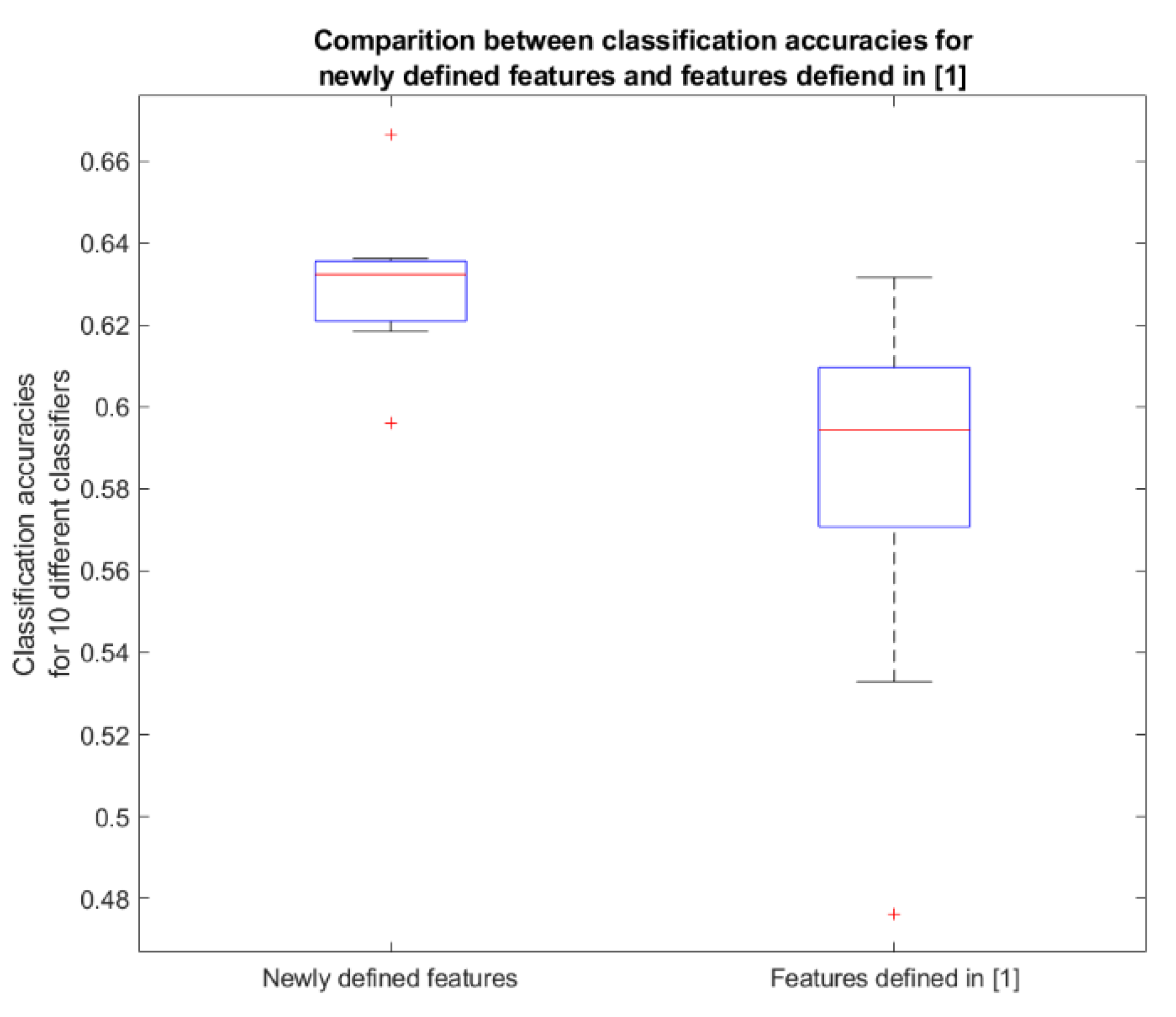
| No. | Classifier | Classification Accuracy | Additional info. about Classifier | ||
|---|---|---|---|---|---|
| The New Features | The Features Defined in [1] | Improvement (%) | |||
| 1 | decision tree | 0.62 | 0.59 | 5.1 | max. 10 splits |
| 2 | decision tree | 0.60 | 0.59 | 1.7 | max. 5 splits |
| 3 | discriminant analysis | 0.63 | 0.53 | 18.9 | |
| 4 | naïve Bayes | 0.64 | 0.48 | 33.3 | |
| 5 | support vector machine | 0.67 | 0.63 | 6.3 | linear kernel |
| 6 | k nearest neighbors | 0.64 | 0.61 | 4.9 | k = 20, euclidean distance |
| 7 | k nearest neighbors | 0.63 | 0.62 | 1.6 | k = 5, euclidean distance |
| 8 | decision forest | 0.62 | 0.57 | 8.8 | bagging |
| 9 | decision forest | 0.63 | 0.60 | 5.0 | boosting, max 10 splits |
| 10 | neural network | 0.63 | 0.60 | 5.0 | 10 hidden neurons, tansig function |
| mean | 0.63 | 0.58 | 9.1 | ||
| max | 0.67 | 0.63 | 33.3 | ||
6. Conclusions
Author Contributions
Funding
Conflicts of Interest
References
- Kręcisz, K.; Bączkowicz, D. Analysis and multiclass classification of pathological knee joints using vibroarthrographic signals. Comput. Methods Prog. Biomed. 2018, 154, 37–44. [Google Scholar] [CrossRef] [PubMed]
- Befrui, N.; Elsner, J.; Flesser, A.; Huvanandana, J.; Jarrousse, O.; Le, T.N.; Müller, M.; Schulze, W.H.W.; Taing, S.; Weidert, S. Vibroarthrography for early detection of knee osteoarthritis using normalized frequency features. Med. Biol. Eng. Comput. 2018, 56, 1499–1514. [Google Scholar] [CrossRef] [PubMed]
- Bączkowicz, D.; Kręcisz, K. Vibroarthrography in the evaluation of musculoskeletal system a pilot study. Ortop. Traumatol. Rehabil. 2013, 15, 407–416. [Google Scholar] [CrossRef] [PubMed]
- Bączkowicz, D.; Majorczyk, E. Joint motion quality in vibroacoustic signal analysis for patients with patellofemoral joint disorders. BMC Musculoskelet. Disord. 2014, 15, 426–433. [Google Scholar] [CrossRef] [Green Version]
- Bączkowicz, D.; Majorczyk, E.; Kręcisz, K. Age-related impairment of quality of joint motion in vibroarthrographic signal analysis. BioMed Res. Int. 2015, 2015, 1–7. [Google Scholar] [CrossRef] [Green Version]
- Bączkowicz, D.; Majorczyk, E. Joint motion quality in chondromalacia progression assessed by vibroacoustic signal analysis. PM R 2016, 8, 1065–1071. [Google Scholar] [CrossRef]
- Wu, Y. Knee Joint Vibrographic Signal Processing and Analysis; Springer: London, UK, 2015. [Google Scholar]
- Krishnan, S.; Rangayyan, R.M.; Bell, G.D.; Frank, C.B.; Ladly, K.O. Adaptive filtering, modelling, and classification of knee joint vibroarthrographic signals for non-invasive diagnosis of articular cartilage pathology. Med. Biol. Eng. Comput. 1997, 35, 677–684. [Google Scholar] [CrossRef]
- Moussavi, Z.M.K.; Rangayyan, R.M.; Bell, G.D.; Frank, C.B.; Ladly, K.O.; Zhang, Y.T. Screening of vibroarthrographic signals via adaptive segmentation and linear prediction modeling. IEEE Trans. Biomed. Eng. 1996, 43, 15–23. [Google Scholar] [CrossRef]
- Rangayyan, R.M.; Wu, Y.F. Screening of knee-joint vibroarthrographic signals using statistical parameters and radial basis functions. Med. Biol. Eng. Comput. 2008, 46, 223–232. [Google Scholar] [CrossRef]
- Wu, Y.; Chen, P.; Luo, X.; Huang, H.; Liao, L.; Yao, Y.; Wu, M.; Rangayyan, R.M. Quantification of knee vibroarthrographic signalirregularity associated with patellofemoral jointcartilage pathology based on entropy and envelopeamplitude measures. Comput. Methods Programs Biomed. 2016, 130, 1–12. [Google Scholar] [CrossRef]
- Andersen, R.E.; Arendt-Nielsen, L.; Madeleine, P. Knee joint vibroarthrography of asymptomatic subjects during loaded flexion-extension movements. Med. Biol. Eng. Comput. 2018, 56, 2301–2312. [Google Scholar] [CrossRef] [PubMed]
- Nalband, S.; Prince, A.A.; Agrawal, A. Entropy-based feature extraction and classification of vibroarthographic signal using complete ensemble empirical mode decomposition with adaptive noise. IET Sci. Meas. Technol. 2018, 12, 350–359. [Google Scholar] [CrossRef]
- Łysiak, A.; Froń, A.; Bączkowicz, D.; Szmajda, M. The new descriptor in processing of vibroacoustic signal of knee joint. IFAC PapersOnLine 2019, 52, 335–340. [Google Scholar] [CrossRef]
- Dołegowski, M.; Szmajda, M. Use of incremental decomposition and spectrogram in vibroacoustic signal analysis in knee joint disease examination. Przegląd Elektrotech. 2018, 7/2018, 162–166. [Google Scholar] [CrossRef]
- Rangayyan, R.M.; Wu, Y. Analysis of vibroarthrographic signals with features related to signal variability and radial-basis functions. Ann. Biomed. Eng. 2009, 37, 156–163. [Google Scholar] [CrossRef]
- Mascarenhas, E.; Nalband, S.; Fredo, A.R.J.; Prince, A. Analysis and Classification of Vibroarthrographic Signals using Tuneable ‘Q’ Wavelet Transform. In Proceedings of the 2020 7th International Conference on Signal Processing and Integrated Networks, Noida, India, 27–28 February 2020. [Google Scholar] [CrossRef]
- Nalband, S.; Valliappan, C.A.; Prince, A.A.; Agrawal, A. Time-frequency based feature extraction for the analysis of vibroarthographic signals. Comput. Electr. Eng. 2018, 69, 720–731. [Google Scholar] [CrossRef]
- Guyon, I.; Gunn, S.; Nikravesh, M.; Zadeh, L.A. (Eds.) Feature Extractoin. In Foundations and Aplications, 1st ed.; Springer: Heidelberg, Germany, 2006. [Google Scholar]
- Wild, C.J.; Pfannkuch, M.; Regan, M.; Horton, N.J. Towards more accessible conceptions of statistical inference: Conceptions of Statistical Inference. J. R. Stat. Soc. A 2011, 174, 247–295. [Google Scholar] [CrossRef]
- Nachkebia, N.; Alexander, M.; House, W.; North, H. The Simple Theory of Informal Rules. Math. Teach. Res. J. Online 2013, 6, 83–99. [Google Scholar]
- Rao, J.S.; Liu, H. Discordancy Partitioning for Validating Potentially Inconsistent Pharmacogenomic Studies. Sci. Rep. 2017, 7, 15169. [Google Scholar] [CrossRef] [PubMed]
- Pramono, R.X.A.; Imtiaz, S.A.; Rodriguez-Villegas, E. Evaluation of features for classification of wheezes and normal respiratory sounds. PLoS ONE 2019, 14, e0213659. [Google Scholar] [CrossRef] [PubMed] [Green Version]
- Jaccard, P. Distribution comparée de la flore alpine dans quelques régions des Alpes occidentales et orientales. Bull. Soc. Vaud. Sci. Nat. 1901, 37, 241–272. [Google Scholar]
- Kailath, T. The Divergence and Bhattacharyya Distance Measures in Signal Selection. IEEE Trans. Commun. 1967, 15, 52–60. [Google Scholar] [CrossRef]
- Bowman, A.W.; Azzalini, A. The Kernel Approach with S-Plus Illustrations. In Applied Smoothing Techniques for Data Analysis, 1st ed.; Oxford University Press: New York, NY, USA, 1997. [Google Scholar]
- Perera, J.R.; Gikas, P.D.; Bentley, G. The present state of treatments for articular cartilage defects in the knee. Ann. R. Coll. Surg. Engl. 2012, 94, 381–387. [Google Scholar] [CrossRef] [PubMed] [Green Version]
- Culvenor, A.G.; Engen, C.N.; Øiestad, B.E.; Engebretsen, L.; Risberg, M.A. Defining the presence of radiographic knee osteoarthritis: A comparison between the Kellgren and Lawrence system and OARSI atlas criteria. Knee Surg. Sports Traumatol. Arthrosc. 2015, 23, 3532–3539. [Google Scholar] [CrossRef] [PubMed]
- Wang, W.; Carreira-Perpiñán, M.Á. The role of dimensionality reduction in linear classification. arXiv 2014, arXiv:1405.6444. Available online: http://arxiv.org/abs/1405.6444 (accessed on 2 July 2020).


© 2020 by the authors. Licensee MDPI, Basel, Switzerland. This article is an open access article distributed under the terms and conditions of the Creative Commons Attribution (CC BY) license (http://creativecommons.org/licenses/by/4.0/).
Share and Cite
Łysiak, A.; Froń, A.; Bączkowicz, D.; Szmajda, M. Vibroarthrographic Signal Spectral Features in 5-Class Knee Joint Classification. Sensors 2020, 20, 5015. https://doi.org/10.3390/s20175015
Łysiak A, Froń A, Bączkowicz D, Szmajda M. Vibroarthrographic Signal Spectral Features in 5-Class Knee Joint Classification. Sensors. 2020; 20(17):5015. https://doi.org/10.3390/s20175015
Chicago/Turabian StyleŁysiak, Adam, Anna Froń, Dawid Bączkowicz, and Mirosław Szmajda. 2020. "Vibroarthrographic Signal Spectral Features in 5-Class Knee Joint Classification" Sensors 20, no. 17: 5015. https://doi.org/10.3390/s20175015