Automotive Radar in a UAV to Assess Earth Surface Processes and Land Responses

 ,
,  ,
, 
Abstract
:1. Introduction
2. Materials and Methods
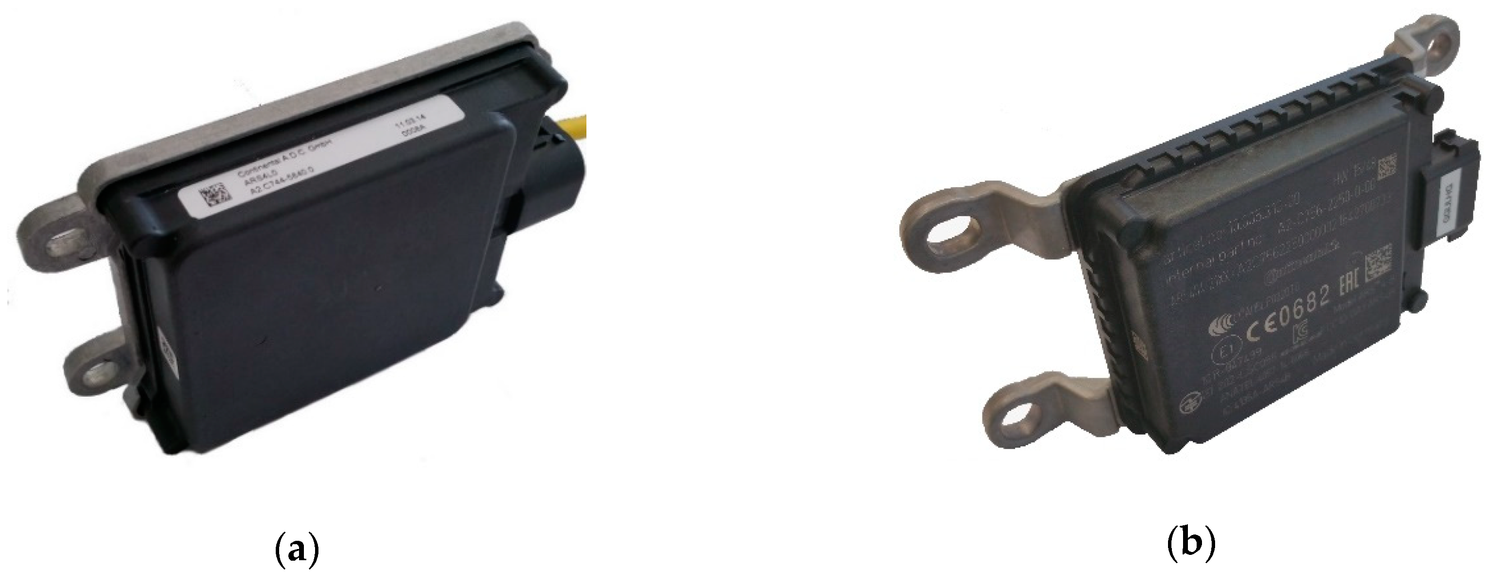
2.1. Automotive Radar Technology
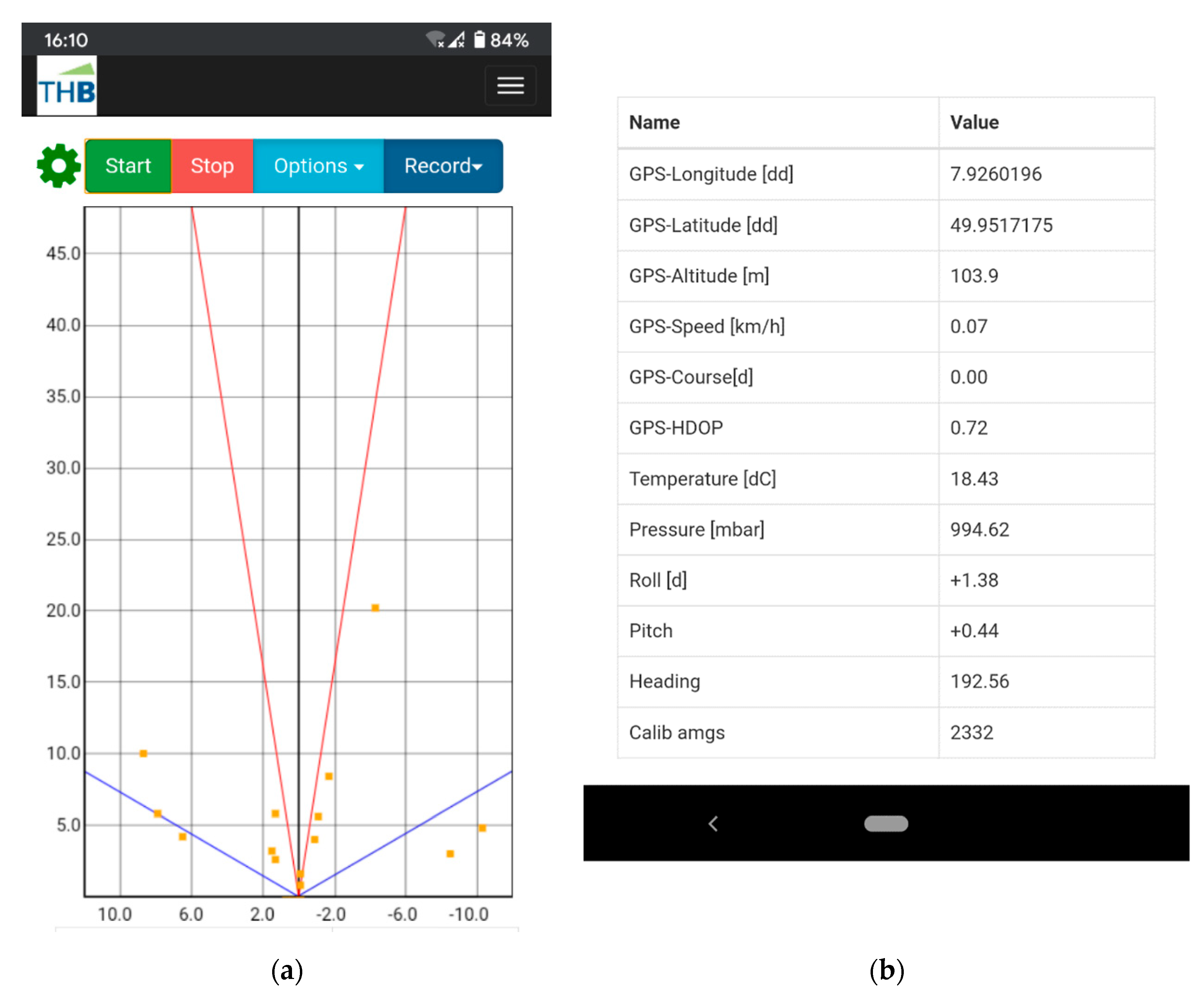
2.2. Recording System
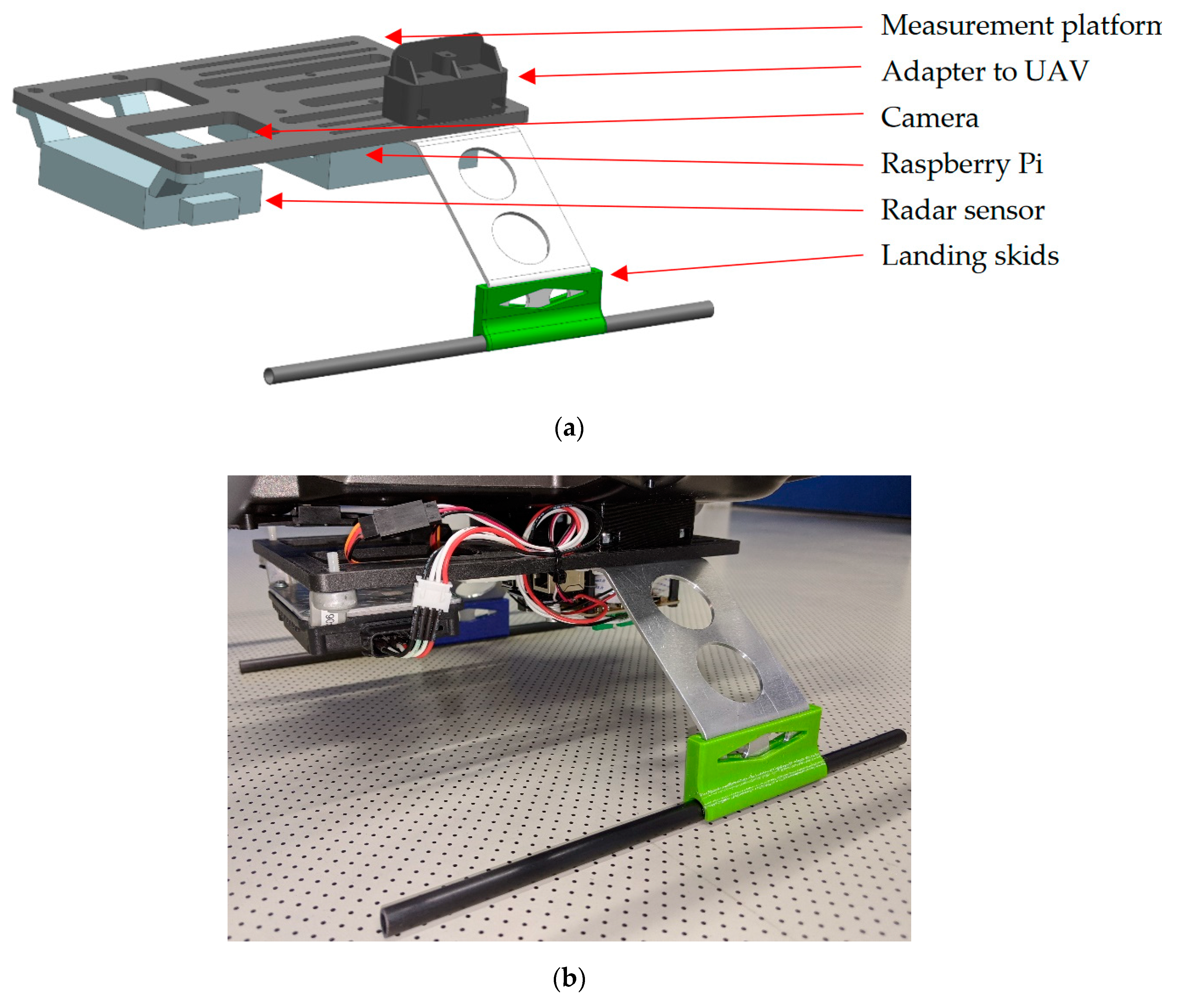
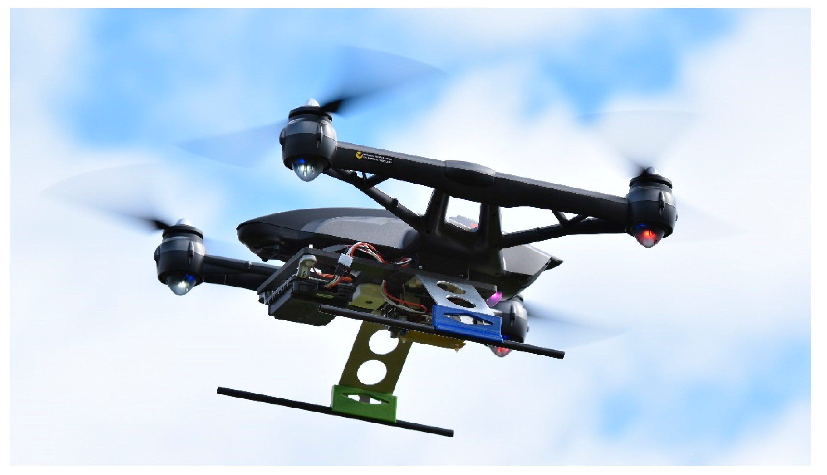
2.3. Integration in the UAV
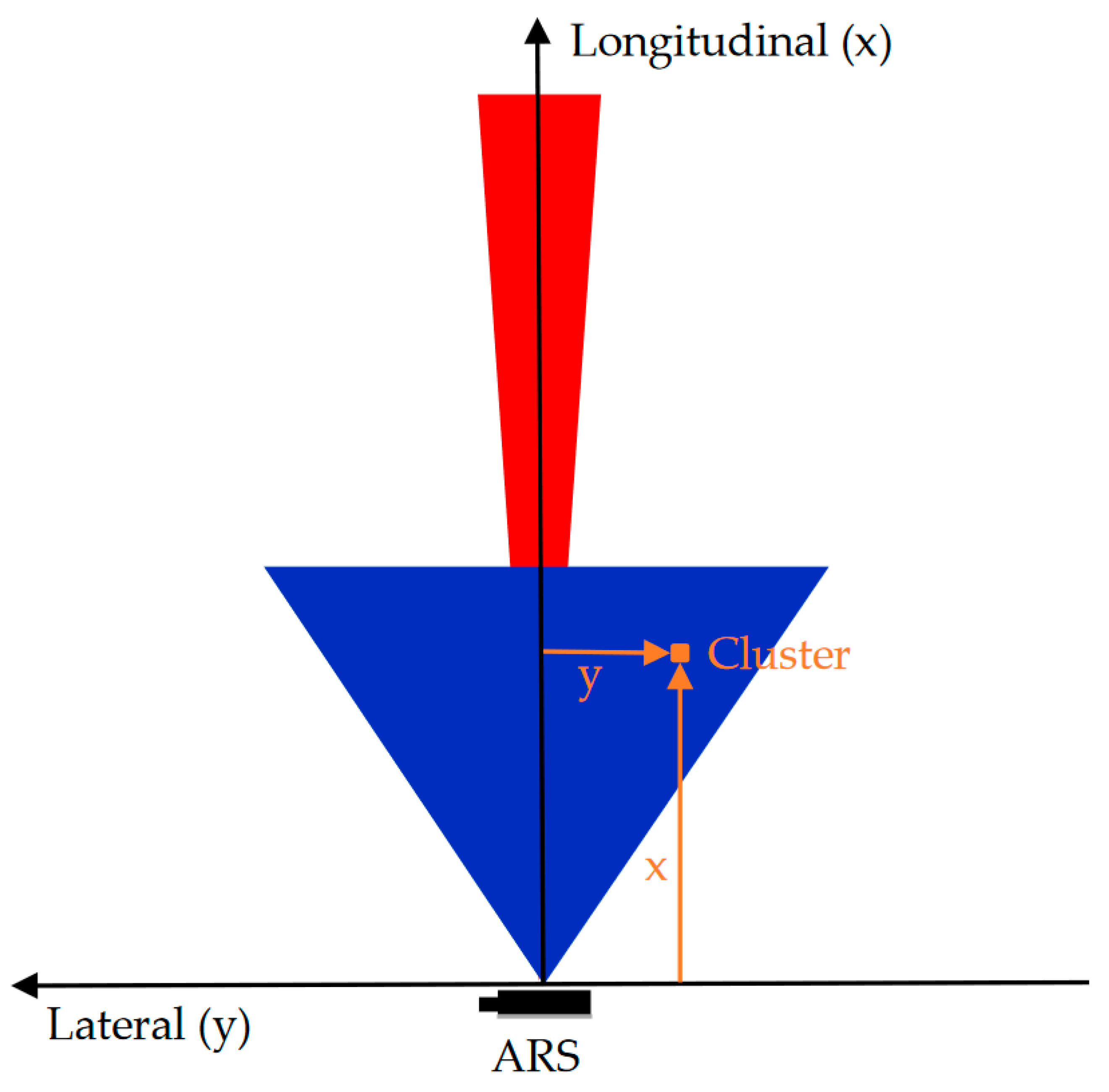
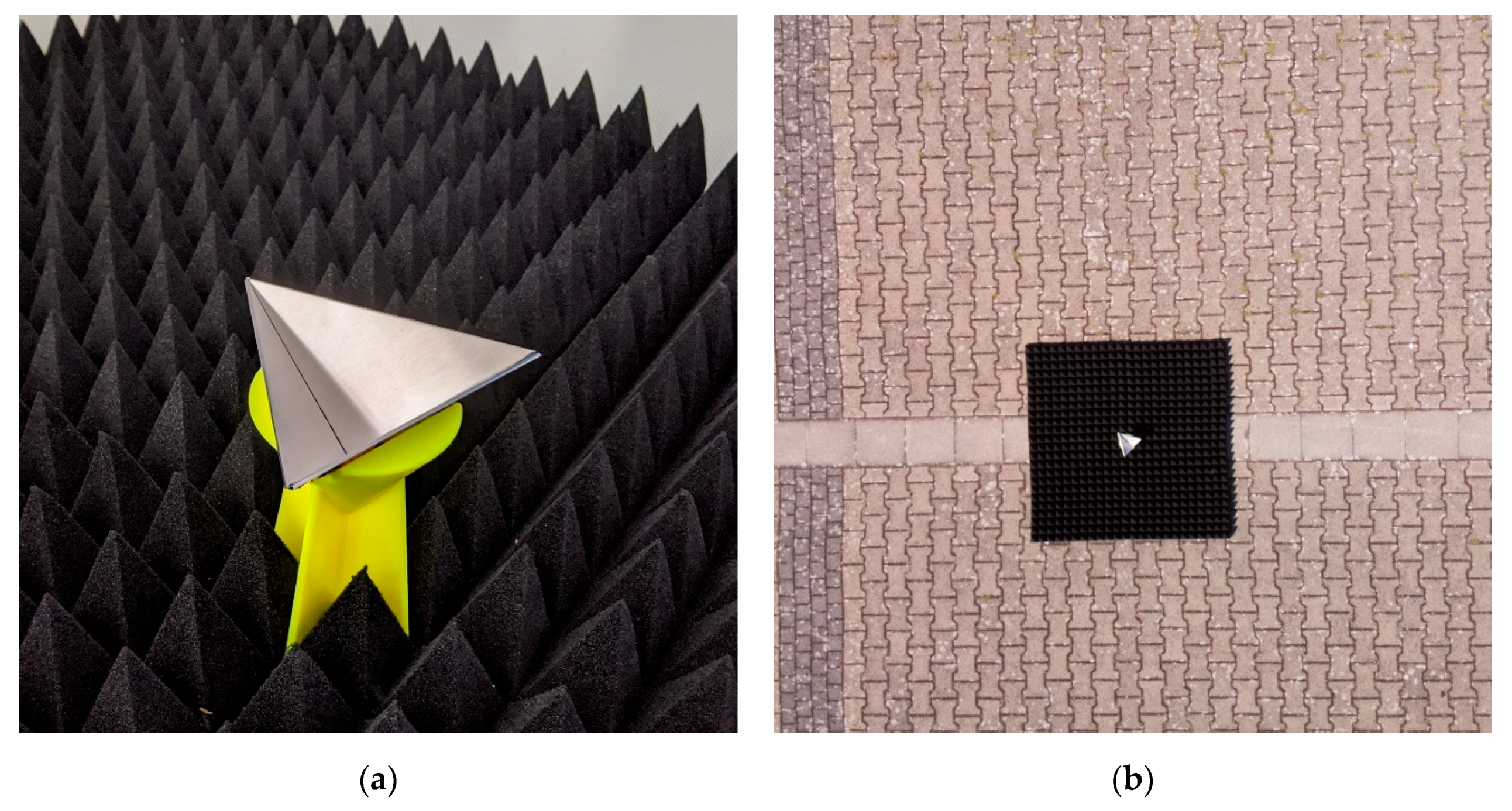
2.4. Radar Target
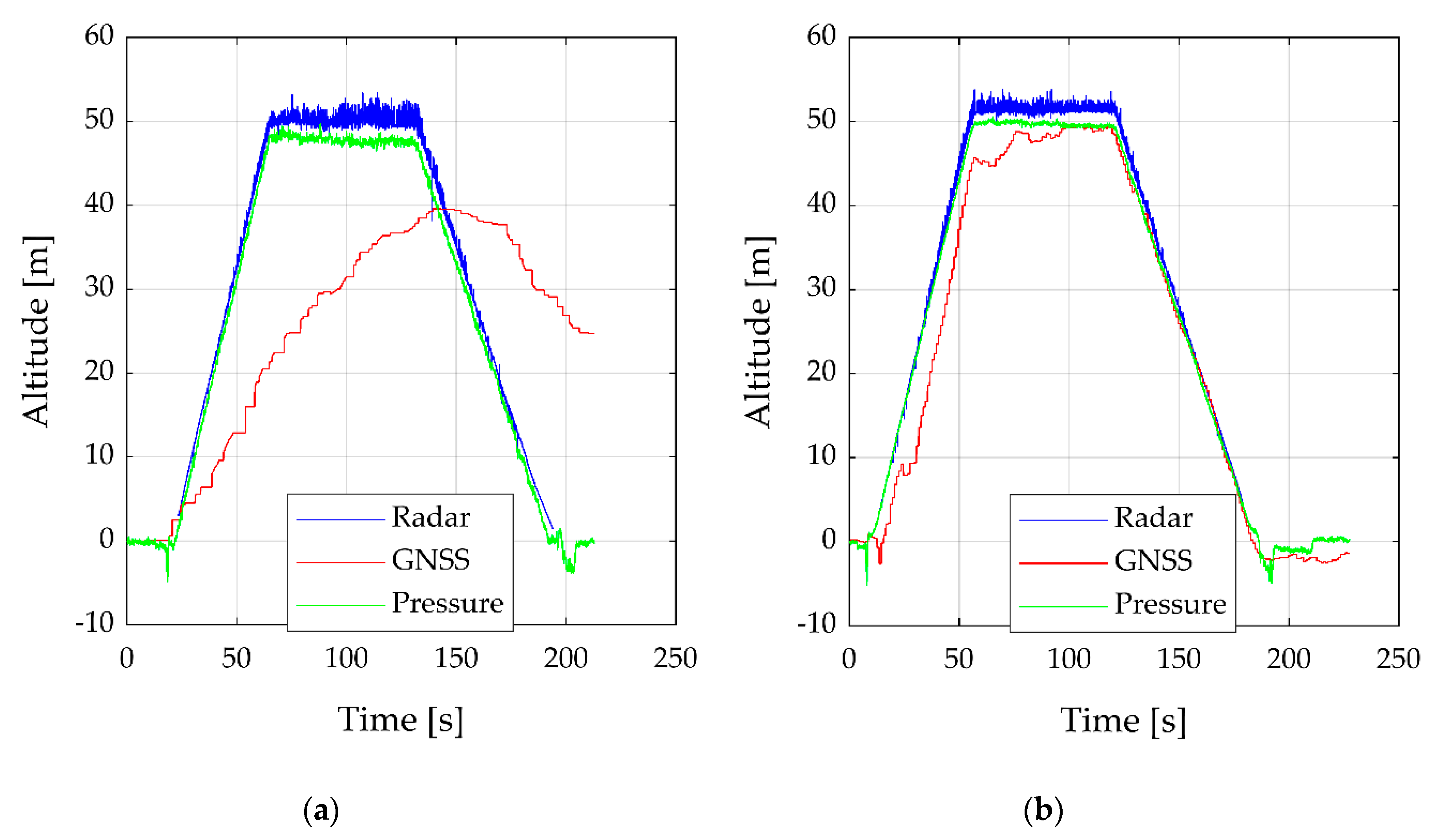
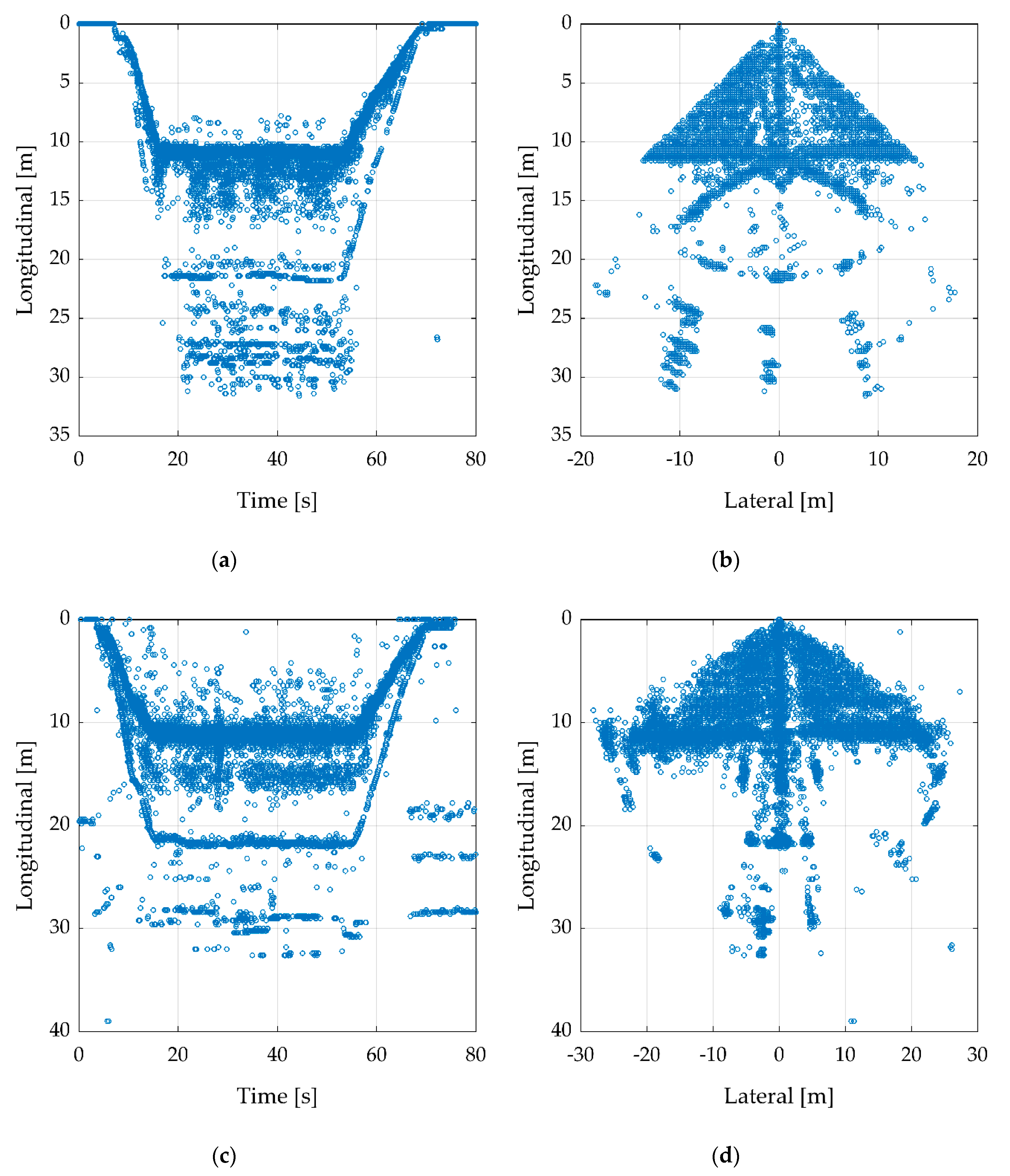
3. Results and Discussion
4. Conclusions
Author Contributions
Funding
Acknowledgments
Conflicts of Interest
References
- Colomina, I.; Molina, P. Unmanned aerial systems for photogrammetry and remote sensing: A review. ISPRS J. Photogramm. Remote Sens. 2014, 92, 79–97. [Google Scholar] [CrossRef] [Green Version]
- Aasen, H.; Honkavaara, E.; Lucieer, A.; Zarco-Tejada, P.J. Quantitative Remote Sensing at Ultra-High Resolution with UAV Spectroscopy: A Review of Sensor Technology, Measurement Procedures, and Data Correction Workflows. Remote Sens. 2018, 10, 1091. [Google Scholar] [CrossRef] [Green Version]
- Yin, N.; Liu, R.; Zeng, B.; Liu, N. A review: UAV-based Remote Sensing. IOP Conf. Ser. Mater. Sci. Eng. 2019, 490, 062014. [Google Scholar] [CrossRef]
- Jeziorska, J. UAS for Wetland Mapping and Hydrological Modeling. Remote Sens. 2019, 11, 1997. [Google Scholar] [CrossRef] [Green Version]
- Barbedo, J.G.A. A Review on the Use of Unmanned Aerial Vehicles and Imaging Sensors for Monitoring and Assessing Plant Stresses. Drones 2019, 3, 40. [Google Scholar] [CrossRef] [Green Version]
- Saito, H.; Uchiyama, S.; Hayakawa, Y.S.; Obanawa, H. Landslides triggered by an earthquake and heavy rainfalls at Aso volcano, Japan, detected by UAS and SfM-MVS photogrammetry. Prog. Earth Planet Sci. 2018, 5, 15. [Google Scholar] [CrossRef]
- Deguchi, T.; Sugiyama, T.; Kishimoto, M. Landslide monitoring by using ground-based millimeter wave radar system. In Proceedings of the ECSMGE 2019–XVII European Conference on Soil Mechanics and Geotechnical Engineering, Reykjavik, Iceland, 1–9 September 2019; pp. 627–632. [Google Scholar] [CrossRef]
- d’Oleire-Oltmanns, S.; Marzolff, I.; Peter, K.; Ries, J. Unmanned Aerial Vehicle (UAV) for Monitoring Soil Erosion in Morocco. Remote Sens. 2012, 4, 3390–3416. [Google Scholar] [CrossRef] [Green Version]
- Comino, J.R.; Keesstra, S.D.; Cerdà, A. Connectivity assessment in Mediterranean vineyards using improved stock unearthing method, LiDAR and soil erosion field surveys. Earth Surf. Process. Landf. 2018, 43, 2193–2206. [Google Scholar] [CrossRef]
- Garcia-Fernandez, M.; Alvarez-Lopez, Y.; Las Heras, F. Autonomous Airborne 3D SAR Imaging System for Subsurface Sensing: UWB-GPR on Board a UAV for Landmine and IED Detection. Remote Sens. 2019, 11, 2357. [Google Scholar] [CrossRef] [Green Version]
- Colorado, J.; Mondragon, I.; Rodriguez, J.; Castiblanco, C. Geo-Mapping and Visual Stitching to Support Landmine Detection Using a Low-Cost UAV. Int. J. Adv. Robot. Syst. 2015, 12, 125. [Google Scholar] [CrossRef] [Green Version]
- Wallace, L.; Lucieer, A.; Malenovský, Z.; Turner, D.; Vopěnka, P. Assessment of Forest Structure Using Two UAV Techniques: A Comparison of Airborne Laser Scanning and Structure from Motion (SfM) Point Clouds. Forests 2016, 7, 62. [Google Scholar] [CrossRef] [Green Version]
- Chen, Y.; Hakala, T.; Karjalainen, M.; Feng, Z.; Tang, J.; Litkey, P.; Kukko, A.; Jaakkola, A.; Hyyppä, J. UAV-Borne Profiling Radar for Forest Research. Remote Sens. 2017, 9, 58. [Google Scholar] [CrossRef] [Green Version]
- Al-Naji, A.; Perera, A.G.; Mohammed, S.L.; Chahl, J. Life Signs Detector Using a Drone in Disaster Zones. Remote Sens. 2019, 11, 2441. [Google Scholar] [CrossRef] [Green Version]
- Erdelj, M.; Natalizio, E.; Chowdhury, K.R.; Akyildiz, I.F. Help from the Sky: Leveraging UAVs for Disaster Management. IEEE Pervasive Comput. 2017, 16, 24–32. [Google Scholar] [CrossRef]
- Manfreda, S.; McCabe, M.; Miller, P.; Lucas, R.; Pajuelo Madrigal, V.; Mallinis, G.; Ben Dor, E.; Helman, D.; Estes, L.; Ciraolo, G.; et al. On the Use of Unmanned Aerial Systems for Environmental Monitoring. Remote Sens. 2018, 10, 641. [Google Scholar] [CrossRef] [Green Version]
- Yao, H.; Qin, R.; Chen, X. Unmanned Aerial Vehicle for Remote Sensing Applications—A Review. Remote Sens. 2019, 11, 1443. [Google Scholar] [CrossRef] [Green Version]
- Skolnik, M.I. Radar Handbook, 3rd ed.; McGraw-Hill: New York, NY, USA, 2008; ISBN 978-0-07-148547-0. [Google Scholar]
- Principles of Modern Radar; Richards, M.A.; Scheer, J.; Holm, W.A.; Melvin, W.L. (Eds.) SciTech Pub: Raleigh, NC, USA, 2010; ISBN 978-1-891121-52-4. [Google Scholar]
- Lacomme, P.; Hardange, J.-P.; Marchais, J.-C.; Normant, E. Air and Spaceborne Radar Systems: An Introduction; William Andrew Publishing: Norwich, NY, USA, 2001; ISBN 978-0-85296-981-6. [Google Scholar]
- Skolnik, M.I. Introduction to Radar Systems, 3rd International ed.; Mcgraw-Hill International Editions; Electrical Engineering Series; McGraw-Hill: Boston, MA, USA, 2000; ISBN 978-0-07-118189-1. [Google Scholar]
- Silicon Radar GmbH—Manufacturer of Radar Front Ends, MMICs, ASICs. Available online: https://siliconradar.com/ (accessed on 27 February 2020).
- Radarsensor for Industry and Automotive. Available online: https://www.innosent.de/en/index/ (accessed on 27 February 2020).
- Perna, S.; Alberti, G.; Berardino, P.; Bruzzone, L.; Califano, D.; Catapano, I.; Ciofaniello, L.; Donini, E.; Esposito, C.; Facchinetti, C.; et al. The ASI Integrated Sounder-SAR System Operating in the UHF-VHF Bands: First Results of the 2018 Helicopter-Borne Morocco Desert Campaign. Remote Sens. 2019, 11, 1845. [Google Scholar] [CrossRef] [Green Version]
- Shaw, J.B.; Ayoub, F.; Jones, C.E.; Lamb, M.P.; Holt, B.; Wagner, R.W.; Coffey, T.S.; Chadwick, J.A.; Mohrig, D. Airborne radar imaging of subaqueous channel evolution in Wax Lake Delta, Louisiana, USA. Geophys. Res. Lett. 2016, 43, 5035–5042. [Google Scholar] [CrossRef] [Green Version]
- Angelliaume, S.; Ceamanos, X.; Viallefont-Robinet, F.; Baqué, R.; Déliot, P.; Miegebielle, V. Hyperspectral and Radar Airborne Imagery over Controlled Release of Oil at Sea. Sensors 2017, 17, 1772. [Google Scholar] [CrossRef] [Green Version]
- Zhao, Q.; Lin, H.; Jiang, L.; Chen, F.; Cheng, S. A Study of Ground Deformation in the Guangzhou Urban Area with Persistent Scatterer Interferometry. Sensors 2009, 9, 503–518. [Google Scholar] [CrossRef]
- Ye, E.; Shaker, G.; Melek, W. Lightweight Low-Cost UAV Radar Terrain Mapping. In Proceedings of the 2019 13th European Conference on Antennas and Propagation (EuCAP), Krakow, Poland, 31 March–5 April 2019; pp. 1–5. [Google Scholar]
- Hugler, P.; Geiger, M.; Waldschmidt, C. 77 GHz radar-based altimeter for unmanned aerial vehicles. In Proceedings of the 2018 IEEE Radio and Wireless Symposium (RWS), Anaheim, CA, USA, 14–17 January 2018; IEEE: Piscataway, NL, USA, 2018; pp. 129–132. [Google Scholar]
- Schartel, M.; Burr, R.; Mayer, W.; Docci, N.; Waldschmidt, C. UAV-Based Ground Penetrating Synthetic Aperture Radar. In Proceedings of the 2018 IEEE MTT-S International Conference on Microwaves for Intelligent Mobility (ICMIM), Munich, Germany, 16 April 2018; IEEE: Piscataway, NL, USA, 2018; pp. 1–4. [Google Scholar]
- Handbook of Driver Assistance Systems: Basic Information, Components and Systems for Active Safety and Comfort; Winner, H.; Hakuli, S.; Lotz, F.; Singer, C. (Eds.) Springer International Publishing: Cham, Switzerland, 2016; ISBN 978-3-319-12351-6. [Google Scholar]
- Brakes, Brake Control and Driver Assistance Systems: Function, Regulation and Components; Reif, K. (Ed.) Bosch Professional Automotive Information; Springer Vieweg: Berlin, Germany, 2014; ISBN 978-3-658-03977-6. [Google Scholar]
- Wenger, J. Automotive radar—Status and perspectives. In Proceedings of the IEEE Compound Semiconductor Integrated Circuit Symposium, 2005. CSIC ’05, Palm Springs, CA, USA, 30 October–2 November 2005; IEEE: Piscataway, NL, USA; p. 4. [Google Scholar]
- Arabameri, A.; Cerda, A.; Pradhan, B.; Tiefenbacher, J.P.; Lombardo, L.; Bui, D.T. A methodological comparison of head-cut based gully erosion susceptibility models: Combined use of statistical and artificial intelligence. Geomorphology 2020, 359, 107136. [Google Scholar] [CrossRef]
- Rodrigo-Comino, J.; Wirtz, S.; Brevik, E.C.; Ruiz-Sinoga, J.D.; Ries, J.B. Assessment of agri-spillways as a soil erosion protection measure in Mediterranean sloping vineyards. J. Mt. Sci. 2017, 14, 1009–1022. [Google Scholar] [CrossRef]
- Wirtz, S.; Seeger, M.; Zell, A.; Wagner, C.; Wagner, J.-F.; Ries, J.B. Applicability of Different Hydraulic Parameters to Describe Soil Detachment in Eroding Rills. PLoS ONE 2013, 8, e64861. [Google Scholar] [CrossRef] [PubMed] [Green Version]
- Eltner, A.; Baumgart, P.; Maas, H.-G.; Faust, D. Multi-temporal UAV data for automatic measurement of rill and interrill erosion on loess soil. Earth Surf. Process. Landf. 2015, 40, 741–755. [Google Scholar] [CrossRef]
- Braud, I.; Borga, M.; Gourley, J.; Hürlimann, M.; Zappa, M.; Gallart, F. Flash floods, hydro-geomorphic response and risk management. J. Hydrol. 2016, 541, 1–5. [Google Scholar] [CrossRef] [Green Version]
- Otkin, J.A.; Svoboda, M.; Hunt, E.D.; Ford, T.W.; Anderson, M.C.; Hain, C.; Basara, J.B. Flash Droughts: A Review and Assessment of the Challenges Imposed by Rapid-Onset Droughts in the United States. Bull. Amer. Meteor. Soc. 2017, 99, 911–919. [Google Scholar] [CrossRef]
- Bertalan, L.; Rodrigo-Comino, J.; Surian, N.; Šulc Michalková, M.; Kovács, Z.; Szabó, S.; Szabó, G.; Hooke, J. Detailed assessment of spatial and temporal variations in river channel changes and meander evolution as a preliminary work for effective floodplain management. The example of Sajó River, Hungary. J. Environ. Manag. 2019, 248, 109277. [Google Scholar] [CrossRef]
- Barakat, M.; Mahfoud, I.; Kwyes, A.A. Study of soil erosion risk in the basin of Northern Al-Kabeer river at Lattakia-Syria using remote sensing andGIS techniques. Mesop. J. Mar. Sci. 2014, 29, 29–44. [Google Scholar]
- Gholami, H.; Telfer, M.W.; Blake, W.H.; Fathabadi, A. Aeolian sediment fingerprinting using a Bayesian mixing model. Earth Surf. Process. Landf. 2017, 42, 2365–2376. [Google Scholar] [CrossRef] [Green Version]
- Robichaud, P.R.; Jennewein, J.; Sharratt, B.S.; Lewis, S.A.; Brown, R.E. Evaluating the effectiveness of agricultural mulches for reducing post-wildfire wind erosion. Aeolian Res. 2017, 27, 13–21. [Google Scholar] [CrossRef]
- Amiri, F. Estimate of Erosion and Sedimentation in Semi-arid Basin using Empirical Models of Erosion Potential within a Geographic Information System. Air Soil Water Res. 2010, 3, ASWR.S3427. [Google Scholar] [CrossRef]
- Gutzler, C.; Helming, K.; Balla, D.; Dannowski, R.; Deumlich, D.; Glemnitz, M.; Knierim, A.; Mirschel, W.; Nendel, C.; Paul, C.; et al. Agricultural land use changes—A scenario-based sustainability impact assessment for Brandenburg, Germany. Ecol. Indic. 2015, 48, 505–517. [Google Scholar] [CrossRef] [Green Version]
- Martínez-Casasnovas, J.A.; Ramos, M.C.; García-Hernández, D. Effects of land-use changes in vegetation cover and sidewall erosion in a gully head of the Penedès region (northeast Spain). Earth Surf. Process. Landf. 2009, 34, 1927–1937. [Google Scholar] [CrossRef]
- Remke, A.; Rodrigo-Comino, J.; Gyasi-Agyei, Y.; Cerdà, A.; Ries, J.B. Combining the Stock Unearthing Method and Structure-from-Motion Photogrammetry for a Gapless Estimation of Soil Mobilisation in Vineyards. ISPRS Int. J. Geo-Inf. 2018, 7, 461. [Google Scholar] [CrossRef] [Green Version]
- CES–Industrial Radar Sensors–Adapted High Automotive Standard Radar Sensors for Object Detection in the Industry Application—Continental Engineering Services. Available online: https://www.conti-engineering.com/en-US/Industrial-Sensors/Sensors-Overview (accessed on 18 March 2020).
- Liebske, R. Short Description ARS 404-21 (Entry) + ARS 408-21 (Premium) Long Range Radar Sensor 77 GHz Technical Data; Continental: Hanover, Germany, 2016. [Google Scholar]
- von Eichel-Streiber, J.; Weber, C.; Rodrigo-Comino, J.; Altenburg, J. Controller for a Low-Altitude Fixed-Wing UAV on an Embedded System to Assess Specific Environmental Conditions. Available online: https://www.hindawi.com/journals/ijae/2020/1360702/ (accessed on 1 July 2020).
- Cox, T.J.; D’Antonio, P. Acoustic Absorbers and Diffusers: Theory, Design and Application; CRC Press: Boca Raton, FL, USA, 2009; ISBN 978-0-203-89305-0. [Google Scholar]
- Rossi, G.; Tanteri, L.; Tofani, V.; Vannocci, P.; Moretti, S.; Casagli, N. Multitemporal UAV surveys for landslide mapping and characterization. Landslides 2018, 15, 1045–1052. [Google Scholar] [CrossRef] [Green Version]
- Al-Rawabdeh, A.; Moussa, A.; Foroutan, M.; El-Sheimy, N.; Habib, A. Time Series UAV Image-Based Point Clouds for Landslide Progression Evaluation Applications. Sensors 2017, 17, 2378. [Google Scholar] [CrossRef] [Green Version]
- Salmoral, G.; Rivas-Casado, M.; Muthusamy, M.; Butler, D.; Menon, P.; Leinster, P. Guidelines for the Use of Unmanned Aerial Systems in Flood Emergency Response. Water 2020, 12, 521. [Google Scholar] [CrossRef] [Green Version]
- Lee, I.; Kang, J.; Seo, G. Applicability analysis of ultra-light uav for flooding site survey in south korea. In Proceedings of the ISPRS-International Archives of the Photogrammetry, Remote Sensing and Spatial Information Sciences, Hannover, Germany, 30 June 2013; Copernicus GmbH: Göttingen, Germany, 2013; Volume XL-1-W1, pp. 185–189. [Google Scholar]
- Rusnák, M.; Sládek, J.; Pacina, J.; Kidová, A. Monitoring of avulsion channel evolution and river morphology changes using UAV photogrammetry: Case study of the gravel bed Ondava River in Outer Western Carpathians. Area 2019, 51, 549–560. [Google Scholar] [CrossRef]
- Assessing Water Erosion Processes in Degraded Area Using Unmanned Aerial Vehicle Imagery. Available online: https://www.scielo.br/scielo.php?script=sci_arttext&pid=S0100-06832019000100525 (accessed on 23 July 2020).
- Yuan, M.; Zhang, Y.; Zhao, Y.; Deng, J. Effect of rainfall gradient and vegetation restoration on gully initiation under a large-scale extreme rainfall event on the hilly Loess Plateau: A case study from the Wuding River basin, China. Sci. Total Environ. 2020, 739, 140066. [Google Scholar] [CrossRef]
- Česnulevičius, A.; Bautrėnas, A.; Bevainis, L.; Ovodas, D.; Papšys, K. Applicability of Unmanned Aerial Vehicles in Research on Aeolian Processes. Pure Appl. Geophys. 2018, 175, 3179–3191. [Google Scholar] [CrossRef]
- Pijl, A.; Reuter, L.E.H.; Quarella, E.; Vogel, T.A.; Tarolli, P. GIS-based soil erosion modelling under various steep-slope vineyard practices. CATENA 2020, 193, 104604. [Google Scholar] [CrossRef]


| Specification | ARS-404 | ARS-408 |
|---|---|---|
| Voltage | +8.0 … 32 V DC | +8.0 … 32 V DC |
| Current | 375 mA by 12 V | 550 mA by 12 V |
| Power consumption | 4.5 W | 6.6 W |
| Weight | 172 g | 320 g |
| Size | 136 × 68 × 34 mm | 137 × 91 × 31 mm |
| Interface | High-Speed CAN | |
| Refresh rate | 50 ms | 60 ms |
| Range far/near area | 170 m/70 m | 250 m/70 m |
| Resolution far/near area | 0.4 m/0.4 m | 1.79 m/0.39 m |
| Beam horizontal far/near area | ±9°/±45° | ±9°/±60° |
| Resolution horizontal far/near area | 3.3°/6.6° | 1.6°/3.2° |
| Beam vertical far/near area | ±18°/±18° | ±14°/±20° |
| Frequency | 76–77 GHz | |
| Wavelength | 3.94–3.89 mm | |
| Cost (approx.) | €2500 | |
| Name | GPS-IMU v3 | GPS-PIE Gmm Slice |
|---|---|---|
| GNSS | uBlox CAM-M8 | GlobalTop Gmm-u1 |
| IMU | STMicroelectronics LSM9DS1 | Bosch BNO055 |
| Pressure and Temperature | Bosch BMP280/388 | TE Connectivity MS5637 |
| Manufacturer | OzzMaker, PO Box Q326, Queen Victoria Building, NSW 1230 Australia; ozzmaker.com | The BlackBoxCamera, Office 102, 61 Willow Walk, Tower Bridge, London SE1 5SF, United Kingdom; gps-pie.com |
| Cost | AUD$62.00 | £22.99 |
| Name | Type | Weight |
|---|---|---|
| Raspberry Pi with shields | 3B | 106 g |
| Raspberry Camera | Camera V2 | 4 g |
| Radar sensor | ARS-404 | 151 g |
| Radar sensor | ARS-408 | 296 g |
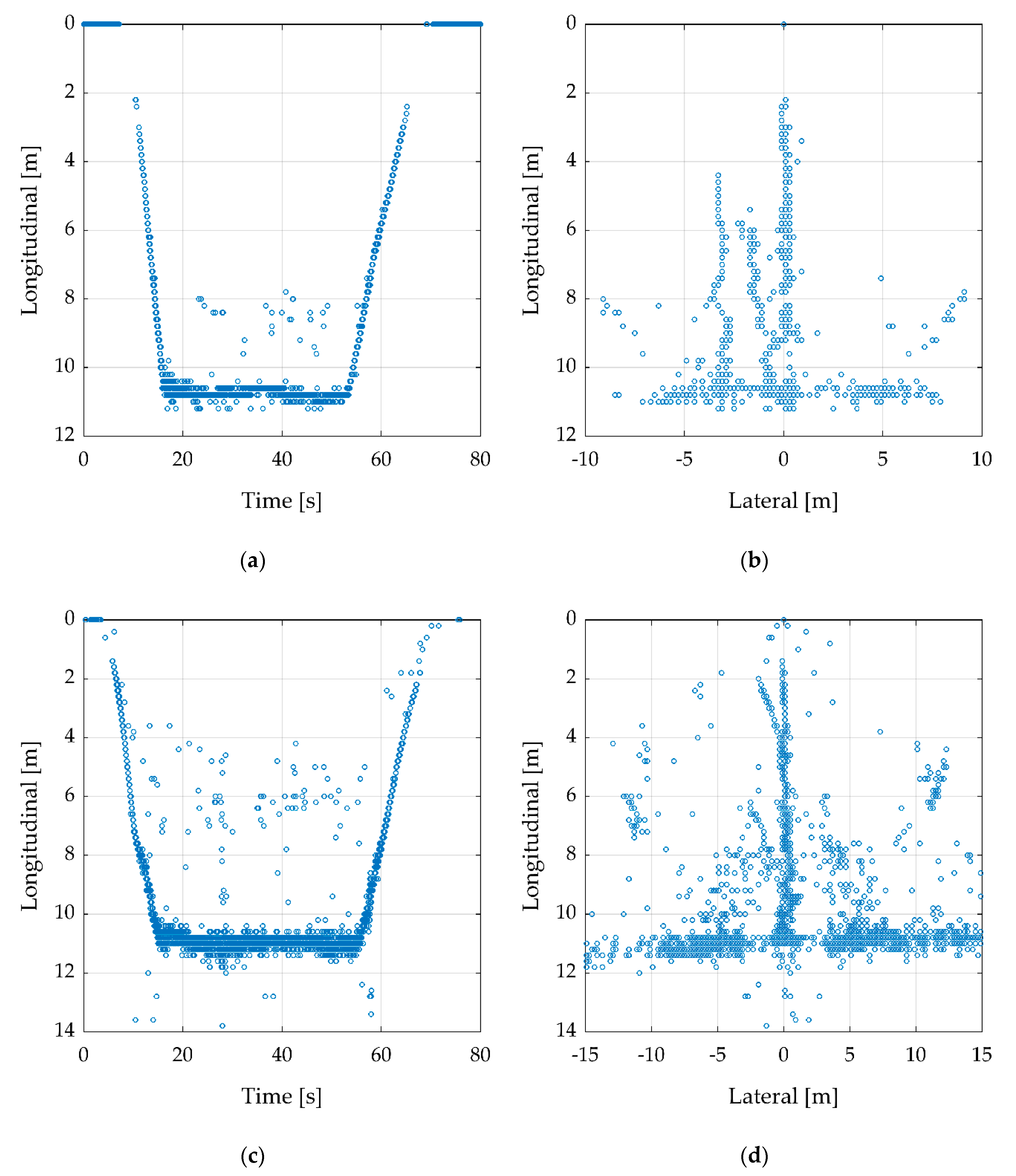
| Specification | Min | Max |
|---|---|---|
| Longitudinal | - | 20 m |
| Lateral | -15 m | 15 m |
| RCS | 0 m2 | - |
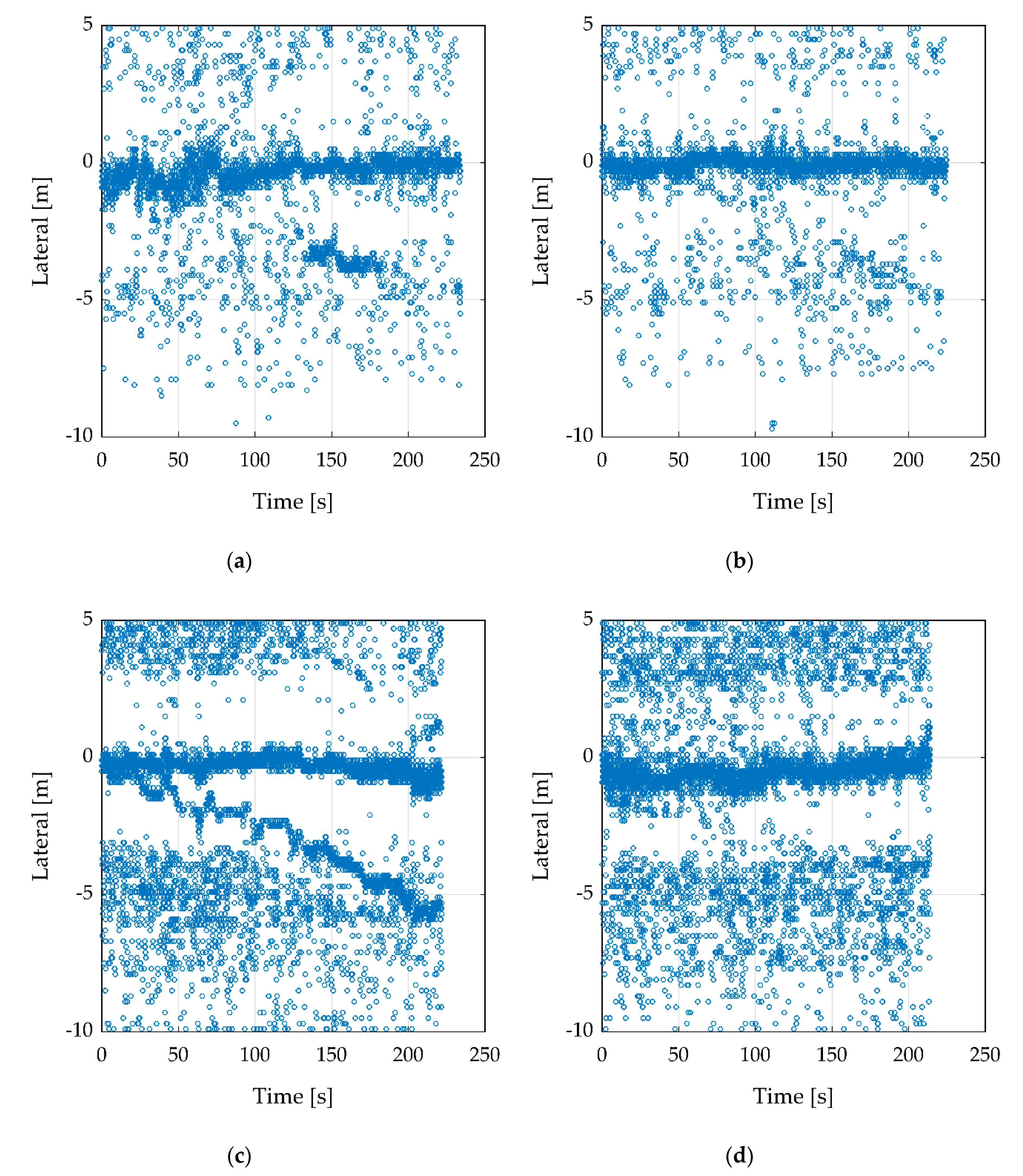
| Specification | Min | Max |
|---|---|---|
| Longitudinal | 20 m | |
| Lateral | −10 m | 5 m |
| RCS | 0 m2 |
© 2020 by the authors. Licensee MDPI, Basel, Switzerland. This article is an open access article distributed under the terms and conditions of the Creative Commons Attribution (CC BY) license (http://creativecommons.org/licenses/by/4.0/).
Share and Cite
Weber, C.; von Eichel-Streiber, J.; Rodrigo-Comino, J.; Altenburg, J.; Udelhoven, T. Automotive Radar in a UAV to Assess Earth Surface Processes and Land Responses. Sensors 2020, 20, 4463. https://doi.org/10.3390/s20164463
Weber C, von Eichel-Streiber J, Rodrigo-Comino J, Altenburg J, Udelhoven T. Automotive Radar in a UAV to Assess Earth Surface Processes and Land Responses. Sensors. 2020; 20(16):4463. https://doi.org/10.3390/s20164463
Chicago/Turabian StyleWeber, Christoph, Johannes von Eichel-Streiber, Jesús Rodrigo-Comino, Jens Altenburg, and Thomas Udelhoven. 2020. "Automotive Radar in a UAV to Assess Earth Surface Processes and Land Responses" Sensors 20, no. 16: 4463. https://doi.org/10.3390/s20164463