1. Introduction
Traffic congestion has caused a series of severe negative impacts like longer waiting time, more gas cost, and severe air pollution. According to a report in 2014 [
1], the loss caused by traffic jams is up to
$124 billion US dollars a year in the US. The shortage of traffic infrastructures, the growing number of vehicles, and the inefficient traffic signal control are key underlying reasons for traffic congestion. Among these, the traffic light control problem seems to be the most easily solved. However, the internal operation of the real urban transportation environment cannot be accurately calculated and analyzed mathematically due to its complexity and uncertainty. Reinforcement learning (RL), which is characterized by being data-driven, mode-less, and self-learning, is well suited for conducting research on adaptive traffic light control algorithms [
2,
3,
4].
The rapid development of artificial intelligence technology and deep learning (DL) has played a vital role in many fields. In recent years, DL has gained great success in image classification [
5,
6,
7,
8], machine translation [
9,
10,
11,
12], healthcare [
13], smart city [
14], time-series forecast [
15], Game of Go [
16] etc. The intelligent transportation systems (ITS) also have benefited from the latest AI achievement.
Traditional adaptive traffic light control method [
2,
3] could achieve local optimization by adapting to single intersection based on RL. Furthermore, global optimization is needed to achieve dynamic multi-intersection control in large smart city infrastructure. Multi-agent reinforcement learning (MARL) is increasingly being used to study more complex traffic light control issues [
17,
18,
19].
Although the existing methods have effectively improved the control efficiency of traffic signal control, they still have the following problems: (1) shortage of communication between a traffic light and other traffic lights; (2) shortage of consideration of the limitations of the capabilities of network transmission bandwidth. The contributions of this paper are summarized as the following:
We present an auto communication protocol (ACP) between agents in MARL based on attention mechanism;
We propose a multi-agent auto communication (MAAC) algorithm based on MARL and ACP in traffic light control;
We build a practicable edge computing architecture for industrial deployment on Internet of Things (IoT), considering the limitations of the capabilities of network transmission bandwidth;
The experiments show the MAAC framework outperformed 17 %over baseline models.
The remainder of this paper is organized as follows:
Section 2 introduces related works including multi-agent system, RL, IoT, edge computing, and the basic concept of communication theory.
Section 3 formulates the definition of the traffic light control problem.
Section 4 details the MAAC model and our edge computing architecture for IoT.
Section 5 conducts the experiments in a traffic simulation environment and demonstrates the results of the experiments with a comparison between our methods and others.
Section 6 concludes the paper and discusses future work.
2. Related Work
Urban traffic signal control theory has been continuously investigated and developed for nearly 70 years since the 1950s. However, from theory to practice, the goal of alleviating urban traffic congestion through the optimization and control of urban traffic signals, is consisting in very complex control problems. Urban traffic signal control is to allocate the time of a signal cycle and the ratio of the time of red and green lights in a signal cycle. The control methods include fixed time [
20], vehicle detection [
21], and automatic control [
22]. The fixed time and vehicle detection methods cannot adapt to the dynamic changes in traffic flow and complex road conditions. The automatic control methods are difficult to implement for its high algorithm complexity.
A multi-agent system is an important branch of distributed AI research, with the ability of distribution, autonomy, coordination, learning, and reasoning [
23]. In 1989, Durfee et al. [
24] proposed the use of a negotiation mechanism to share tasks among multiple agents. In 2007, Marvin Minsky argued that human thoughts were constructed by multi-agents [
25]. In 2016, Sukhbaatar et al. [
18] and Hoshen et al. [
19] observed all agents using a centrally controlled method in local environment, and then output the probability distribution of multi-agents’ joint actions. Alibaba and University College London (UCL) proposed the use of two-way communication network between agents network (BiNet) [
26], and achieved good results in the StarCraft game mission in 2017. From the trend of the multi-agent system, communication between agents has gotten more and more attention.
Adaptive traffic light control [
2,
3] is a relatively easy way to ease the traffic jam for smart city. Although adaptive traffic light control methods have achieved local optimization by adapting to single intersection based on RL (single-agent), the city has thousands of traffic lights. Thus, the global traffic light optimization could be considered as a multi-agent system, which has been studied by Chen et al. [
27]. Moreover, the deployment structure must be taken into consideration for the industrial deployment.
Here is the summary of the methods of traffic signal control (as
Table 1 shown):
2.1. Reinforcement Learning
2.1.1. Single-Agent Reinforcement Learning
Single-agent reinforcement learning was developed to train one agent, which chose a series of actions to get more rewards after interacting with an environment. To learn an optimal policy for the agent to gain maximal reward is the aim of the algorithm. At each time step t, the agent interacts with the environment to maximize the total reward , where T is the total number of time steps of an episode until it finishes. The rewards obtained after each action being performed are accumulated, which would be: .
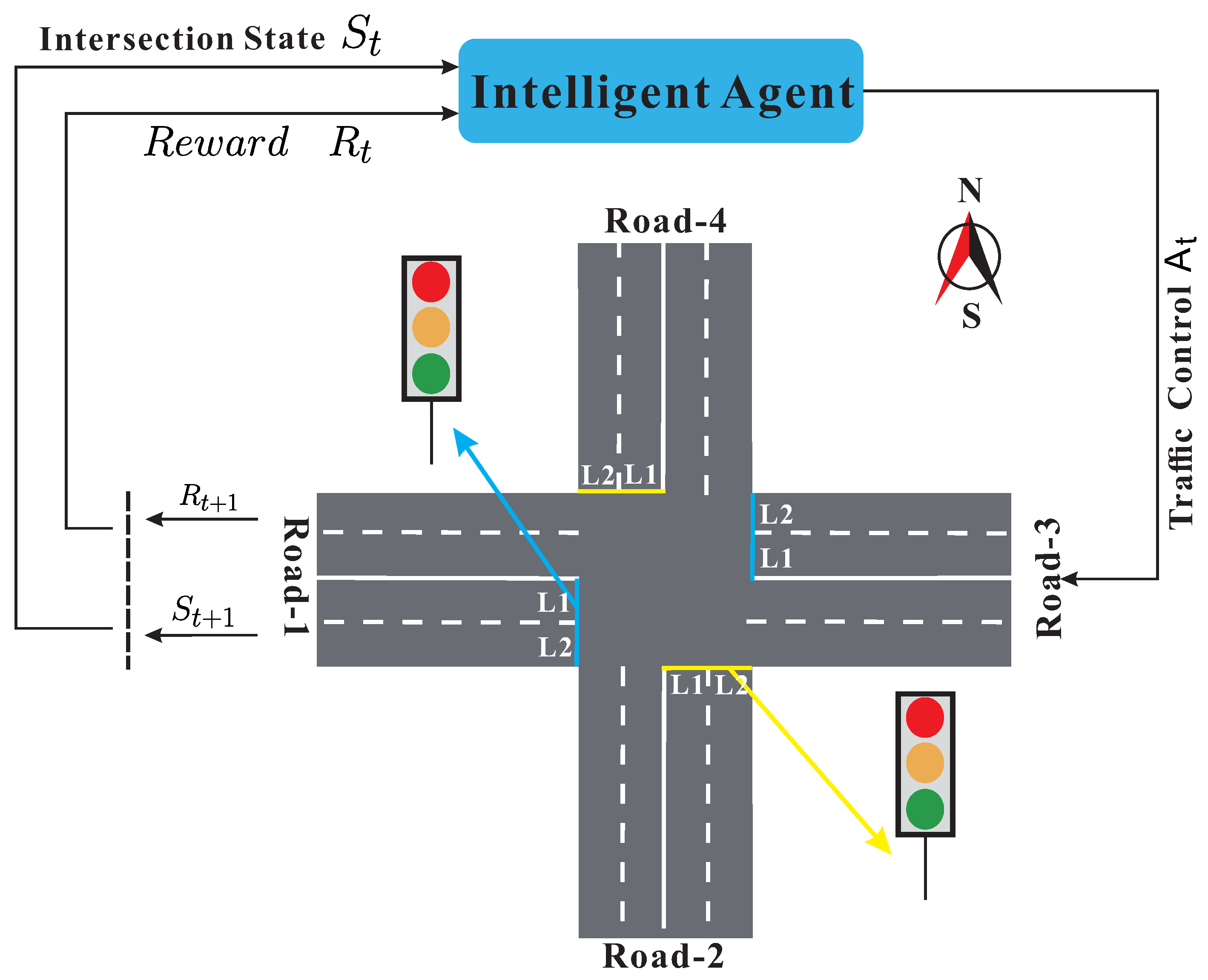
RL algorithm, which has the characteristics of “data-driven, self-learning, and model-free”, is considered to be a practical method to solve problem of traffic light control [
28,
29]. As shown in
Figure 1.
The traffic signal is regarded as an “agent” with decision-making ability at the intersection. By observing the real-time traffic flow, the current traffic status and the reward is obtained. According to the current status, the agent selects and executes the corresponding action (change lights or keep). Then, the agent observes the effect of the action on the intersection traffic to obtain the new traffic state and the new reward . The agent evaluates the action just selected so that it executes, optimizes strategies until converging to the optimal “state and action”.
2.1.2. Multi-Agent Reinforcement Learning
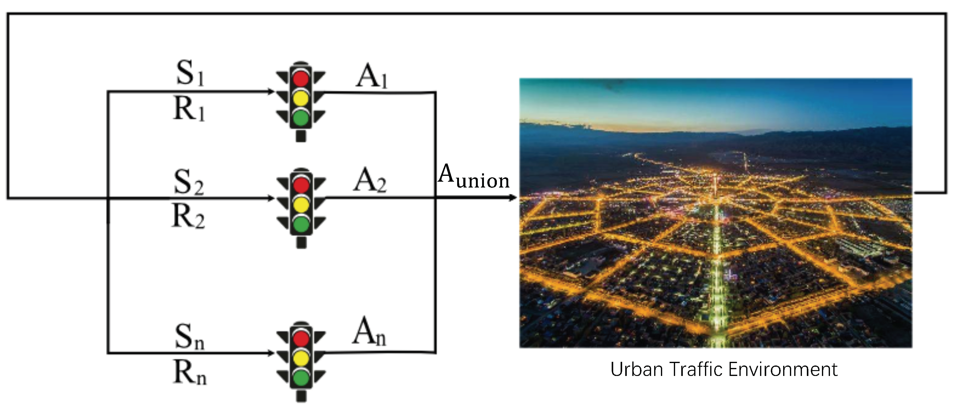
All agents apply their actions to the environment for whole rewards. From this perspective, we define a multi-agent reinforcement learning (MARL) environment as a tuple
where
is any given agent and
is any given action, then the new state of the environment is the result of a set of joined actions defined by
. In other words, the complexity of MARL scenarios increases with the number of agents in the environment (as shown in
Figure 2).
The urban traffic signal control can be seen as a typical multi-agent system. With the traditional adaptive traffic signal control method based on RL, the new signal controls have been expanded from one intersection to multiple intersections.
MARL is mainly to study the cooperative and coordinated control actions of multiple states of intersections, which extend the single-agent RL algorithm to multi-agents in the urban traffic environment. The MARL based methods in this field are divided into three categories [
30]: (1) a completely independent MARL at each intersection; (2) MARL in cooperation with some states from the intersections; (3) MARL in all states from the intersections.
The collaboration mechanism is an important part of MARL in traffic signal control at multiple intersections. Each agent could estimate the action probability model of other agents without real-time computing, but it was still difficult to update the estimation model in a dynamic environment [
31].
2.2. Attention Mechanism
Attention mechanism has recently been widely used in various fields of deep learning (for example, image processing [
32], natural language processing [
12,
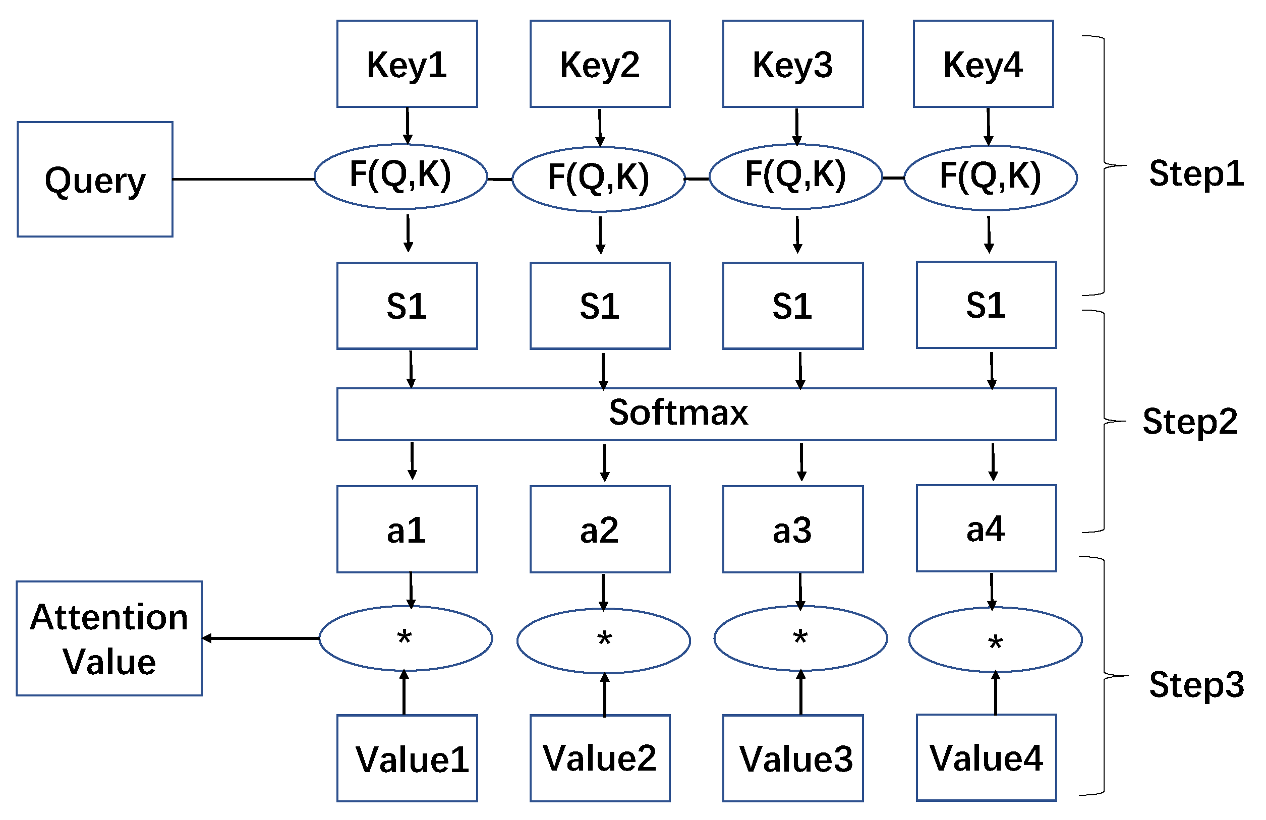
33].), achieving good results. From a conceptual perspective, attention imitates human cognitive methods, selectively filters out a small amount of important information, and focuses on this important information, ignoring most unimportant information. The attention information selection process is reflected in the calculation of information weight coefficients.
The specific calculation method is divided into three steps (as shown in
Figure 3):
- (1)
Calculate the similarity or correlation between Query and Key;
- (2)
Normalize the result calculated in step (1) to obtain the weighting coefficient;
- (3)
The weighting coefficient is used to perform weighted sum on Value.
2.3. IoT
With the development of Wireless Sensor Network (WSN) [
34] and 5th-Generation (5G) communication technologies [
35], the IoT connects millions of devices, including vehicles, smartphones, home appliance, and other electronics, enabling these objects exchange data [
36]. The traditional Internet has been extensively up-scaled via IoT [
37,
38,
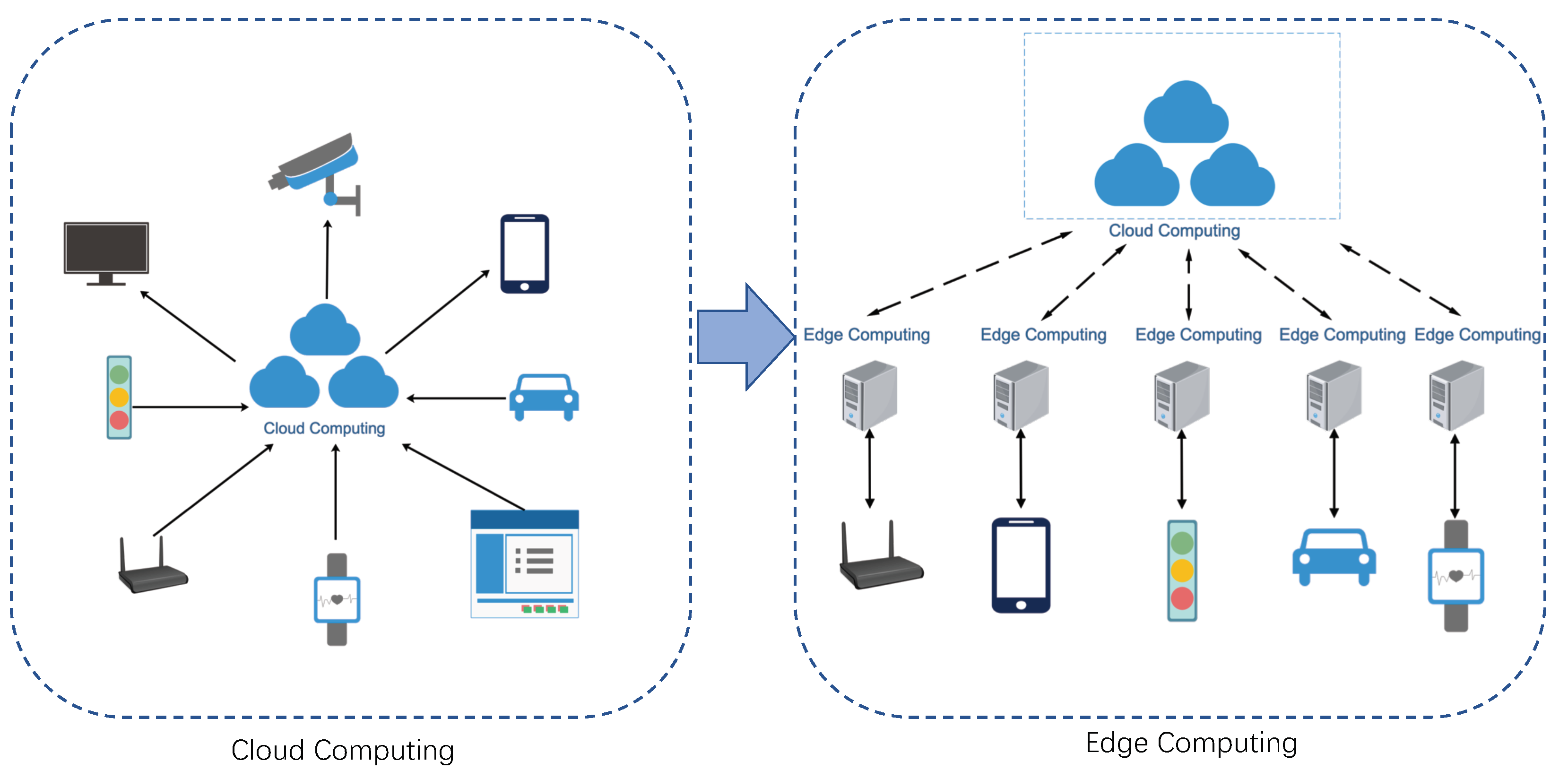
39]. As shown in
Figure 4.
Cloud and Edge Computing
Cloud computing is a paradigm for enabling ubiquitous, convenient, on-demand network access to a shared pool of configurable computing resources (e.g., networks, servers, storage, applications, and services), which can be rapidly provisioned and released with minimal management efforts or service provider interaction.
With cloud computing, edge computing emerges as a novel form of computing paradigm, which shifts from centralized to decentralized [
40]. Compared with conventional cloud computing, it provides shorter response times and better reliability. To save bandwidth and reduce the latency, more data is processed at the edge rather than uploaded to the cloud. Thus, mobile devices of users can complete parts of the workload at the edge of the network. Similarly, in modern transportation, edge devices can be deployed on roadsides and in vehicles for better communications and control between connected objects.
3. Preliminary
3.1. Multi-Agent Communication Model
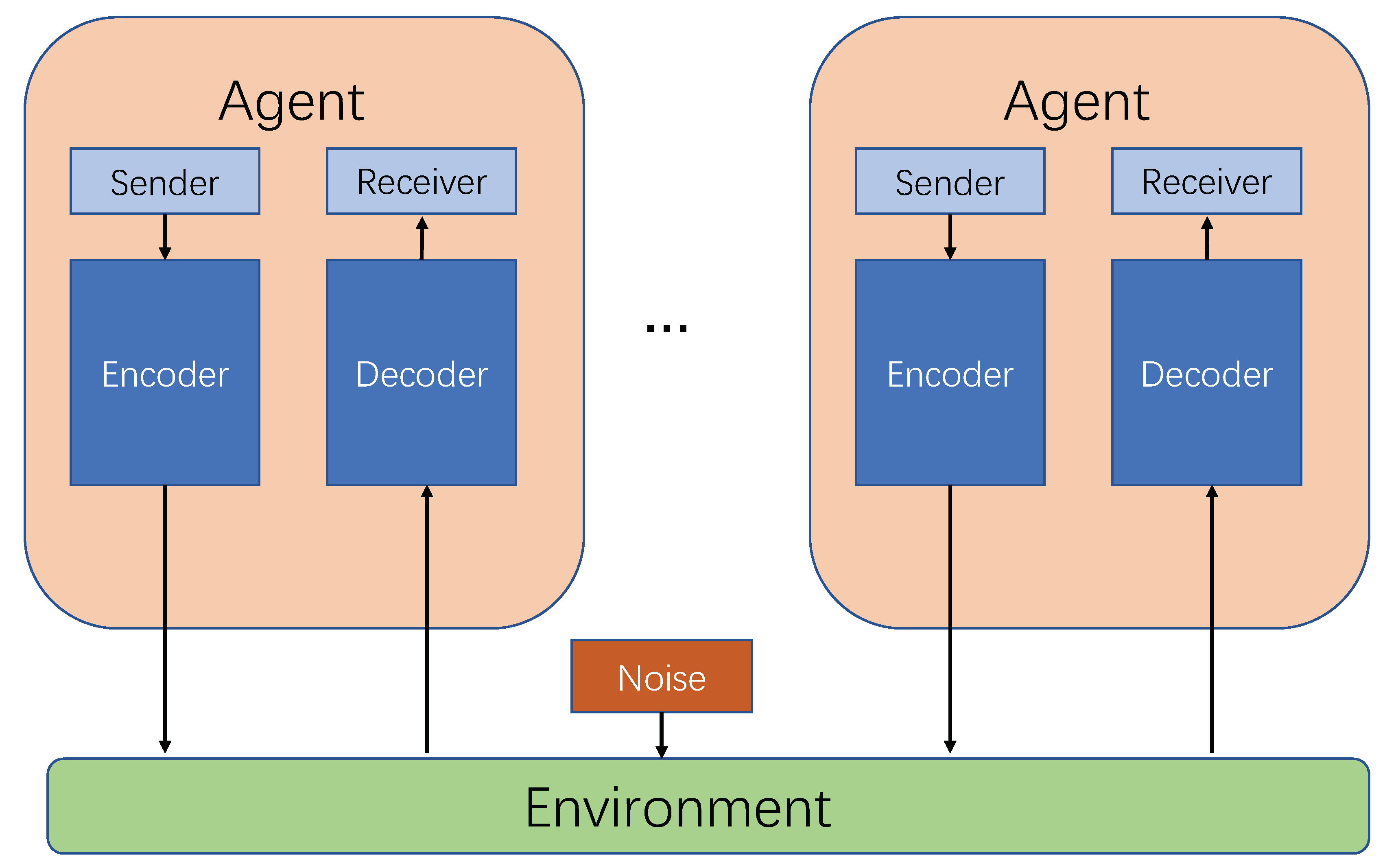
The multi-agent communication model (as shown in
Figure 5) is in accordance with Shannon communication model [
41], the applied perception and behavior of agents can be modeled by information reception and transmission. The agent acts as a communication transceiver, and the internal structure information of the agent is encoded and decoded. The environment is the communication channel between the agents. In actual modeling, a continuous matrix is generally used for multi-agent communication [
18,
42].
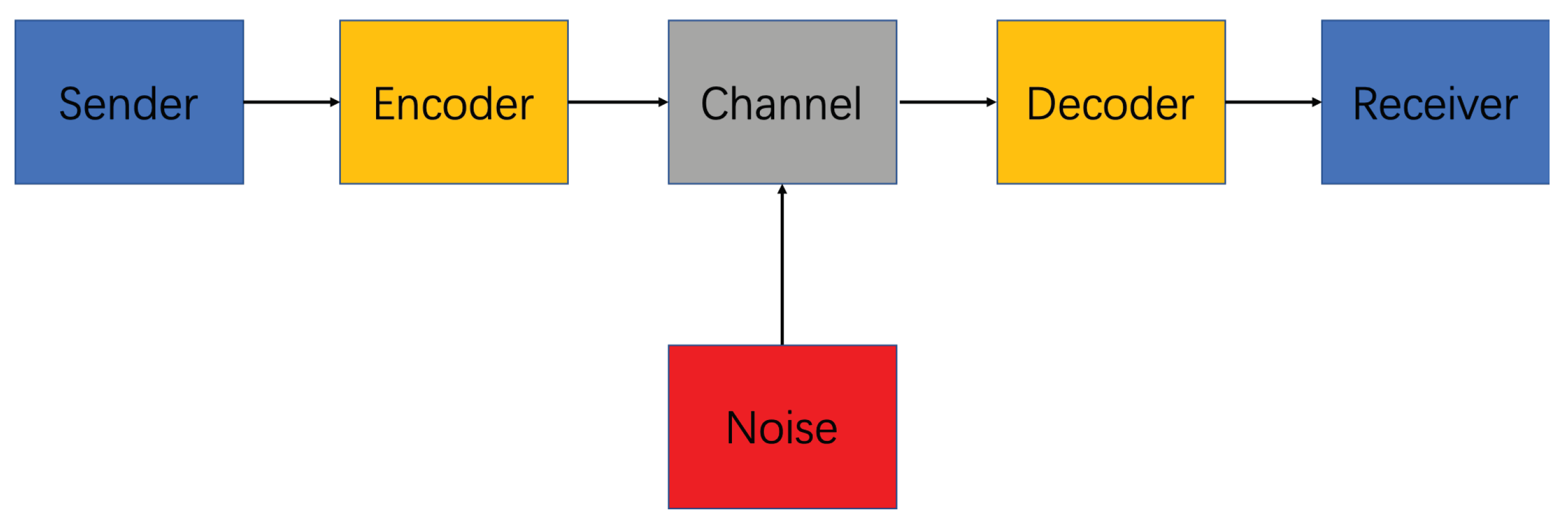
3.1.1. Shannon Communication Model
The basic problem of communication is to reproduce a message sent from one point to another point. In 1948, Shannon proposed the Shannon communication model [
41], which represented the beginning of modern communication theory. Shannon communication model is a linear communication model, consisting of six parts: sender, encoder, channel, noise, decoder, and receiver, as shown in
Figure 6:
3.1.2. Communications Protocol
The communication protocol [
43] is also called the transmission protocol. Both parties involved in the communication carried out end-to-end information transmission according to the agreed rules, and both parties can understand the received information. The communication protocol is mainly composed of grammar, semantics, and timing. The syntax includes the data format, encoding, and signal level; the semantics represent the data content that contains control information, and the timing represents clear rate matching and sequencing of communications.
3.2. Problem Definition
In the problem of multi-agent traffic signal control, we consider it as a Markov Decision Process (MDP):
, where x the state of all intersections;
is the policy to create actions; R is reward from all crossroads;
is the discount factor. Furthermore, we define: each agent that controls the change (duration) of traffic lights is
;
is
for all acceptable traffic light duration control strategies, rewarding the
environment for the level of traffic congestion at the intersection of
and other Agents (
and its policy
) (It can be calculated according to the specific indicators of vehicle queue length, the lower the congestion level, the greater the reward),
is the communication matrix
C between agents, so in our multi-agent traffic signal problem, the objective functions controlled are:
In the Eqution (
4),
is the policy of
;
is the policy of
;
t is the timestep. The problem is to find a better strategy to maximize the value of the above formula.
4. Methodology
In this section, we will detail the multi-agent auto communication (MAAC) model and an edge computing architecture for IoT.
4.1. MAAC Model
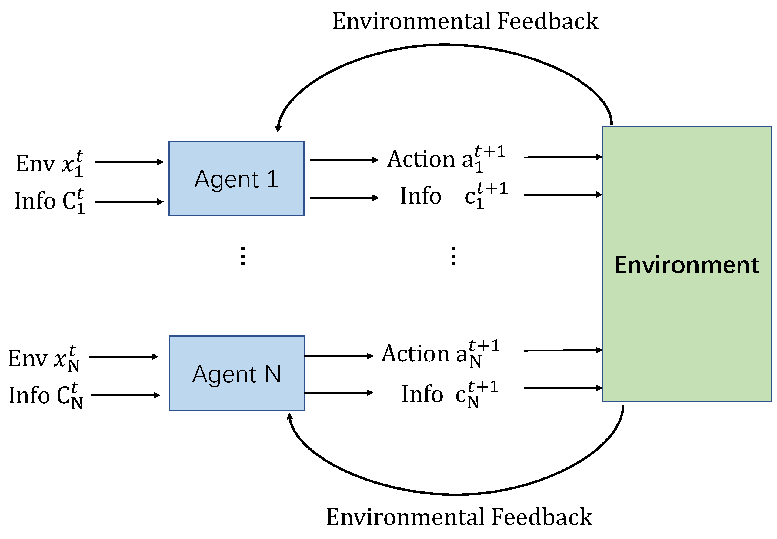
In the MAAC model (as shown in
Figure 7):
Each agent can be modeled by distributed, partially observable Markov decision (Dec-POMDP). The strategy of each agent () is generated by a neural network. In each time step, the agent will observe the local environment and the communication information sent by other agents . Through the combination of the above time series information, the Agent generates the next action and the next communication message sent out by the internal processing mechanism (parameter is ).
The joint actions of all Agents ( ) interact with the environment, which is to obtain the maximum value of the centralized value function . The MAAC algorithm is designed to improve the neural network parameter set of each agent through the process of optimizing the central value function. The overall architecture of the MAAC model can be regarded as a distributed MARL model with automatic communication capabilities.
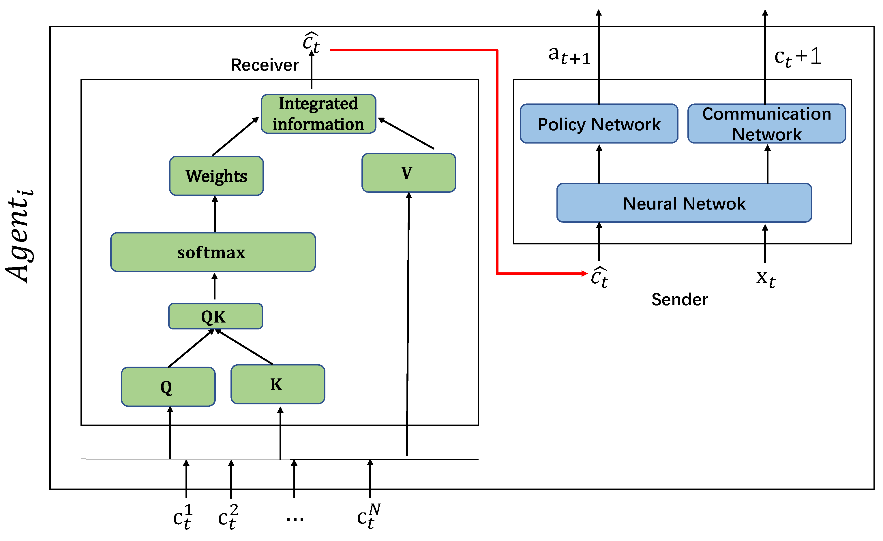
4.1.1. Internal Communication Module in Agent
The internal communication module (ICM) in an agent is an important part in MAAC model (as shown in
Figure 8).
Each Agent, which is divided into two sub-modules, with the receiving end and the sending end. The receiving end receives the information of other agents and uses the attention mechanism for information processing, and then sends the processed information to the sending end; the sending end observes the external environment and uses the information processed by the receiving attention mechanism to generate information using a neural network.
Receiving End
will use the attention mechanism to filter information received from other Agents (
). Firstly it generates its own message
from a combined message
after receiving the information of
. Then, it picks important messages and ignores unimportant ones. Herein, we introduce the parameter set
,
, which are calculated separately (could be calculated in parallel):
Then, we calculate the information weight . Finally we get the weighted information after the information selection: .
Sending End
The sending end of the Agent receives the information of other Agents processed by the Attention mechanism of the receiving end , and through the observed local environment , generates the next execution action through the neural network and communication information .
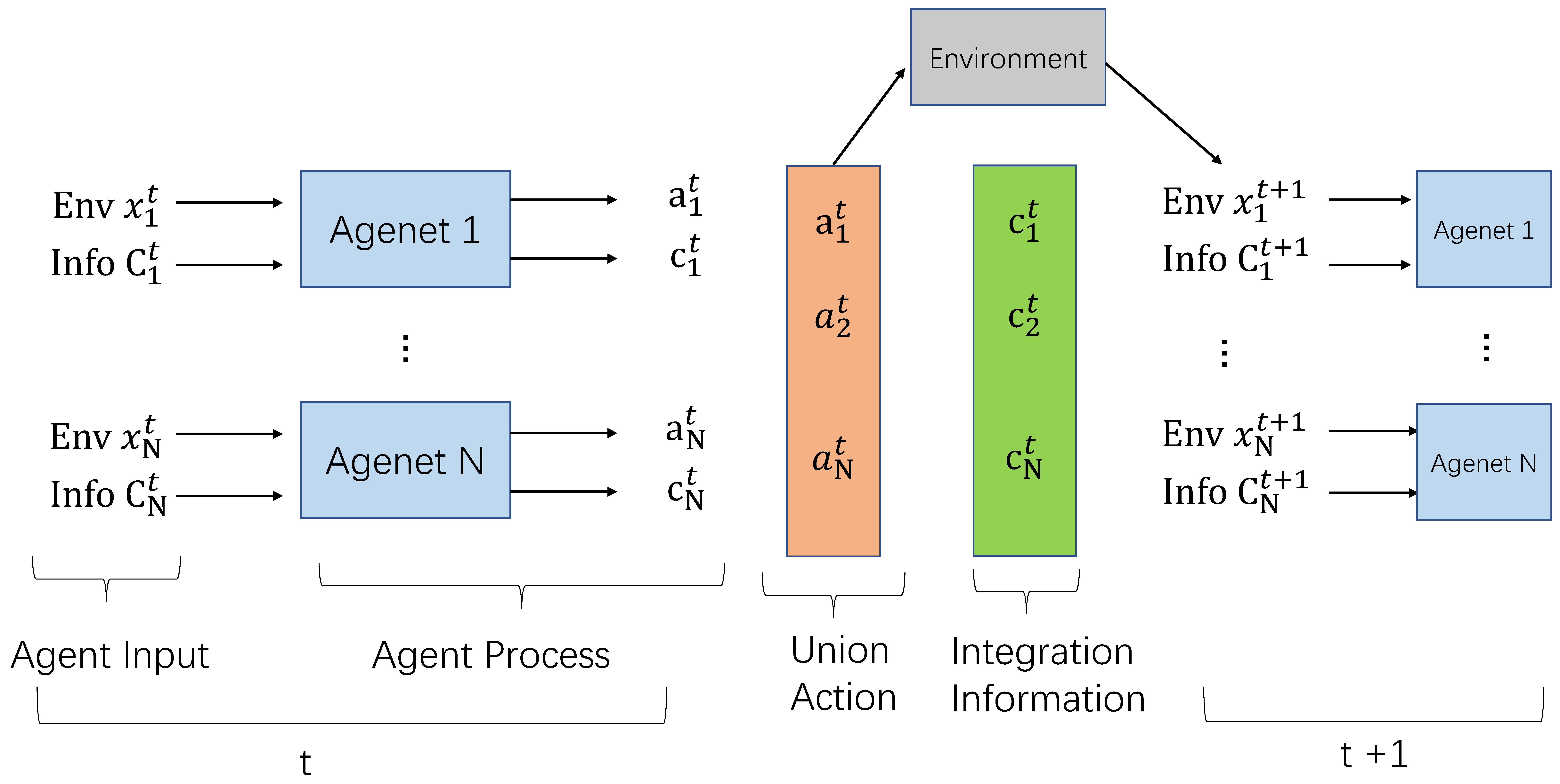
4.1.2. MAAC Algorithm
At the time of
t in the MAAC model, the environment input is
and corresponding communication information input is
. Multi-agents (
) are going to interact with each other. Each Agent receives information with receivers and transmitters internally. The receiver receives its own environmental information
and communication information
, and generates action and external interaction information group
at
. The MAAC model collects all agent actions to form a joint action (
), interacting with the environment and optimizing objective strategy for each agent.
The calculation steps of MAAC at time
t are shown in the
Figure 9:
In the MAAC algorithm (as shown in Algorithm 1), the parameter set of
for each agent is
. Furthermore,
is divided into the sender
and receiver
. The parameters of the sending end and the receiving end, which are optimized by the overall multi-agent objective function, iteratively updating the parameter set of the receiver and the sender in the communication module of each agent.
| Algorithm 1 MAAC learning algorithm process |
| 1: Initialize the communication matrix of all agents |
| 2: Initialize the parameters of the agent and |
| 3: repeat |
| 4: Receiver of : uses attention mechanism to generate communication matrix |
5: Sender of : chooses an action from policy selection network, or randomly chooses
action a (e.g.,-greedy exploration) |
6: Sender of : generates its own information through the receiver’s communication matrix
|
7: Collect all the joint actions of Agent and execute the actions , get the reward from
the environment and next state |
8: Update the strategic value function of each Agent:
|
| 9: until End of Round Episode |
| 10: returns and for each Agent |
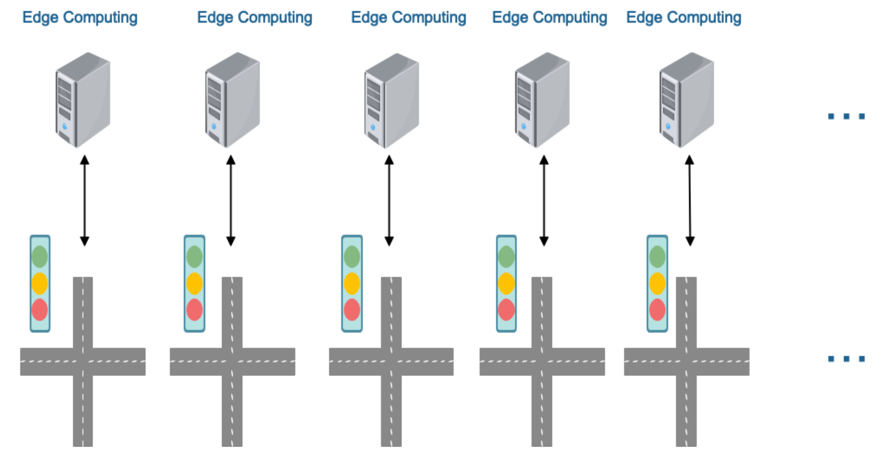
4.2. Edge Computing Structure
In order to deploy MAAC algorithms in an industrial scale environment, we must take the network delay into consideration. We propose an edge computing architecture near every traffic light. An edge computing device needs to have the following functions: (1) it could detect vehicles’ information (location, direction, velocity) from the surveillance video of its intersection in real-time and record the vehicle information; (2) it could run the traffic signal control algorithm to control the traffic light nearby (see
Figure 10).
5. Experiments
In this section, we first built the urban traffic simulator based on our edge computing architecture. Then, we have applied the MAAC algorithm and other baseline algorithms to the simulation environment for comparing the performance of all models.
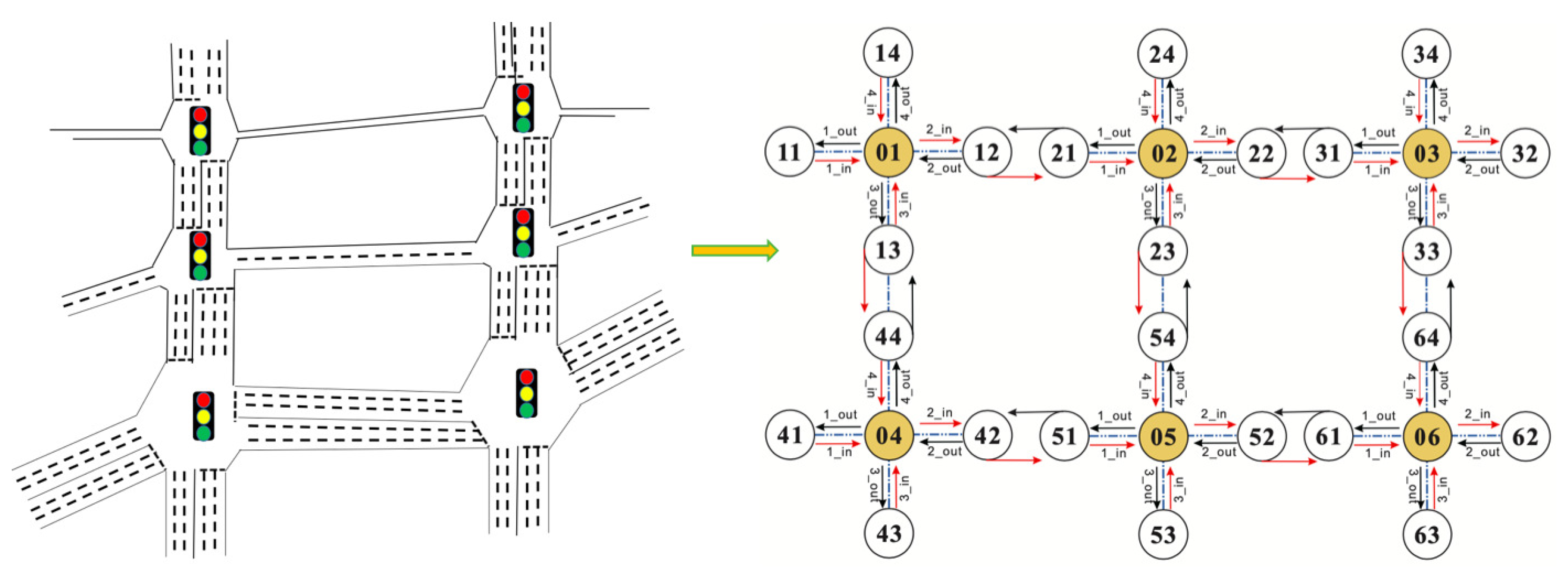
5.1. Simulation Environment and Settings
We apply an open source simulator for traffic environment: CityFlow [
44] as our experiment environment. We assumed that there are six traffic lights (intersection nodes or edge computing nodes) in one section of a city (as shown in
Figure 11).
Our dynamic control of the traffic lights was using the CityFlow [
44] Python interface at runtime.
Here are the settings of our experiments (as shown in
Table 2).
The directions
One traffic light at has four neighbor nodes , four entries (in), and four exits (out). The road length is set to 350 m and vehicle speed limit is set to be 30 (km/h).
Traffic light agent
We apply traffic signal control algorithm into a docker container [
45].
Communication delay setting
The communication delay from center to a traffic light is set as 1 s (sleep 1 s in the code).
Traffic control timing cycle
We initially set a traffic light time cycle as 45 s, and green light interval s, red light interval s, and yellow light interval s.
Episode
One episode time is set as 15 min (900 s), including 20 traffic light time cycles.
Vehicle simulation setting
We assume vehicles arrive at road entrances according to the Bernoulli process with the random probability at one intersection. Every vehicle has a random destination node except for the entry node (we set ). In one episode, there are approximately 400 vehicles.
Hyper-parameter setting
The learning rate is set to 0.001; is set to 0.992; the reward is the average waiting time at intersection.
5.3. Evaluation
The time of a vehicle enters an entry of the intersection until it passes through, is defined as , where M is the number of vehicles. In simulations, we record the time for all vehicles at one intersection in every episode. At last, we accumulate all the times record over all the intersections, . To evaluate the traffic network, where E is the number of the episode, M is the number of vehicles, and I is the number of intersections that every vehicle will pass through.
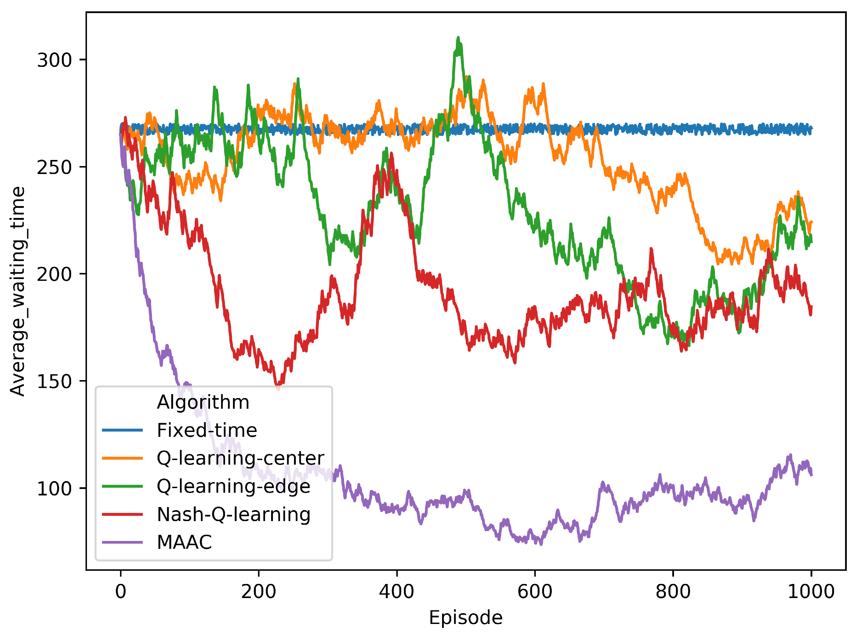
5.4. Results
We have applied five methods, including Fixed-time method [
20], Q-learning (Center) [
46], Q-learning (Edge) [
46], Nash Q-learning [
47], and our MAAC method. They were all trained in 1000 episodes in CityFLow [
44] based on edge computing architecture as we designed. As shown in
Figure 12, we can see that the the algorithms converged at around 600 episode point. The MAAC method performed the fastest convergence in the training process, comparing with other models.
After trainning, we tested the algorithms in 500 episodes after the training process. As shown in
Table 3, the MAAC performed the best among the traffic signal control algorithms.
As shown in
Table 4, our method did not sacrifice the waiting time of some intersections to ensure overall performance. Furthermore, the performance of every intersection was optimized at different levels. From the method Q-learning (center) and Q-learning (edge), we can see that the edge computing structure has reduced the network delay for the deployment environment.
As shown in
Table 5, the delay time and delay rate of Q-learning (Center) are the highest, which proves the edge computing structure we proposed is useful for reducing the network delay. The MAAC still outperforms others when computing the delay time of the network.
6. Conclusions
In this work, we proposed a multi-agent auto communication (MAAC) algorithm based on the multi-agent reinforcement learning (MARL) and an auto communication protocol (ACP) between agents with the attention mechanism. We built a practicable edge computing structure for industrial deployment on IoT, considering the limitations of the capabilities of network transmission bandwidth.
In the simulation environment, the experiments have shown the MAAC framework outperformed 17% over baseline models. Moreover, the edge computing structure is useful for reducing the network delay when deploying the algorithm on an industrial scale.
In future research, we will build a simulation environment much closer to the real world and take the communication from vehicle to traffic light into consideration to improve the MAAC method.
Author Contributions
Conceptualization, Q.W. and J.W.; methodology, Q.W. and J.S.; software, B.Y.; validation, J.S. and Q.Z.; formal analysis, Q.Z. All authors have read and agreed to the published version of the manuscript.
Funding
This research received no external funding.
Acknowledgments
This work was supported by Ministry of Education—China Mobile Research Foundation under Grant No. MCM20170206, The Fundamental Research Funds for the Central Universities under Grant No. lzujbky-2019-kb51 and lzujbky-2018-k12, National Natural Science Foundation of China under Grant No. 61402210, Major National Project of High Resolution Earth Observation System under Grant No. 30-Y20A34-9010-15/17, State Grid Corporation of China Science and Technology Project under Grant No. SGGSKY00WYJS2000062, Program for New Century Excellent Talents in University under Grant No. NCET-12-0250, Strategic Priority Research Program of the Chinese Academy of Sciences with Grant No. XDA03030100, Google Research Awards and Google Faculty Award. We also gratefully acknowledge the support of NVIDIA Corporation with the donation of the Jetson TX1 used for this research. Jianqing Wu also would like to gratefully acknowledge financial support from the China Scholarship Council (201608320168). Jun Shen’s collaboration was supported by University of Wollongong’s University Internationalization Committee Linkage grant and Chinese Ministry of Education’s International Expert Fund “Chunhui Project” awarded to Lanzhou University.
Conflicts of Interest
The authors declare no conflict of interest.
References
- Abdulhai, B.; Pringle, R.; Karakoulas, G.J. Reinforcement learning for true adaptive traffic signal control. J. Transp. Eng. 2003, 129, 278–285. [Google Scholar] [CrossRef] [Green Version]
- Richard, S.S.; Andrew, G.B. Reinforcement Learning: An Introduction. MIT Press 2005, 16, 285–286. [Google Scholar]
- Ghazal, B.; ElKhatib, K.; Chahine, K.; Kherfan, M. Smart traffic light control system. In Proceedings of the 2016 3rd International Conference on Electrical, Electronics, Computer Engineering and their Applications (EECEA), Beirut, Lebanon, 21–23 April 2016; pp. 140–145. [Google Scholar]
- Wei, H.; Zheng, G.; Yao, H.; Li, Z. IntelliLight: A Reinforcement Learning Approach for Intelligent Traffic Light Control; Association for Computing Machinery: New York, NY, USA, 2018; pp. 2496–2505. [Google Scholar]
- Krizhevsky, A.; Sutskever, I.; Hinton, G.E. Imagenet classification with deep convolutional neural networks. In Advances in Neural Information Processing Systems; The MIT Press: Cambridge, MA, USA, 2012; pp. 1097–1105. [Google Scholar]
- Szegedy, C.; Vanhoucke, V.; Ioffe, S.; Shlens, J.; Wojna, Z. Rethinking the inception architecture for computer vision. In Proceedings of the IEEE Conference on Computer Vision and Pattern Recognition, Las Vegas, NV, USA, 26 June–1 July 2016; pp. 2818–2826. [Google Scholar]
- Simonyan, K.; Zisserman, A. Very deep convolutional networks for large-scale image recognition. arXiv 2014, arXiv:1409.1556. [Google Scholar]
- He, K.; Zhang, X.; Ren, S.; Sun, J. Deep residual learning for image recognition. In Proceedings of the IEEE Conference on Computer Vision and Pattern Recognition, Las Vegas, NV, USA, 26 June–1 July 2016; pp. 770–778. [Google Scholar]
- Hinton, G.; Deng, L.; Yu, D.; Dahl, G.E.; Mohamed, A.R.; Jaitly, N.; Senior, N.; Vanhoucke, V.; Nguyen, P.; Sainath, T.N.; et al. Deep neural networks for acoustic modeling in speech recognition. IEEE Signal Process. Mag. 2012, 29, 82–97. [Google Scholar] [CrossRef]
- Bahdanau, D.; Cho, K.; Bengio, Y. Neural machine translation by jointly learning to align and translate. arXiv 2014, arXiv:1409.0473. [Google Scholar]
- Kingma, D.P.; Ba, J. Adam: A method for stochastic optimization. arXiv 2014, arXiv:1412.6980. [Google Scholar]
- Vaswani, A.; Shazeer, N.; Parmar, N.; Uszkoreit, J.; Jones, L.; Gomez, A.N. Attention is All you Need. In Proceedings of the 31st International Conference on Neural Information Processing Systems, Long Beach, CA, USA, 4–9 December 2017. [Google Scholar]
- Zhou, R.; Li, X.; Yong, B.; Shen, Z.; Wang, C.; Zhou, Q.; Li, K.C. Arrhythmia recognition and classification through deep learning-based approach. Int. J. Comput. Sci. Eng. 2019, 19, 506–517. [Google Scholar] [CrossRef]
- Wu, Q.; Shen, J.; Yong, B.; Wu, J.; Li, F.; Wang, J.; Zhou, Q. Smart fog based workflow for traffic control networks. Future Gener. Comput. Syst. 2019, 97, 825–835. [Google Scholar] [CrossRef]
- Yong, B.; Xu, Z.; Shen, J.; Chen, H.; Wu, J.; Li, F.; Zhou, Q. A novel Monte Carlo-based neural network model for electricity load forecasting. Int. J. Embed. Syst. 2020, 12, 522–533. [Google Scholar] [CrossRef]
- Silver, D.; Schrittwieser, J.; Simonyan, K.; Antonoglou, I.; Huang, A.; Guez, A.; Hubert, T.; Baker, L.; Lai, M.; Bolton, A.; et al. Mastering the game of go without human knowledge. Nature 2017, 550, 354. [Google Scholar] [CrossRef]
- Bazzan, A.L. Opportunities for multi-agent systems and multi-agent reinforcement learning in traffic control. Auton. Agents Multi-Agent Syst. 2009, 18, 342. [Google Scholar] [CrossRef]
- Sukhbaatar, S.; Fergus, R. Learning multiagent communication with backpropagation. NIPS 2016, 2244–2252. [Google Scholar]
- Hoshen, Y. Attentional multi-agent predictive modeling. Neural Inf. Process. Syst. (NIPS) 2017, 2701–2711. [Google Scholar]
- Webster, F. Traffic signal settings. H.M. Station. Off. 1958, 39, 45. [Google Scholar]
- Thorpe, T.L. Vehicle Traffic Light Control Using SARSA; Colorado State University: Fort Collins, CO, USA, 1997. [Google Scholar]
- Chiou, S.W. An efficient algorithm for computing traffic equilibria using TRANSYT model. Appl. Math. Model. 2010, 34, 3390–3399. [Google Scholar] [CrossRef]
- Chaib-Draa, B.; Moulin, B.; Millot, P. Trends in distributed artificial intelligence. Artif. Intell. Rev. 1992, 6, 35–66. [Google Scholar] [CrossRef]
- Durfee, E.H.; Lesser, V.R. Negotiating task decomposition and allocation using partial global planning. Distrib. Artif. Intell. 1989, 2, 229–243. [Google Scholar]
- Minsky, M. The Emotion Machine: Commonsense Thinking, Artificial Intelligence, and the Future of the Human Mind; Simon & Schuster: New York, NY, USA, 2007. [Google Scholar]
- Peng, P.; Yuan, Q.; Wen, Y.; Yang, Y.; Tang, Z.; Long, H.; Wang, J. Multiagent Bidirectionally-Coordinated Nets for Learning to Play StarCraft Combat Games. arXiv 2017, arXiv:1703.10069. [Google Scholar]
- Chen, C.; Wei, H.; Xu, N.; Zheng, G.; Yang, M.; Xiong, Y.; Xu, K.; Li, Z. Toward a Thousand Lights: Decentralized Deep Reinforcement Learning for Large-Scale Traffic Signal Control. AAAI 2020, 34, 3414–3421. [Google Scholar] [CrossRef]
- Prashanth, L.A.; Bhatnagar, S. Reinforcement learning with function approximation for traffic signal control. IEEE Trans. Intell. Transp. Syst. 2010, 12, 412–421. [Google Scholar]
- Mousavi, S.S.; Schukat, M.; Howley, E. Traffic light control using deep policy-gradient and value-function-based reinforcement learning. IET Intell. Transp. Syst. 2017, 11, 417–423. [Google Scholar] [CrossRef] [Green Version]
- El, -T.S.; Abdulhai, B. Towards multi-agent reinforcement learning for integrated network of optimal traffic controllers (MARLIN-OTC). Transp. Lett. 2010, 2, 89–110. [Google Scholar] [CrossRef]
- Weinberg, M.; Rosenschein, J.S. Best-response multiagent learning in non-stationary environments. In Proceedings of the 3rd International Joint Conference on Autonomous Agents and Multiagent Systems, New York, NY, USA, 19–23 August 2004. [Google Scholar]
- Xu, K.; Ba, J.; Kiros, R.; Cho, K.; Courville, A.; Salakhudinov, R.; Zemel, R.S.; Bengio, Y. Show, Attend and Tell: Neural Image Caption Generation with Visual Attention. Comput. Sci. 2015, 37, 2048–2057. [Google Scholar]
- Luong, M.T.; Pham, H.; Manning, C.D. Effective Approaches to Attention-based Neural Machine Translation. arXiv 2015, arXiv:1508.04025. [Google Scholar]
- Pottie, G.J. Wireless sensor networks. In Proceedings of the 1998 Information Theory Workshop (Cat. No.98EX131), Killarney, Ireland, 22–26 June 1998; pp. 139–140. [Google Scholar] [CrossRef] [Green Version]
- Jell, A.; Vogel, T.; Ostler, D.; Marahrens, N.; Wilhelm, D.; Samm, N.; Eichinger, J.; Weigel, W.; Feussner, H.; Friess, H.; et al. 5th-Generation Mobile Communication: Data Highway for Surgery 4.0. Surg. Technol. Int. 2019, 35, 36–42. [Google Scholar]
- Atzori, L.; Iera, A.; Morabito, G. The internet of things: A survey. Inf. Syst. Front. 2015, 17, 243–259. [Google Scholar]
- de C. Neto, J.M.; Neto, S.F.G.; M. de Santana, P.; de Sousa, V.A., Jr. Multi-Cell LTE-U/Wi-Fi Coexistence Evaluation Using a Reinforcement Learning Framework. Sensors 2020, 20, 1855. [Google Scholar]
- Faheem, M.; Butt, R.A.; Raza, B.; Alquhayz, H.; Ashraf, M.W.; Shah, S.B.; Ngadi, M.A.; Gungor, V.C. A Cross-Layer QoS Channel-Aware Routing Protocol for the Internet of Underwater Acoustic Sensor Networks. Sensors 2019, 19, 4762. [Google Scholar] [CrossRef] [Green Version]
- Zikria, Y.B.; Afzal, M.K.; Kim, S.W. Internet of Multimedia Things (IoMT): Opportunities, Challenges and Solution. Sensors 2020, 20, 2334. [Google Scholar] [CrossRef]
- Yong, B.; Xu, Z.; Wang, X.; Cheng, L.; Li, X.; Wu, X.; Zhou, Q. IoT-based intelligent fitness system. J. Parallel Distrib. Comput. 2017, 8, 279–292. [Google Scholar]
- Shannon, C.E. A Mathematical Theory of Communication. Bell Syst. Tech. J. 1963, 27, 379–423. [Google Scholar] [CrossRef] [Green Version]
- Foerster, A. Learning to communicate with deep multi-agent reinforcement learning. NIPS 2016, 2145–2153. [Google Scholar]
- West, C.H. General Technique for Communications Protocol Validation. IBM J. Res. Dev. 1978, 22, 393–404. [Google Scholar] [CrossRef]
- Wei, H.; Chen, C.; Zheng, G.; Wu, K.; Xu, K.; Gayah, V.; Li, Z. Presslight: Learning max pressure control for signalized intersections in arterial network. Int. Conf. Knowl. Discov. Data Min. (KDD) 2019, 1290–1298. [Google Scholar] [CrossRef]
- Boettiger, C. An introduction to Docker for reproducible research. ACM SIGOPS Oper. Syst. Rev. 2015, 49, 71–79. [Google Scholar] [CrossRef]
- Watkins, C.J.C.H.; Dayan, P. Q-learning. Mach. Learn. 1992, 8, 279–292. [Google Scholar] [CrossRef]
- Hu, J.W. Nash q-learning for general-sum stochastic games. J. Mach. Learn. Res. 2004, 4, 1039–1069. [Google Scholar]
© 2020 by the authors. Licensee MDPI, Basel, Switzerland. This article is an open access article distributed under the terms and conditions of the Creative Commons Attribution (CC BY) license (http://creativecommons.org/licenses/by/4.0/).


