Figure 1.
Problems with lidar detection using frustums [
29]. Left: Object detected using RGB camera. Right: Detection results in frustum images. Bottom: Obstacles to be removed from frustum image: background (tree) and front obstacle (ground) in the picture.
Figure 1.
Problems with lidar detection using frustums [
29]. Left: Object detected using RGB camera. Right: Detection results in frustum images. Bottom: Obstacles to be removed from frustum image: background (tree) and front obstacle (ground) in the picture.
Figure 2.
Estimated position of the forward vehicle with a lidar sensor.
Figure 2.
Estimated position of the forward vehicle with a lidar sensor.
Figure 3.
Changes in the frustum image according to the distance of the target vehicle: (a) close and (b) far.
Figure 3.
Changes in the frustum image according to the distance of the target vehicle: (a) close and (b) far.
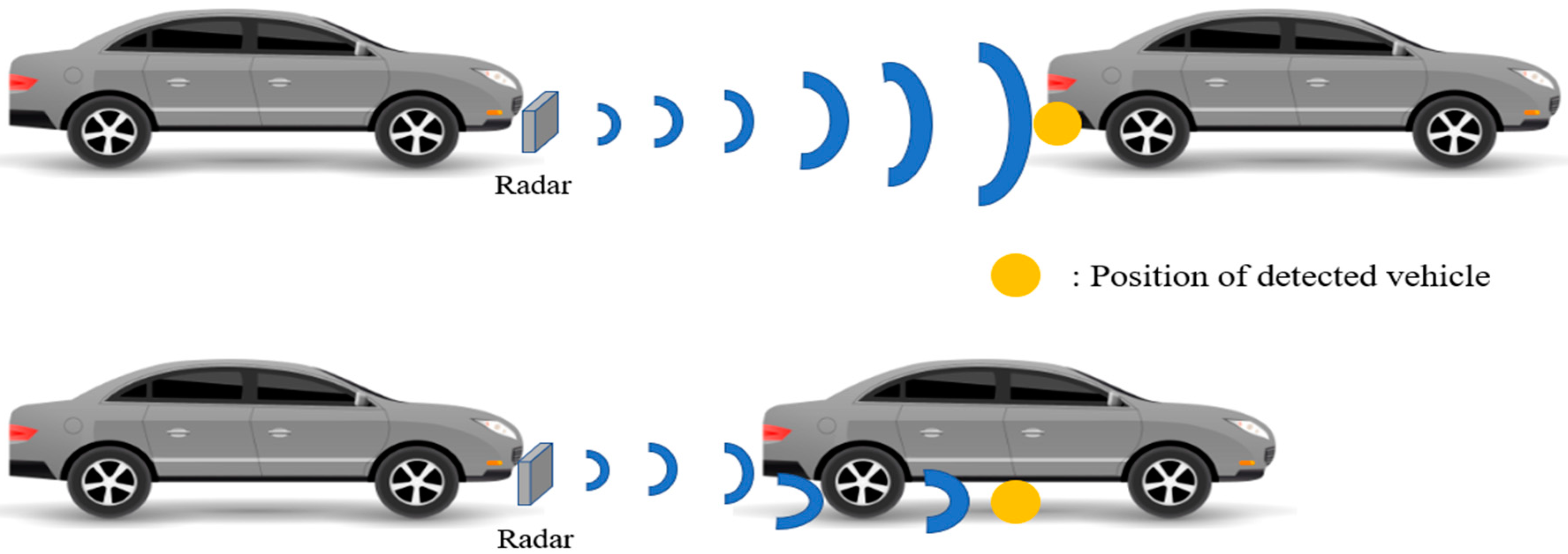
Figure 4.
Problem in measurement values with the radar sensor.
Figure 4.
Problem in measurement values with the radar sensor.
Figure 5.
Measurement error lidar sensor and radar sensor according to distance.
Figure 5.
Measurement error lidar sensor and radar sensor according to distance.
Figure 6.
System structure.
Figure 6.
System structure.
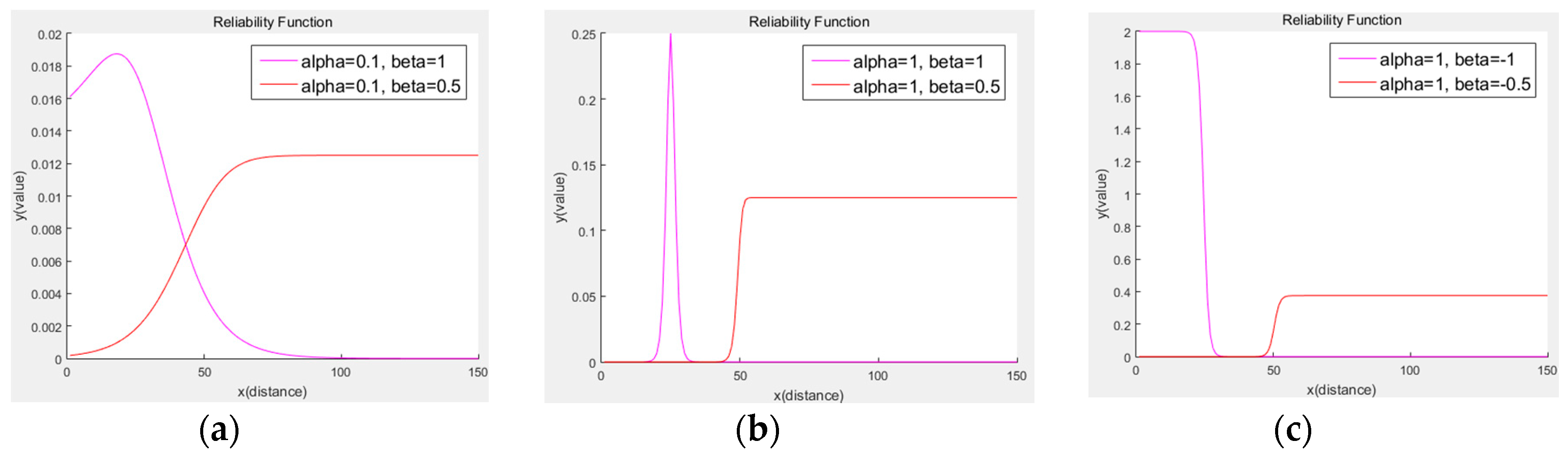
Figure 7.
Reliability function; the x-axis is the distance of the opponent vehicle from the ego vehicle. The y-axis represents the reliability of the value measured by the sensor. When comparing the two sensors, the lidar was accurate at close range, and the radar was accurate at long distances.
Figure 7.
Reliability function; the x-axis is the distance of the opponent vehicle from the ego vehicle. The y-axis represents the reliability of the value measured by the sensor. When comparing the two sensors, the lidar was accurate at close range, and the radar was accurate at long distances.
Figure 8.
Differentiated reliability function; the x-axis is the distance of the opponent vehicle from the ego vehicle. The y-axis represents the reliability of the value.
Figure 8.
Differentiated reliability function; the x-axis is the distance of the opponent vehicle from the ego vehicle. The y-axis represents the reliability of the value.
Figure 9.
Differentiation result of the reliability function according to parameter change: when , (a) = 0.1, = 1 and = 0.1, = 0.5; (b) = 1, = 1 and = 1, = 0.5; (c) = 1, = −1 and = 1, = −0.5.
Figure 9.
Differentiation result of the reliability function according to parameter change: when , (a) = 0.1, = 1 and = 0.1, = 0.5; (b) = 1, = 1 and = 1, = 0.5; (c) = 1, = −1 and = 1, = −0.5.
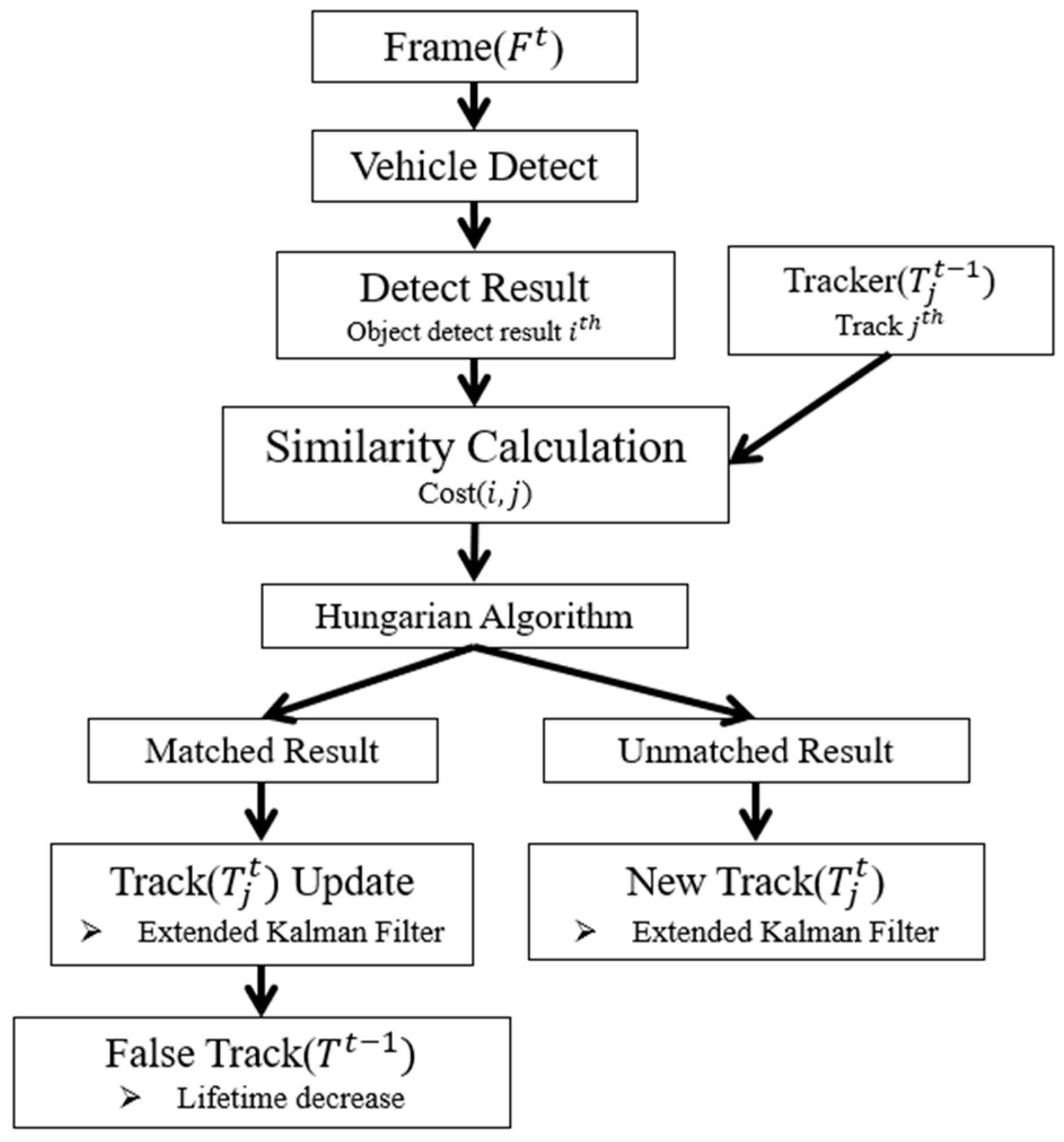
Figure 10.
Tracking management.
Figure 10.
Tracking management.
Figure 11.
Test vehicle. It was equipped with three lidars and one radar.
Figure 11.
Test vehicle. It was equipped with three lidars and one radar.
Figure 12.
Membership function: (a) lidar membership function; (b) radar membership function; (c) output membership function.
Figure 12.
Membership function: (a) lidar membership function; (b) radar membership function; (c) output membership function.
Figure 13.
Test vehicle equipped with three lidars, one radar, and a dashboard camera.
Figure 13.
Test vehicle equipped with three lidars, one radar, and a dashboard camera.
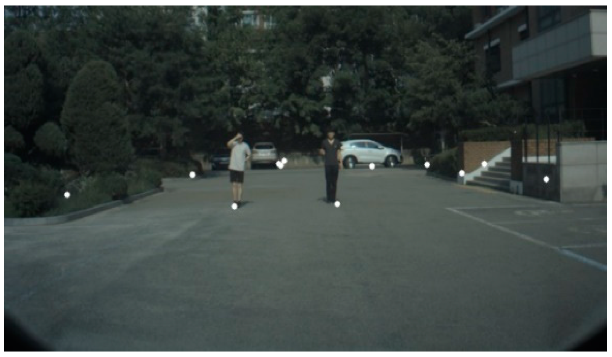
Figure 14.
The result of projecting the radar detection result in the image coordinate system.
Figure 14.
The result of projecting the radar detection result in the image coordinate system.
Figure 15.
Comparison experiment result of other sensor fusion methods: (a) proposed method; (b) adaptive measure noise and Kalman filter; (c) fuzzy method and Kalman filter.
Figure 15.
Comparison experiment result of other sensor fusion methods: (a) proposed method; (b) adaptive measure noise and Kalman filter; (c) fuzzy method and Kalman filter.
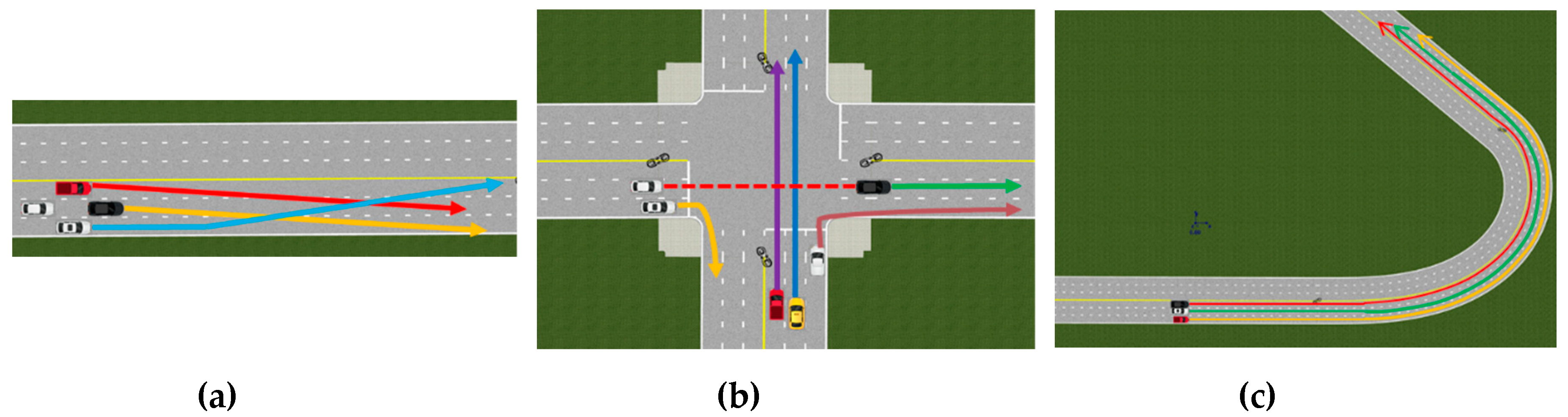
Figure 16.
Simulation of three scenarios: (a) vehicles changing lanes; (b) intersection scenario; (c) curve scenario.
Figure 16.
Simulation of three scenarios: (a) vehicles changing lanes; (b) intersection scenario; (c) curve scenario.
Table 1.
Noise covariances of the proposed algorithm.
Table 1.
Noise covariances of the proposed algorithm.
| Q (Process model noise) | EKF (Proposed) Fuzzy Adaptive | diag (0.5, 0.05, 0.05, 0.05) |
| R (Measurement noise) | EKF (Proposed) | diag (0.05, 0.05, 0.05, 0.05, 0.05) |
| Fuzzy | diag (0.05, 0.05, 0.05) |
| Adaptive | diag (0.05, 0.05, 0.05) |
Table 2.
Fuzzy rules.
| Input | Output |
|---|
| Lidar | Radar | Output Weight |
|---|
| Close | Close | Lidar |
| Middle | Lidar |
| Far | Both |
| Middle | Close | Lidar |
| Middle | Both |
| Far | Radar |
| Far | Close | Both |
| Middle | Radar |
| Far | Radar |
Table 3.
Comparison of the results of the proposed method with other sensor fusion methods.
Table 3.
Comparison of the results of the proposed method with other sensor fusion methods.
| Method RMSE (Frame) | Proposed Method | Adaptive Measure Noise | Fuzzy |
|---|
| Lidar/Radar/Camera | Lidar/Radar/Camera | Lidar/Radar/Camera |
|---|
| x (m) | y (m) | x (m) | y (m) | x (m) | y (m) |
|---|
| Far (681) | 0.29 | 0.30 | 0.41 | 0.38 | 0.28 | 0.34 |
| Close (547) | 0.32 | 0.22 | 0.33 | 0.22 | 0.32 | 0.29 |
| Left turn (152) | 0.55 | 0.35 | 0.54 | 0.36 | 0.61 | 0.33 |
| Right turn (210) | 0.87 | 0.31 | 0.91 | 0.31 | 1.07 | 0.31 |
| Left curve (210) | 0.28 | 0.20 | 0.41 | 0.24 | 0.46 | 0.25 |
| Right curve (72) | 0.39 | 0.25 | 0.47 | 0.30 | 0.25 | 0.22 |
| Total (1882) | 0.38 | 0.27 | 0.50 | 0.33 | 0.40 | 0.30 |
Table 4.
Comparison of the results of the proposed method with fuzzy method in Scenario 1.
Table 4.
Comparison of the results of the proposed method with fuzzy method in Scenario 1.
| Method MOTP (Frame) | Proposed Method | Fuzzy Method |
|---|
| Lidar/Radar/Camera | Lidar/Radar/Camera |
|---|
| x (m) | y (m) | x (m) | y (m) |
|---|
| Vehicle 1 (112) | 1.12 | 1.04 | 1.19 | 1.02 |
| Vehicle 2 (65) | 1.08 | 0.63 | 1.25 | 0.68 |
| Vehicle 3 (128) | 0.93 | 0.67 | 1.04 | 0.66 |
| Total | 1.01 | 0.65 | 1.20 | 0.67 |
Table 5.
Comparison of the results of the proposed method with fuzzy method in Scenario 2.
Table 5.
Comparison of the results of the proposed method with fuzzy method in Scenario 2.
| Method MOTP (Frame) | Proposed Method | Fuzzy Method |
|---|
| Lidar/Radar/Camera | Lidar/Radar/Camera |
|---|
| x (m) | y (m) | x (m) | y (m) |
|---|
| Vehicle 1 (60) | 1.07 | 0.64 | 1.36 | 0.67 |
| Vehicle 2 (67) | 1.12 | 0.91 | 1.17 | 0.89 |
| Vehicle 3 (40) | 1.07 | 0.53 | 1.27 | 0.51 |
| Total | 1.09 | 0.72 | 1.26 | 0.72 |
Table 6.
Comparison of the results of the proposed method with fuzzy method in Scenario 3.
Table 6.
Comparison of the results of the proposed method with fuzzy method in Scenario 3.
| Method MOTP (Frame) | Proposed Method | Fuzzy Method |
|---|
| Lidar/Radar/Camera | Lidar/Radar/Camera |
|---|
| x (m) | y (m) | x (m) | y (m) |
|---|
| Vehicle 1 (155) | 1.12 | 0.35 | 1.42 | 0.32 |
| Vehicle 2 (137) | 0.93 | 0.33 | 1.20 | 0.31 |
| Total | 1.03 | 0.72 | 1.32 | 0.72 |
Table 7.
Comparison of the results of the proposed method with fuzzy method in all scenarios.
Table 7.
Comparison of the results of the proposed method with fuzzy method in all scenarios.
| Method MOTP (Frame) | Proposed Method | Fuzzy Method |
|---|
| Lidar/Radar/Camera | Lidar/Radar/Camera |
|---|
| x (m) | y (m) | x (m) | y (m) |
|---|
| Total | 1.04 | 0.69 | 1.26 | 0.70 |


