Quantitative 3D Reconstruction from Scanning Electron Microscope Images Based on Affine Camera Models

Abstract
:1. Introduction
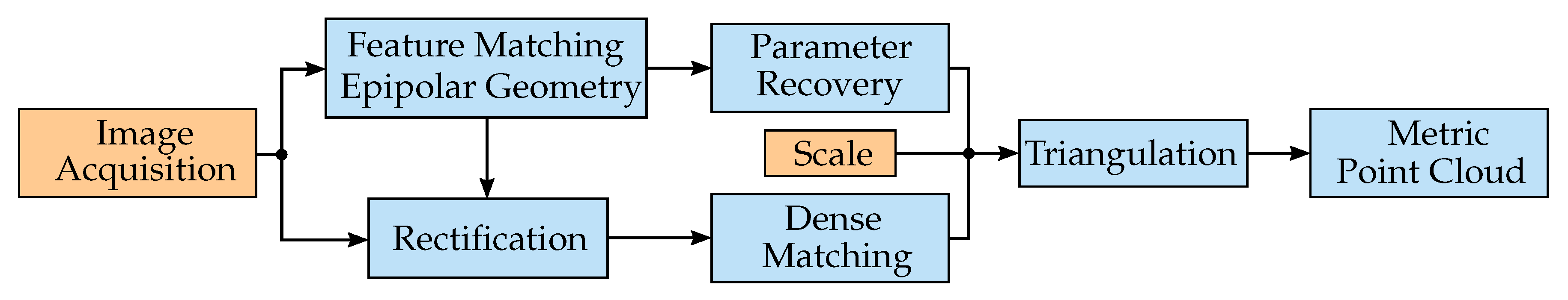
2. Methods
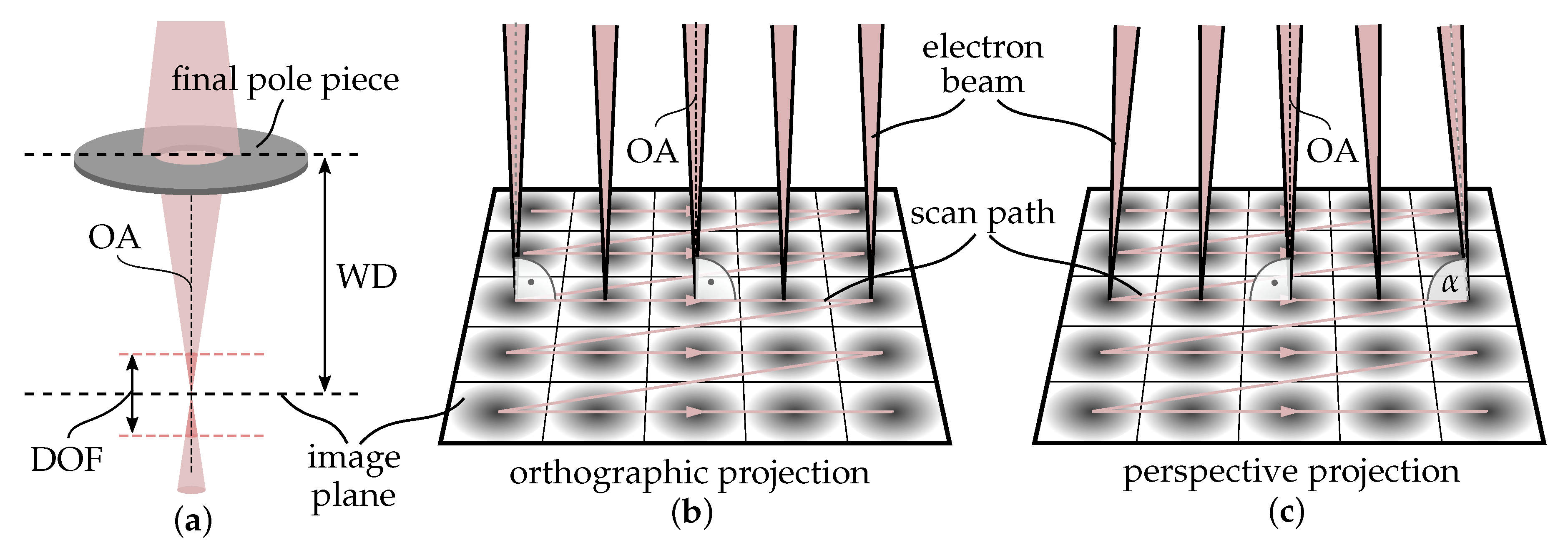
2.1. Affine Camera Model
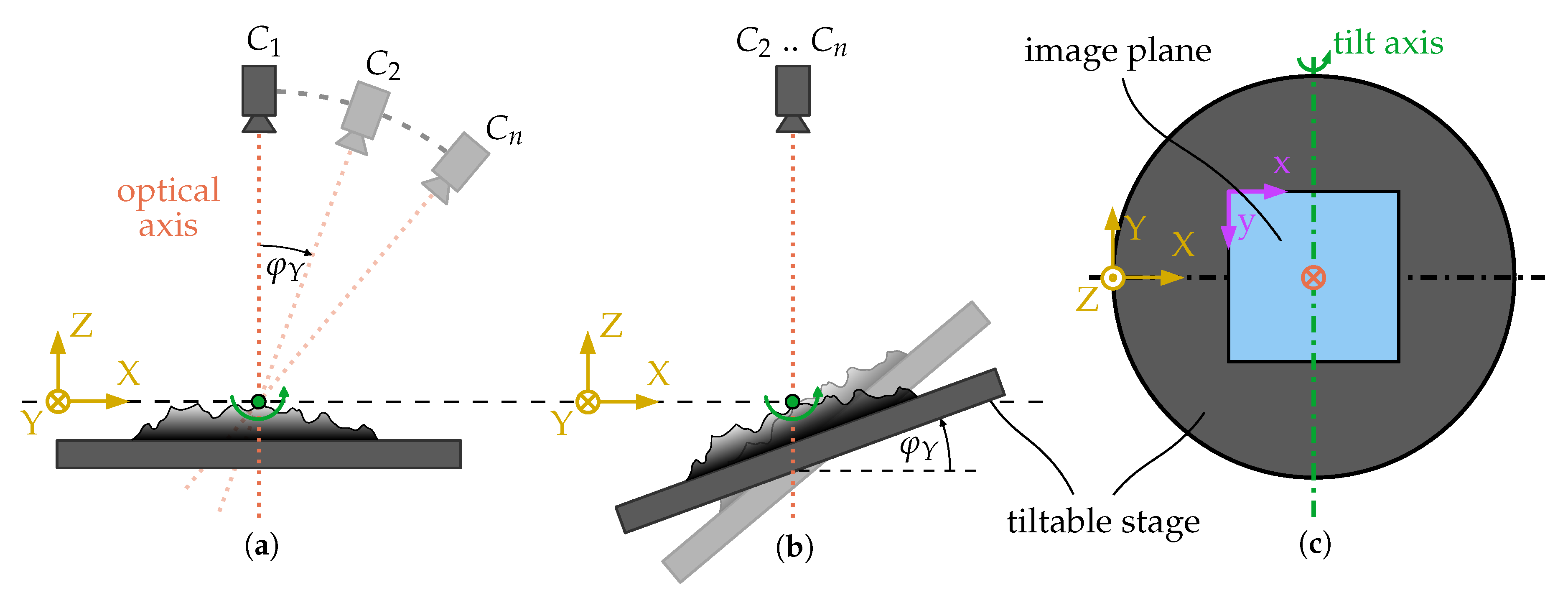
2.2. Stereo Image Acquisition
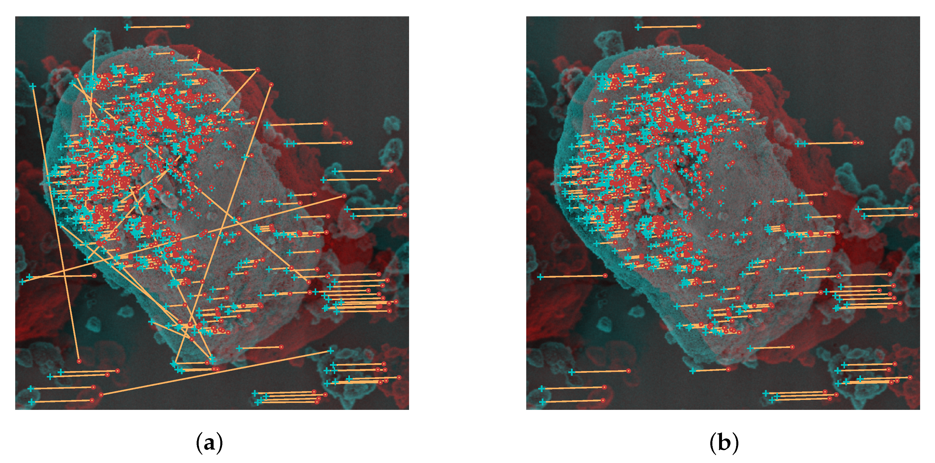
2.3. Feature Matching and Epipolar Geometry
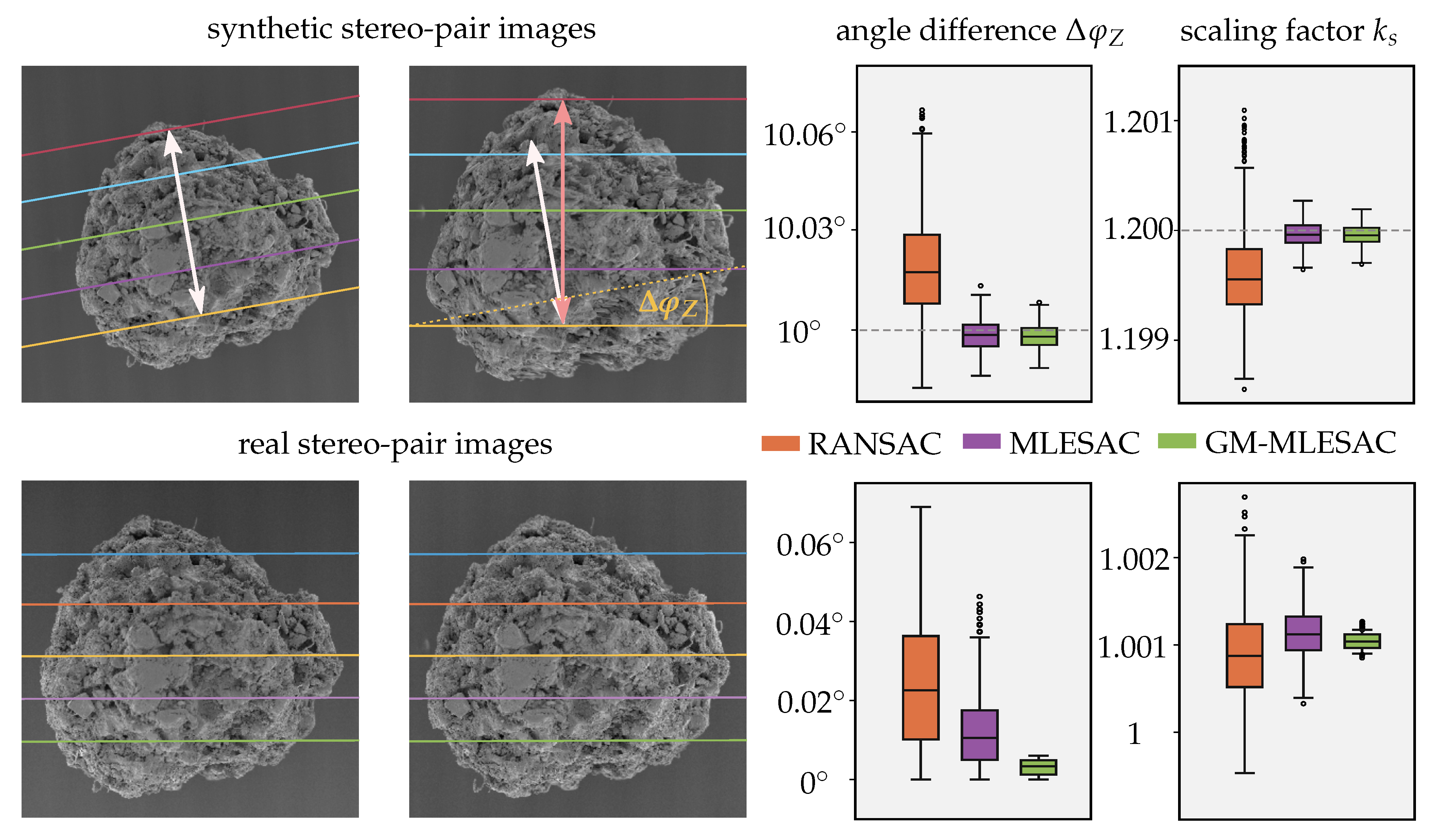
2.4. Parameter Recovery
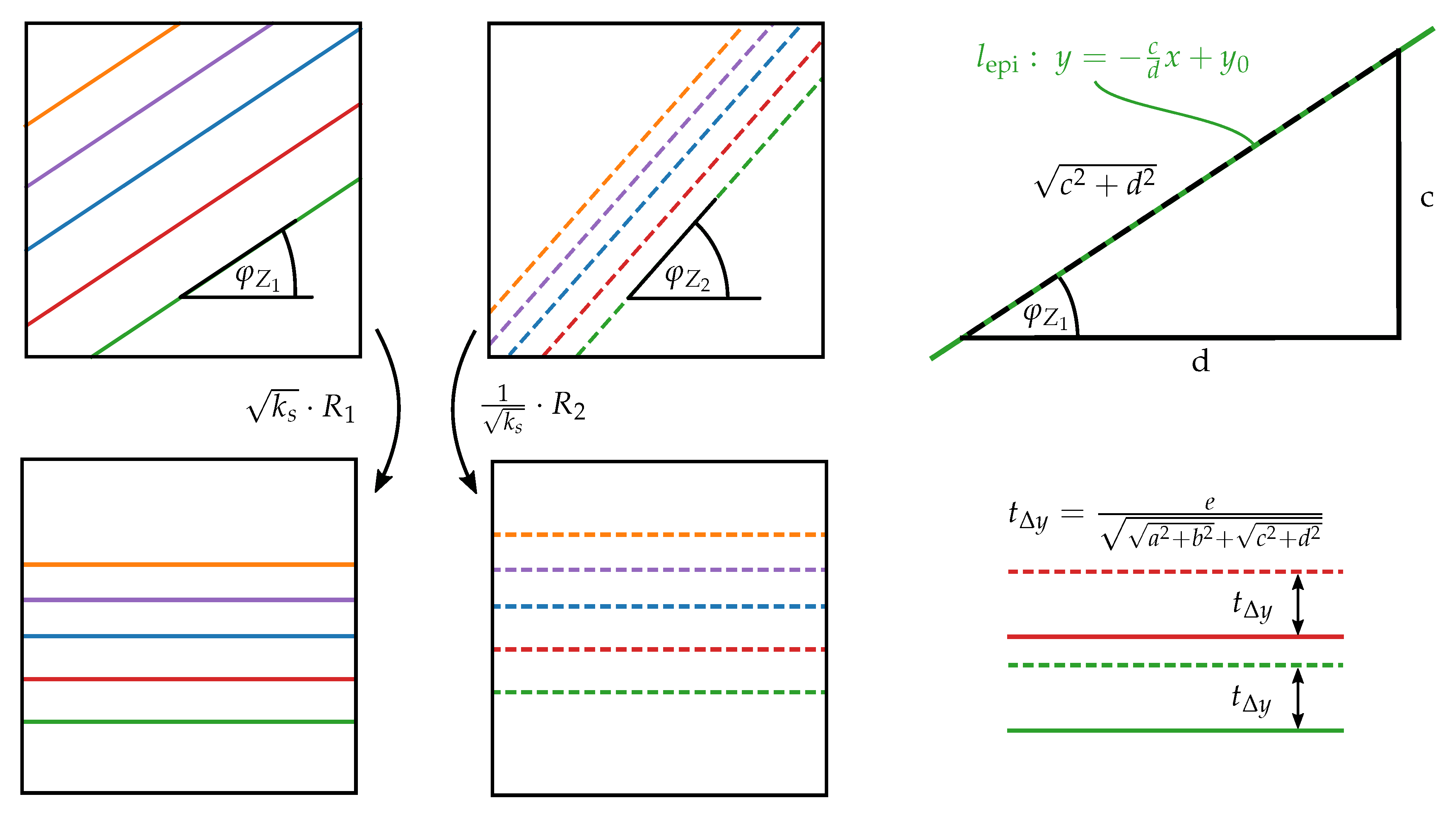
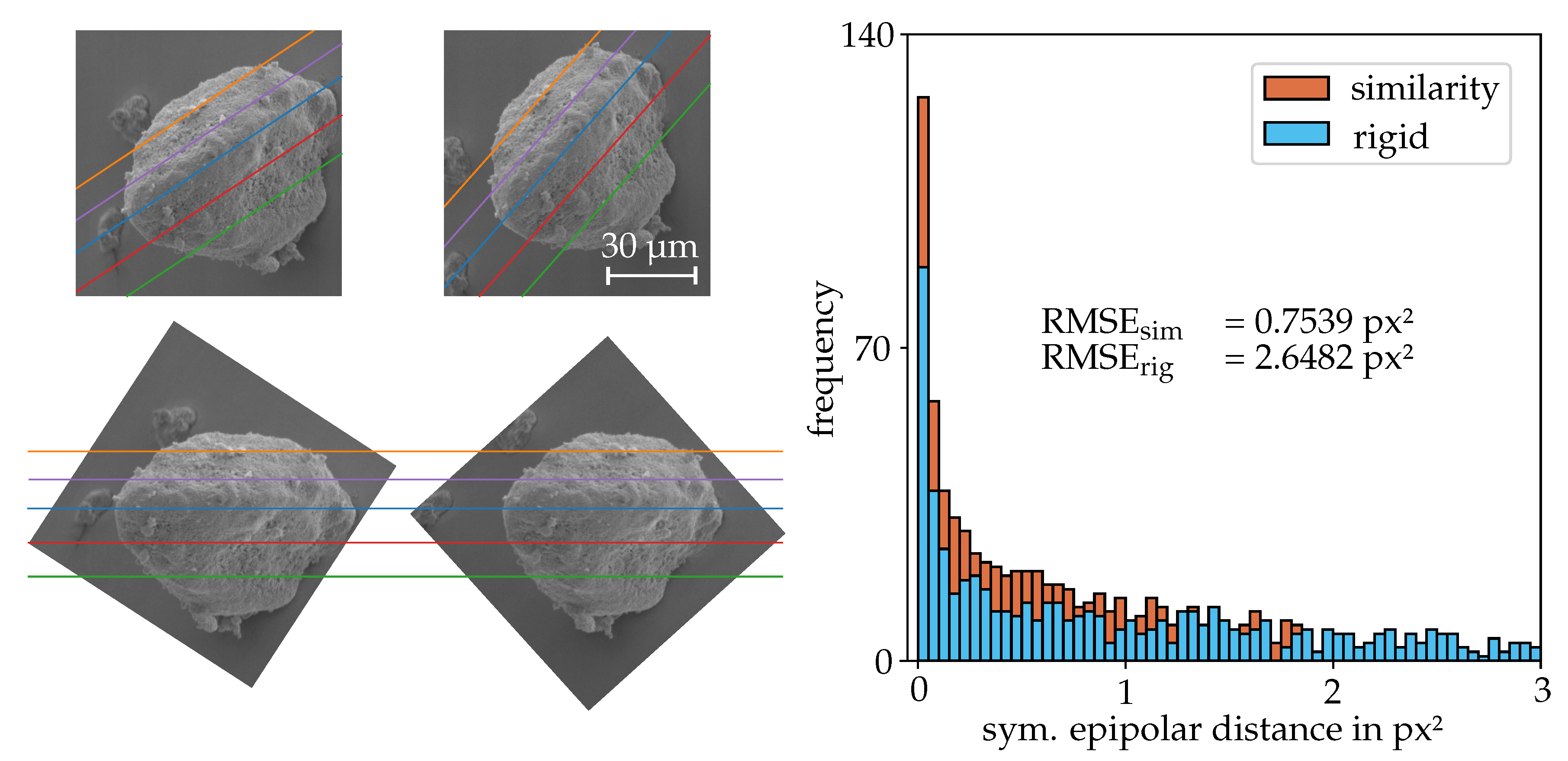
2.5. Rectification
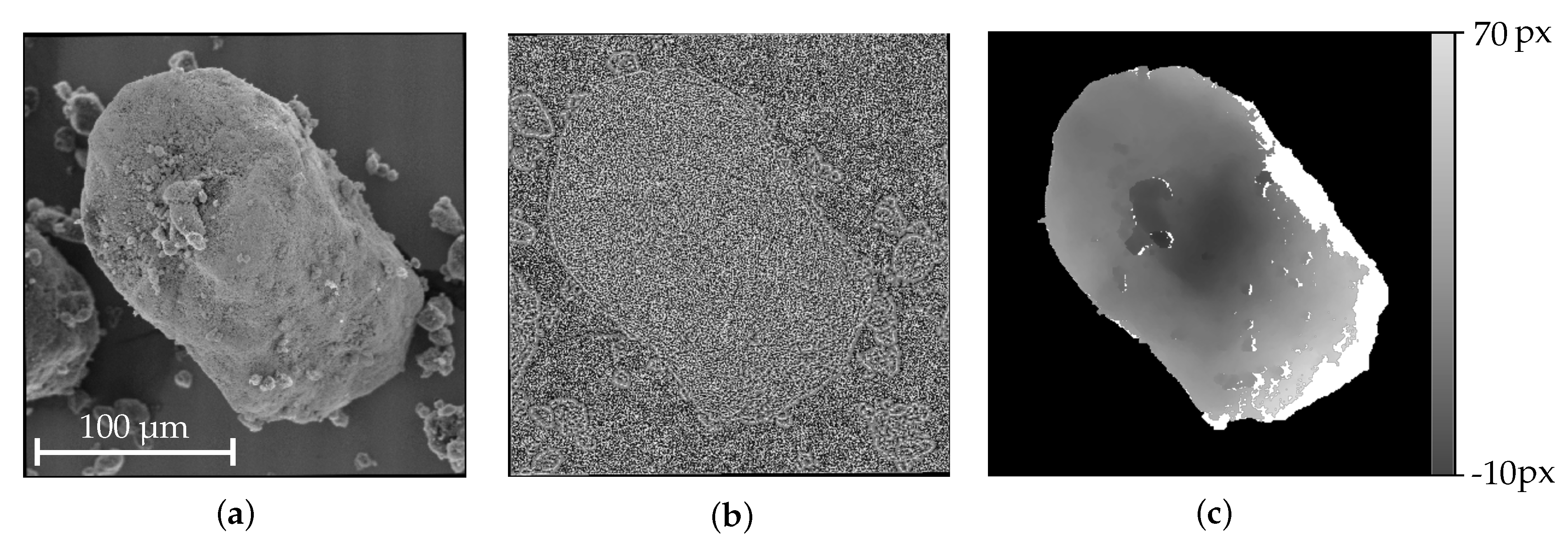
2.6. Dense Matching and Triangulation
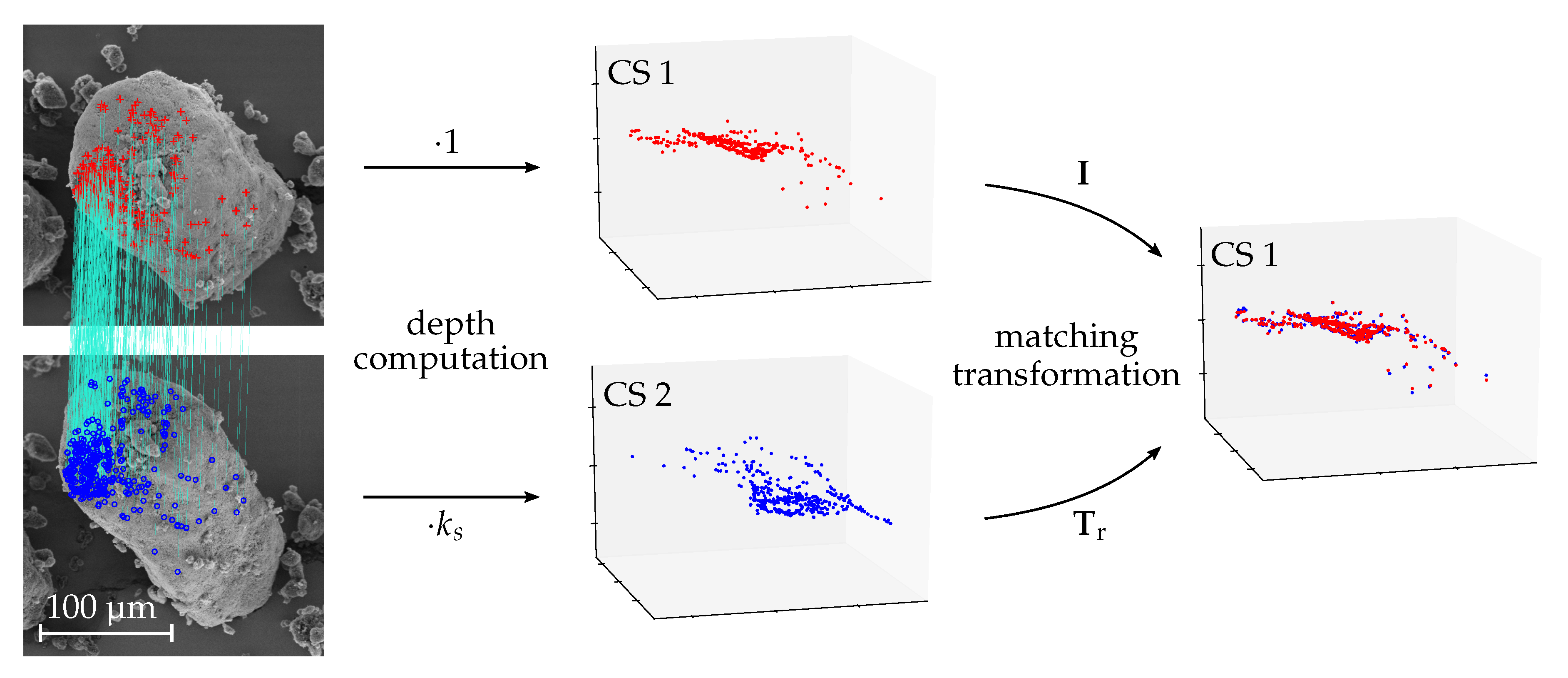
2.7. Registration
3. Results
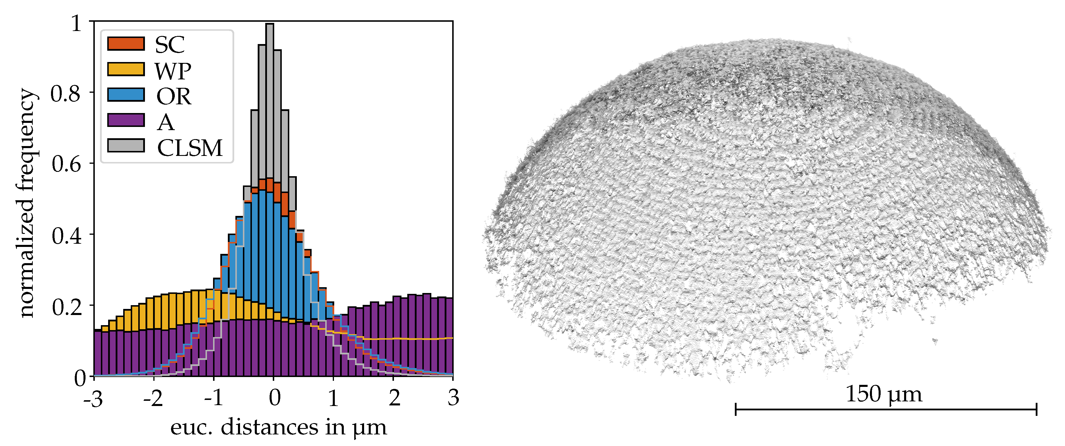
3.1. Reconstruction Evaluation
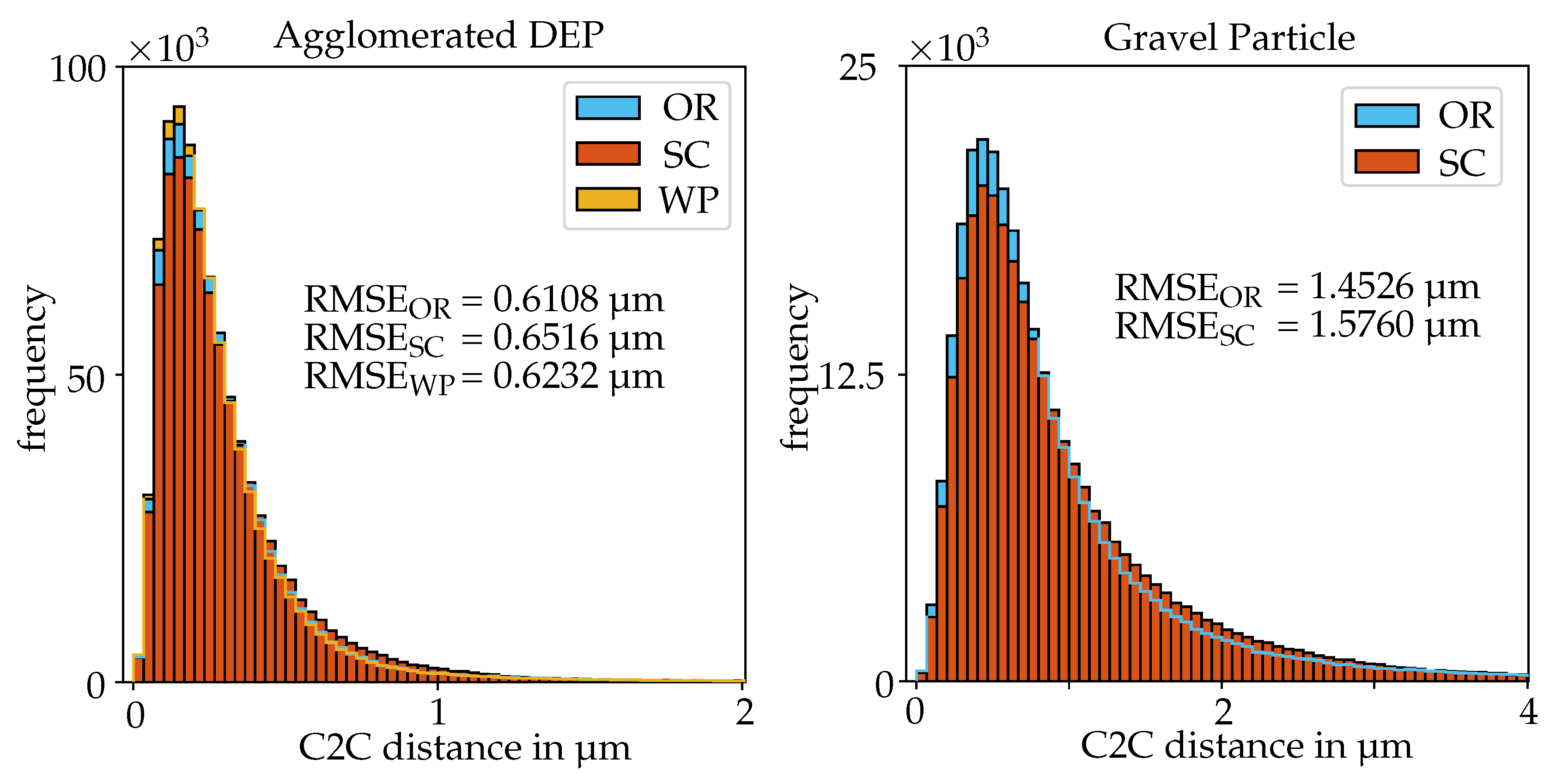
3.2. Registered Point Clouds
4. Discussion
5. Conclusions
Author Contributions
Funding
Conflicts of Interest
Abbreviations
| 2D | two-dimensional |
| 3D | three-dimensional |
| A | affine |
| C2C | cloud-to-cloud |
| CLSM | confocal laser scanning microscope |
| DEP | diesel exhaust particulate |
| DOF | depth of field |
| EVT | Everhart Thornley |
| ICP | iterative closest point |
| LSQ | least squares |
| MLESAC | maximum likelihood estimation sample consensus |
| OA | optical axis |
| OR | orthographic |
| GM | guided matching |
| RANSAC | random sample consensus |
| RMSE | root-mean-square error |
| SC | scaled orthographic |
| SEM | scanning electron microscope |
| SGBM | semi global block matching |
| SIFT | scale invariant feature transform |
| WD | working distance |
| WP | weak perspective |
References
- Liati, A.; Eggenschwiler, P.D.; Gubler, E.M.; Schreiber, D.; Aguirre, M.H. Investigation of diesel ash particulate matter: A scanning electron microscope and transmission electron microscope study. Atmos. Environ. 2012, 49, 391–402. [Google Scholar] [CrossRef]
- Fang, H.W.; Zhao, H.M.; Chen, Z.H.; Chen, M.H.; Zhang, Y.F. 3D shape and morphology characterization of sediment particles. Granul. Matter 2015, 17, 135–143. [Google Scholar] [CrossRef]
- Kirk, S.; Skepper, J.; Donald, A. Application of environmental scanning electron microscopy to determine biological surface structure. J. Microsc. 2009, 233, 205–224. [Google Scholar] [CrossRef] [PubMed]
- Griffin, B.J. A comparison of conventional Everhart-Thornley style and in-lens secondary electron detectors - a further variable in scanning electron microscopy. Scanning 2011, 33, 162–173. [Google Scholar] [CrossRef] [PubMed]
- Kratochvil, B.; Dong, L.; Zhang, L.; Nelson, B.J. Image-based 3D reconstruction using helical nanobelts for localized rotations. J. Microsc. 2010, 237, 122–135. [Google Scholar] [CrossRef] [PubMed]
- Tardif, J.-P.; Bartoli, A.; Trudeau, M.; Guilbert, N.; Roy, S. Algorithms for batch matrix factorization with application to structure-from-motion. In Proceedings of the IEEE Conference on Computer Vision and Pattern Recognition, Minneapolis, MN, USA, 17–22 June 2007; pp. 1–8. [Google Scholar]
- Xie, J. Stereomicroscopy: 3D Imaging and the Third Dimension Measurement; Application Note; Agilent Technologies: Santa Clara, CA, USA, September 2011. [Google Scholar]
- Zhu, T.; Sutton, M.A.; Li, N.; Orteu, J.-J.; Cornille, N.; Li, X.; Reynolds, A.P. Quantitative stereovision in a scanning electron microscope. Exp. Mech. 2011, 51, 97–109. [Google Scholar] [CrossRef] [Green Version]
- Tafti, A.P.; Kirkpatrick, A.B.; Alavi, Z.; Owen, H.A.; Yu, Z. Recent advances in 3D SEM surface reconstruction. Micron 2015, 78, 54–66. [Google Scholar] [CrossRef]
- Baghaie, A.; Tafti, A.P.; Owen, H.A. SD-SEM: Sparse-dense correspondence for 3D reconstruction of microscopic samples. Micron 2017, 97, 41–55. [Google Scholar] [CrossRef]
- Baghaie, A.; Tafti, A.P.; Owen, H.A.; D’Souza, R.M.; Yu, Z. Three-dimensional reconstruction of highly complex microscopic samples using scanning electron microscopy and optical flow estimation. PLoS ONE 2017, 12, e0175078. [Google Scholar] [CrossRef]
- Kudryavtsev, A.V.; Dembele, S.; Piat, N. Full 3d rotation estimation in scanning electron microscope. In Proceedings of the IEEE/RSJ International Conference on Intelligent Robots and Systems (IROS), Vancouver, BC, Canada, 24–28 September 2017; pp. 1134–1139. [Google Scholar]
- Shimshoni, I.; Basri, R.; Rivlin, E. A geometric interpretation of weak-perspective motion. IEEE Trans. Pattern Anal. Mach. Intell. 1999, 21, 252–257. [Google Scholar] [CrossRef] [Green Version]
- Kudryavtsev, A.V.; Dembélé, S.; Piat, N. Stereo-image rectification for dense 3D reconstruction in scanning electron microscope. In Proceedings of the 2017 International Conference on Manipulation, Automation and Robotics at Small Scales (MARSS), Montreal, QC, Canada, 17–21 July 2017; pp. 1–6. [Google Scholar]
- Cui, L.; Marchand, É. Scanning Electron Microscope Calibration Using a Multi-Image Non-Linear Minimization Process. Int. J. Optomechatronics 2015, 9, 151–169. [Google Scholar] [CrossRef] [Green Version]
- Ritter, M.; Hemmleb, M.; Lich, B.; Faber, P.; Hohenberg, H. SEM/FIB stage calibration with photogrammetric methods. In ISPRS Commission V Symp. 2006 (Int. Archives of Photogrammetry, Remote Sensing and Spatial Information Sciences). Available online: http://citeseerx.ist.psu.edu/viewdoc/download?doi=10.1.1.222.4938&rep=rep1&type=pdf (accessed on 25 June 2020).
- Shapiro, L.S.; Zisserman, A.; Brady, M. 3D motion recovery via affine epipolar geometry. Int. J. Comput. Vis. 1995, 16, 147–182. [Google Scholar] [CrossRef]
- Tomasi, C.; Kanade, T. Shape and motion from image streams under orthography: A factorization method. Int. J. Comput. Vis. 1992, 9, 137–154. [Google Scholar] [CrossRef]
- Poelman, C.J.; Kanade, T. A paraperspective factorization method for shape and motion recovery. IEEE Trans. Pattern Anal. Mach. Intell. 1997, 19, 206–218. [Google Scholar] [CrossRef] [Green Version]
- Quan, L. Self-calibration of an affine camera from multiple views. Int. J. Comput. Vis. 1996, 19, 93–105. [Google Scholar] [CrossRef]
- Huang, T.; Lee, C. Motion and structure from orthographic projections. IEEE Trans. Pattern Anal. Mach. Intell. 1989, 11, 536–540. [Google Scholar] [CrossRef]
- Liu, H.; Lin, H.; Yao, L. Calibration method for projector-camera-based telecentric fringe projection profilometry system. Opt. Express 2017, 25, 31492–31508. [Google Scholar] [CrossRef]
- De Franchis, C.; Meinhardt-Llopis, E.; Michel, J.; Morel, J.-M.; Facciolo, G. An automatic and modular stereo pipeline for pushbroom images. ISPRS Ann. Photogramm. Remote Sens. Spat. Inf. Sci. 2014, II-3, 49–56. [Google Scholar] [CrossRef] [Green Version]
- Thompson, D.; Mundy, J. Three-dimensional model matching from an unconstrained viewpoint. IEEE Trans. Pattern Anal. Mach. Intell. 1987, 4, 208–220. [Google Scholar]
- Lowe, D.G. Object recognition from local scale-invariant features. In Proceedings of the Seventh IEEE International Conference on Computer Vision, Kerkyra, Greece, 20–27 September 1999; pp. 1150–1157. [Google Scholar]
- Tafti, A.P.; Baghaie, A.; Kirkpatrick, A.B.; Holz, J.D.; Owen, H.A.; D’Souza, R.M.; Yu, Z. A comparative study on the application of SIFT, SURF, BRIEF and ORB for 3D surface reconstruction of electron microscopy images. Comput. Methods Biomech. Biomed. Eng. Imaging Vis. 2018, 6, 17–30. [Google Scholar] [CrossRef]
- Arandjelović, R.; Zisserman, A. Three things everyone should know to improve object retrieval. In Proceedings of the IEEE Conference on Computer Vision and Pattern Recognition, Providence, RI, USA, 16–21 June 2012; pp. 2911–2918. [Google Scholar]
- Hartley, R.; Zisserman, A. Multiple View Geometry in Computer Vision; Cambridge University Press: Cambridge, UK, 2003; pp. 349–351. [Google Scholar]
- Joy, D.C. Noise and its effects on the low-voltage SEM. In Biological Low-Voltage Scanning Electron Microscopy; Springer Science and Business Media LLC: Berlin/Heidelberg, Germany, 2007; pp. 129–144. [Google Scholar]
- Torr, P.; Zisserman, A. MLESAC: A new robust estimator with application to estimating image geometry. Comput. Vis. Image Underst. 2000, 78, 138–156. [Google Scholar] [CrossRef] [Green Version]
- Tordoff, B.J.; Murray, D.W. Guided-MLESAC: Faster image transform estimation by using matching priors. IEEE Trans. Pattern Anal. Mach. Intell. 2005, 27, 1523–1535. [Google Scholar] [CrossRef] [PubMed] [Green Version]
- Fischler, M.A.; Bolles, R.C. Random sample consensus: A paradigm for model fitting with applications to image analysis and automated cartography. Commun. ACM 1981, 24, 381–395. [Google Scholar] [CrossRef]
- Toshihiko, M.; Kanade, T. A sequential factorization method for recovering shape and motion from image streams. IEEE Trans. Pattern Anal. Mach. Intell. 1997, 19, 858–867. [Google Scholar]
- Higham, N.J. Computing a nearest symmetric positive semidefinite matrix. Linear Algebra Its Appl. 1988, 103, 103–118. [Google Scholar] [CrossRef]
- Hartley, R. Theory and practice of projective rectification. Int. J. Comput. Vis. 1999, 35, 115–127. [Google Scholar] [CrossRef]
- Hirschmuller, H. Stereo processing by semiglobal matching and mutual information. IEEE Trans. Pattern Anal. Mach. Intell. 2007, 30, 328–341. [Google Scholar] [CrossRef]
- Zabih, R.; Woodfill, J. Non-parametric local transforms for computing visual correspondence. Eur. Conf. Comput. Vis. 1994, 801, 151–158. [Google Scholar]
- Birchfield, S.; Tomasi, C. A pixel dissimilarity measure that is insensitive to image sampling. IEEE Trans. Pattern Anal. Mach. Intell. 1998, 20, 401–406. [Google Scholar] [CrossRef] [Green Version]
- Rother, C.; Kolmogorov, V.; Blake, A. “GrabCut” interactive foreground extraction using iterated graph cuts. Acm Trans. Graph. 2004, 23, 309–314. [Google Scholar] [CrossRef]
- Yu, G.; Morel, J.M. A fully affine invariant image comparison method. In Proceedings of the IEEE International Conference on Acoustics, Speech and Signal Processing, Taipei, Taiwan, 19–24 April 2009; pp. 1597–1600. [Google Scholar]
- Arun, K.S.; Huang, T.S.; Blostein, S.D. Least-squares fitting of two 3-D point sets. IEEE Trans. Pattern Anal. Mach. Intell. 1987, 698–700. [Google Scholar] [CrossRef] [PubMed] [Green Version]
- Chetverikov, D.; Svirko, D.; Stepanov, D.; Krsek, P. The trimmed iterative closest point algorithm. In Proceedings of the Object Recognition Supported by User Interaction for Service Robots, Quebec City, QC, Canada, 11–15 August 2002; pp. 545–548. [Google Scholar]
- Reimer, L. Scanning Electron Microscopy: Physics of Image Formation and Microanalysis; Springer: Heidelberg, Germany, 1998; p. 11. [Google Scholar]
- Kazhdan, M.; Bolitho, M.; Hoppe, H. Poisson surface reconstruction. In Proceedings of the Fourth Eurographics Symposium on Geometry Processing, Cagliari, Sardinia, Italy, 26–28 June 2006. [Google Scholar]
- Töberg, S.; Reithmeier, E. Dense structure and motion recovery from scanning electron microscope image sequences based on factorization. In Proceedings of the Twelfth International Conference on Machine Vision (ICMV 2019), Amsterdam, The Netherlands, 16–18 November 2019. [Google Scholar]
- Blonquist, K.F.; Pack, R.T. A bundle adjustment approach with inner constraints for the scaled orthographic projection. Isprs J. Photogramm. Remote. Sens. 2011, 66, 919–926. [Google Scholar] [CrossRef]


| Method | Sphere 1 mm | Sphere 300 µm | Sphere 300 µm | Pebble Stone | DEP I | DEP II |
|---|---|---|---|---|---|---|
| m | 76 | 544 | 296 | 630 | 963 | 463 |
| mag | 60 | 200 | 200 | 150 | 400 | 1000 |
| 10 | ||||||
| None | 2.1220 | 973.54 | 907.54 | 1.7494 | 7.9539 | 46303 |
| Rigid | 0.9592 | 0.7864 | 1.1596 | 0.4086 | 0.3235 | 2.2329 |
| Similarity | 0.5992 | 0.6260 | 0.6179 | 0.3639 | 0.3167 | 0.7635 |
| Method | in µm | RMSE in µm | c | s | ||||
|---|---|---|---|---|---|---|---|---|
| Orthographic (OR) | 146.70 | 0.8748 | 1 | 1 | 1 | 1 | 1 | 0 |
| Scaled Orthographic (SC) | 151.93 | 0.8247 | 1 | 0.9992 | 0.9984 | 0.9999 | 1 | 0 |
| Weak Perspective (WP) | 149.49 | 3.6932 | 1 | 0.9993 | 0.9984 | 0.9984 | 1.1632 | 0 |
| Affine (A) | 203.16 | 20.1177 | 1 | 0.9994 | 0.9984 | 0.9999 | 0.5879 | −0.1032 |
| Weak Perspective | 155.54 | 0.8531 | 1 | 0.9993 | 0.9984 | 0.9984 | 1 | 0 |
| Affine | 151.97 | 2.8265 | 1 | 0.9994 | 0.9984 | 0.9999 | 1 | 0 |
| CLSM | 150.86 | 0.5251 | - | - | - | - | - | - |
| Method | ||||||||||||
|---|---|---|---|---|---|---|---|---|---|---|---|---|
| Orthographic | 0.12 | 4.67 | 0.03 | −0.50 | 9.36 | −0.03 | −0.51 | 14.03 | −0.02 | |||
| Scaled Orthographic | 0.13 | 5.03 | 0.03 | −0.54 | 10.08 | −0.04 | −0.55 | 15.11 | −0.03 | |||
| Weak Perspective | 0.16 | 5.26 | 0.03 | −0.65 | 10.51 | 0.02 | −0.66 | 15.68 | 0.01 | |||
| Affine | −0.44 | 4.99 | 0.01 | −1.36 | 9.99 | 0.11 | −1.91 | 14.99 | 0.22 |
| Image Sequence | Mag. | m | |||||||
|---|---|---|---|---|---|---|---|---|---|
| Chalked Sphere I | 60 | 207 | 1.0025 | 1.0024 | 1.0012 | 0.0064 | 1.1498 | 0.6543 | 0.0193 |
| Chalked Sphere II | 60 | 50 | 1.0024 | 1.0023 | 1.0097 | 0.0157 | 0.7606 | 0.3027 | 0.0464 |
| Gravel Particle | 150 | 395 | 0.9996 | 0.9987 | 0.9977 | 0.0042 | 0.7067 | 0.0049 | −0.0225 |
| Sphere 300 µm | 200 | 72 | 0.9992 | 0.9984 | 0.9999 | 0.0025 | 1.1632 | 0.5879 | −0.1032 |
| DEP Agglomerate | 400 | 400 | 0.9989 | 1.0004 | 0.9987 | 0.0027 | 0.9975 | 0.1658 | −0.0119 |
| Image Sequence | Method | ||||||||
|---|---|---|---|---|---|---|---|---|---|
| Sphere 300 µm | OR | 0.33 | 0.64 | 0.97 | 1.97 | ||||
| SC | 0.03 | 0.08 | 0.11 | 0.22 | |||||
| Chalked Sphere I | OR | 0.42 | 0.93 | 1.71 | 3.06 | ||||
| SC | 0.12 | 0.17 | 0.01 | 0.30 | |||||
| Chalked Sphere II | OR | 0.81 | 1.55 | 1.94 | 4.03 | ||||
| SC | 0.02 | 0.11 | 0.56 | 0.69 |
© 2020 by the authors. Licensee MDPI, Basel, Switzerland. This article is an open access article distributed under the terms and conditions of the Creative Commons Attribution (CC BY) license (http://creativecommons.org/licenses/by/4.0/).
Share and Cite
Töberg, S.; Reithmeier, E. Quantitative 3D Reconstruction from Scanning Electron Microscope Images Based on Affine Camera Models. Sensors 2020, 20, 3598. https://doi.org/10.3390/s20123598
Töberg S, Reithmeier E. Quantitative 3D Reconstruction from Scanning Electron Microscope Images Based on Affine Camera Models. Sensors. 2020; 20(12):3598. https://doi.org/10.3390/s20123598
Chicago/Turabian StyleTöberg, Stefan, and Eduard Reithmeier. 2020. "Quantitative 3D Reconstruction from Scanning Electron Microscope Images Based on Affine Camera Models" Sensors 20, no. 12: 3598. https://doi.org/10.3390/s20123598