Triplet Loss Guided Adversarial Domain Adaptation for Bearing Fault Diagnosis


Abstract
:1. Introduction
- We propose a novel and effective unsupervised domain adaptation approach for bearing fault diagnosis. Data-level and class-level alignment between the source domain and target domain are both considered.
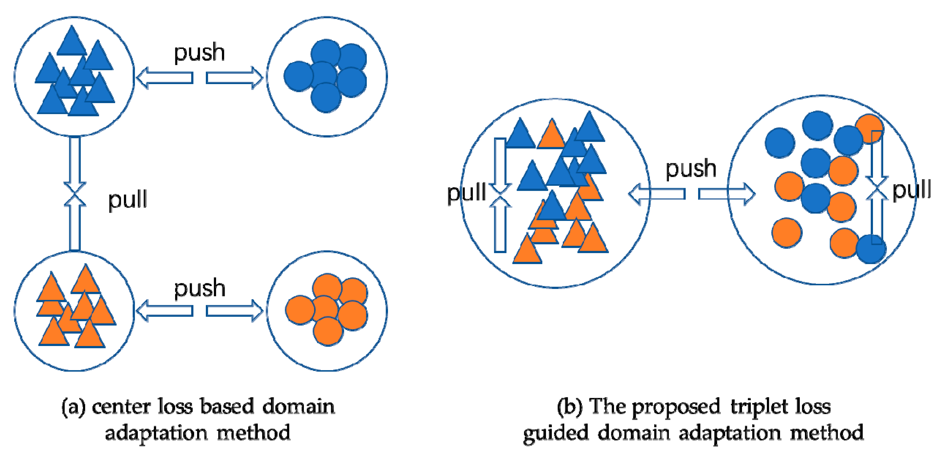
- We propose to use triplet loss to achieve better intra-class compactness and inter-class separability for samples from both domains simultaneously.
- Extensive experiments are performed to validate the efficacy of the proposed method. In addition to transfer learning between different working conditions on CWRU dataset and Paderborn dataset, we also validate the transfer learning tasks between different sensor locations on CWRU dataset.
2. Backgrounds
2.1. Unsupervised Domain Adaptation
2.2. Wasserstein Distance
2.3. Deep Metric Learning
3. Proposed Method
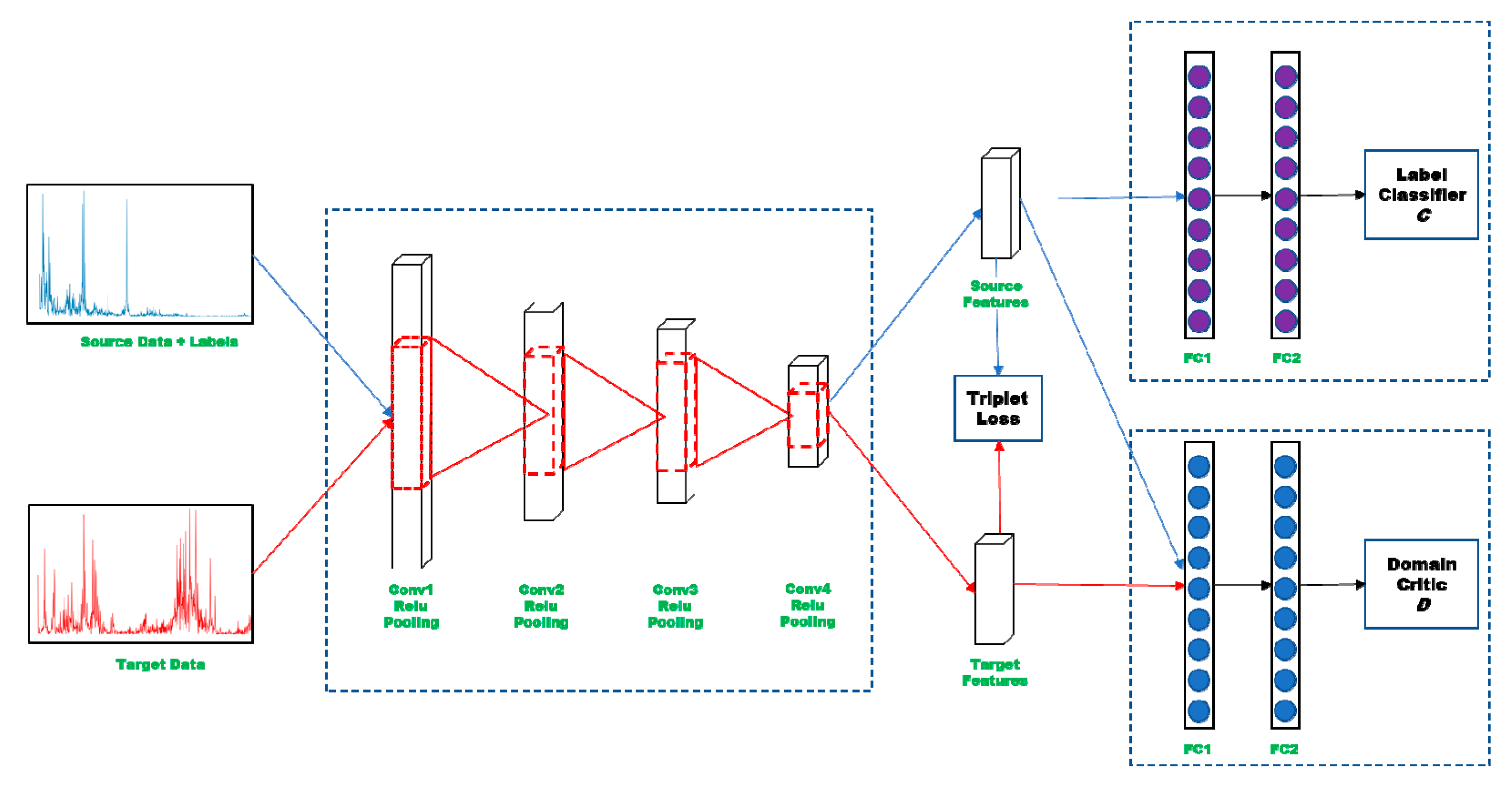
3.1. Overview
3.2. Domain-Level Alignment by Wasserstein Distance
3.3. Class-level Alignment with Triplet Loss
4. Experiments
4.1. Implementation Details
- Wasserstein distance guided representation learning (WDGRL) proposed by Shen et al. [34]. Wasserstein distance of representations learned from feature extractor is minimized to learn domain-invariant representations through adversarial learning.
- Deep convolutional transfer learning network (DCTLN) proposed by Lei et al. [31]. Both adversarial learning and MMD loss are employed to minimize the domain discrepancy.
- Transfer component analysis (TCA) proposed by Pan et al. [26].
- CNN: The neural network trained on labeled data from the source domain is used to classify the target domain directly without domain adaptation.
- DeepCoral proposed by Sun et al. [6]. Mean and covariance of feature representations are matched to minimize domain shift.
- Deep domain confusion (DDC) proposed by Tzeng et al. [25]. DDC uses one adaptation layer and domain confusion loss to learn domain invariant representations.
- Deep adaptation network (DAN) proposed by Long et al. [27]. Feature distributions are aligned through minimizing multi-kernel MMD distance between domains.
4.2. Case 1: Results and Analysis of CWRU Dataset
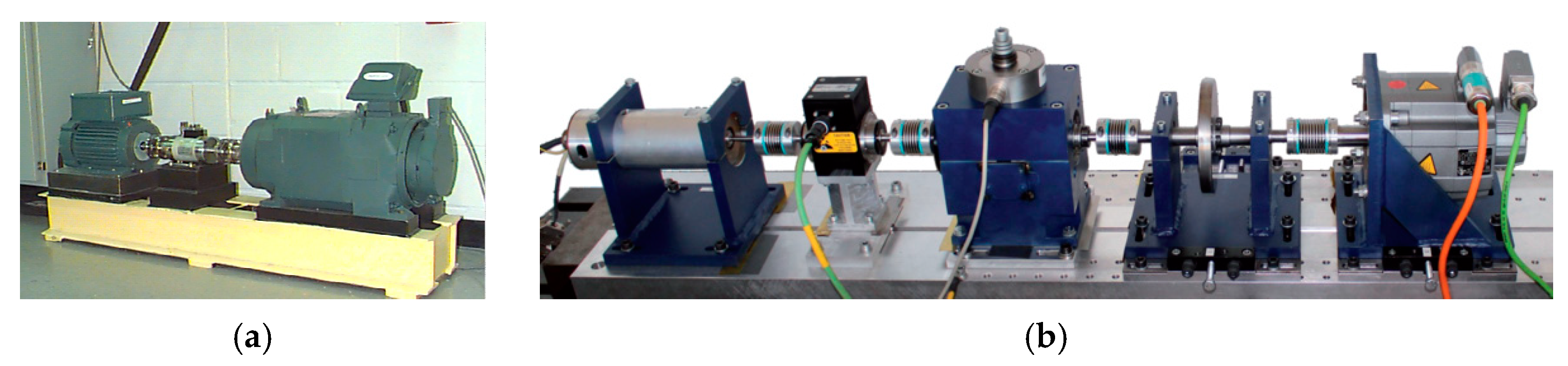
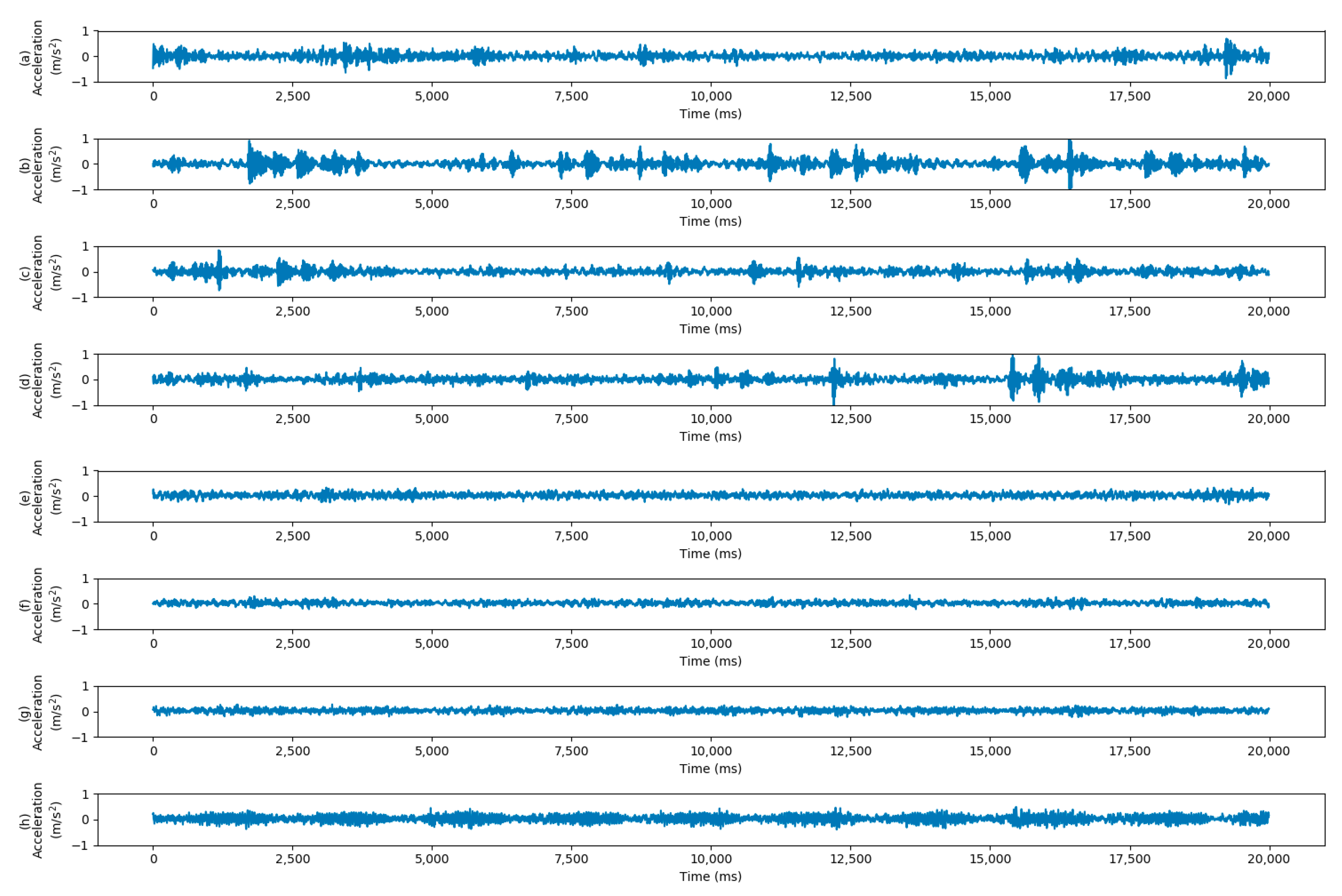
4.2.1. Dataset and Implementation
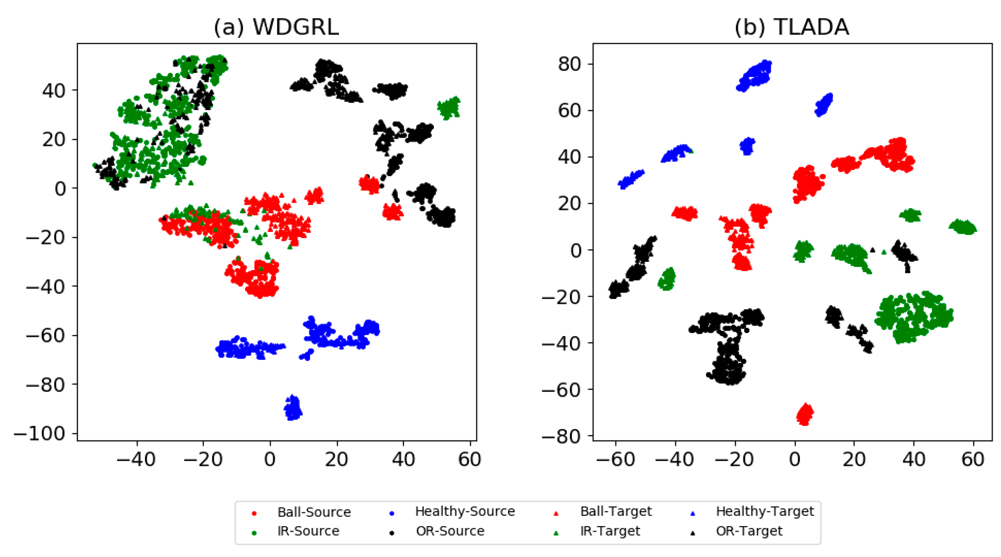
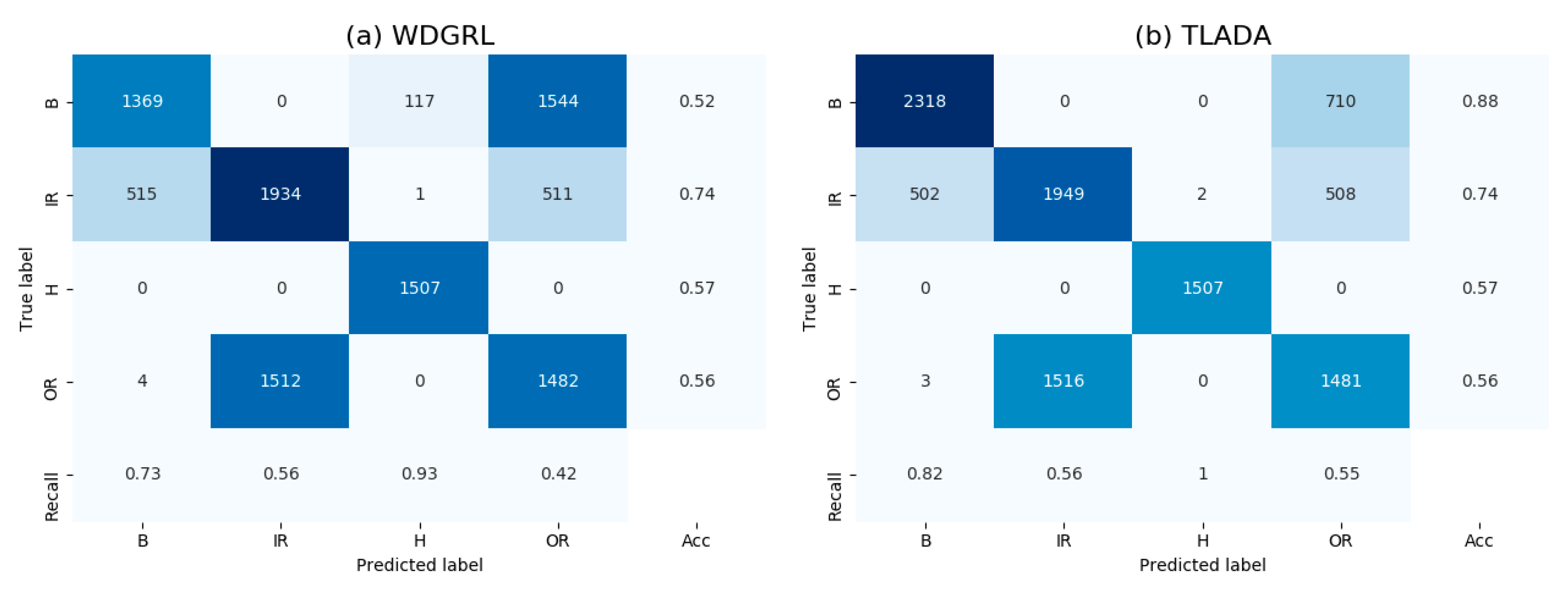
4.2.2. Results and Analysis
4.3. Case 2: Results and Analysis of Paderborn Dataset
4.3.1. Dataset and Experiment
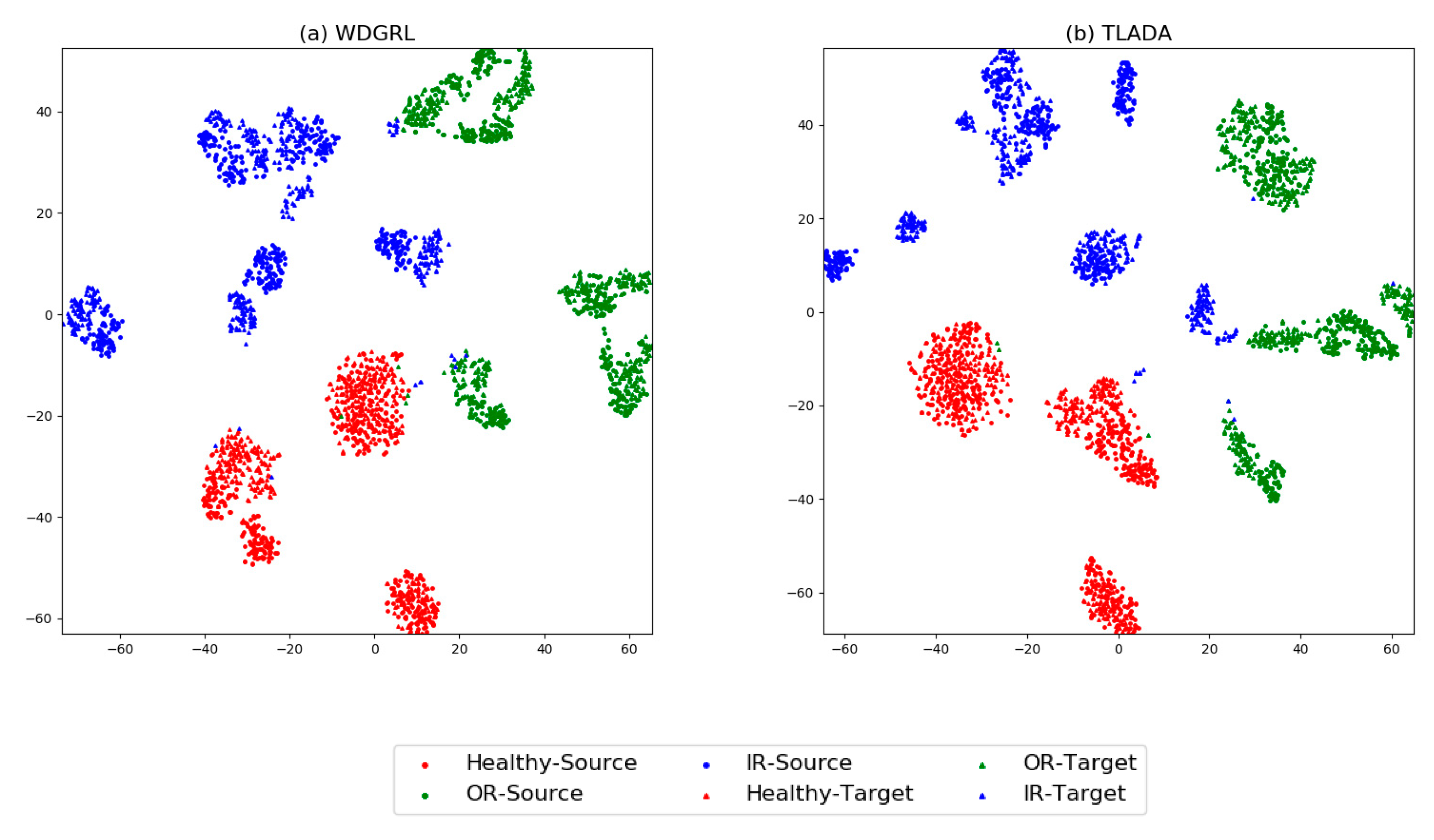
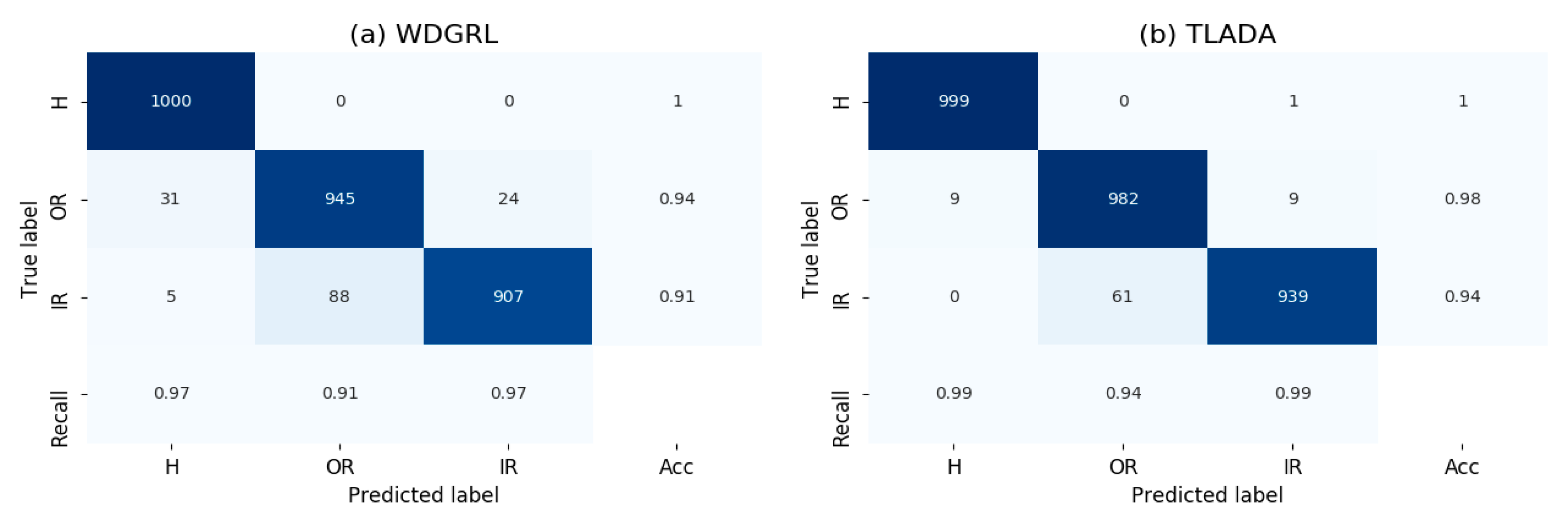
4.3.2. Results
4.4. Analysis
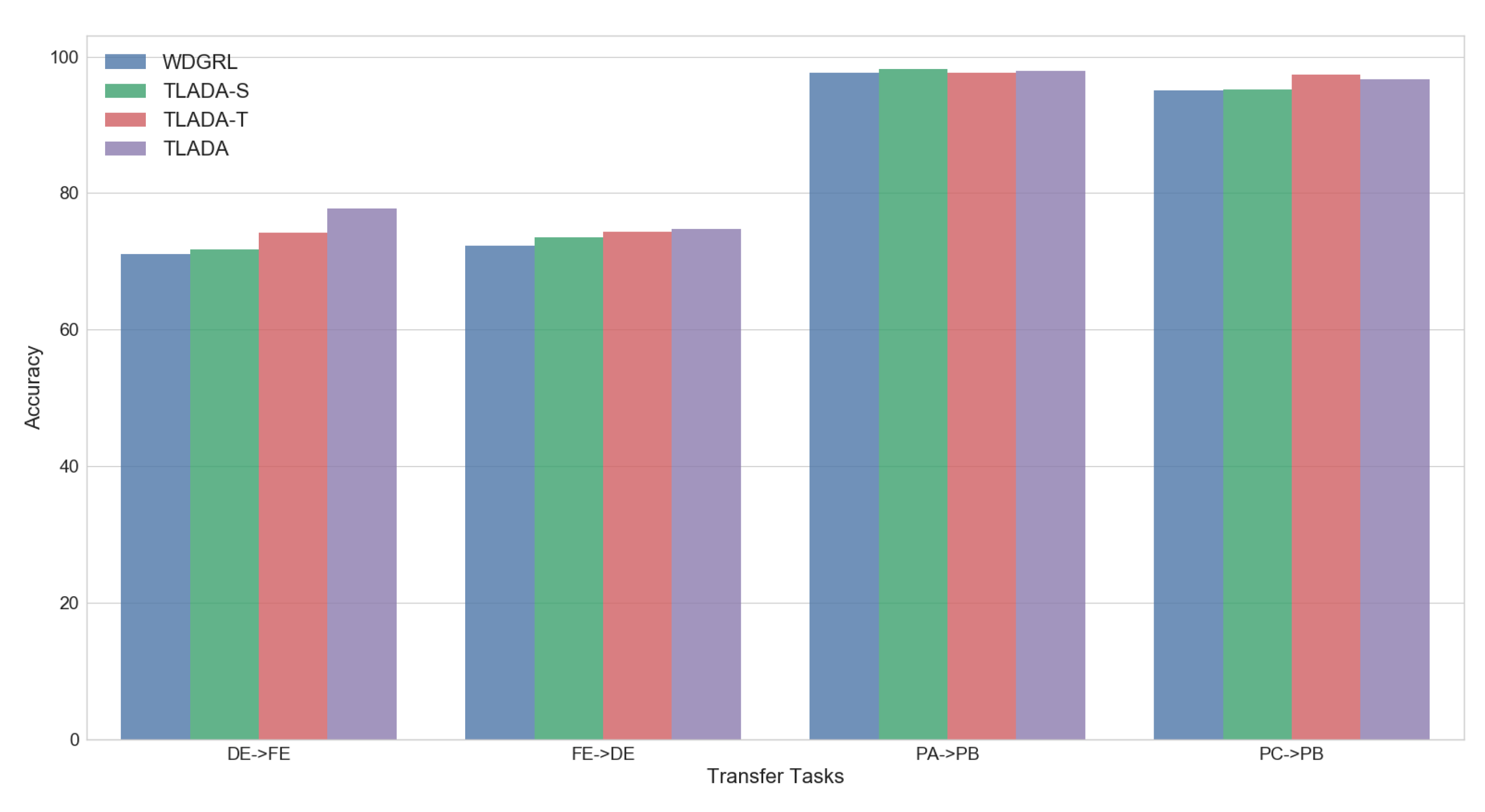
4.4.1. Ablation Analysis
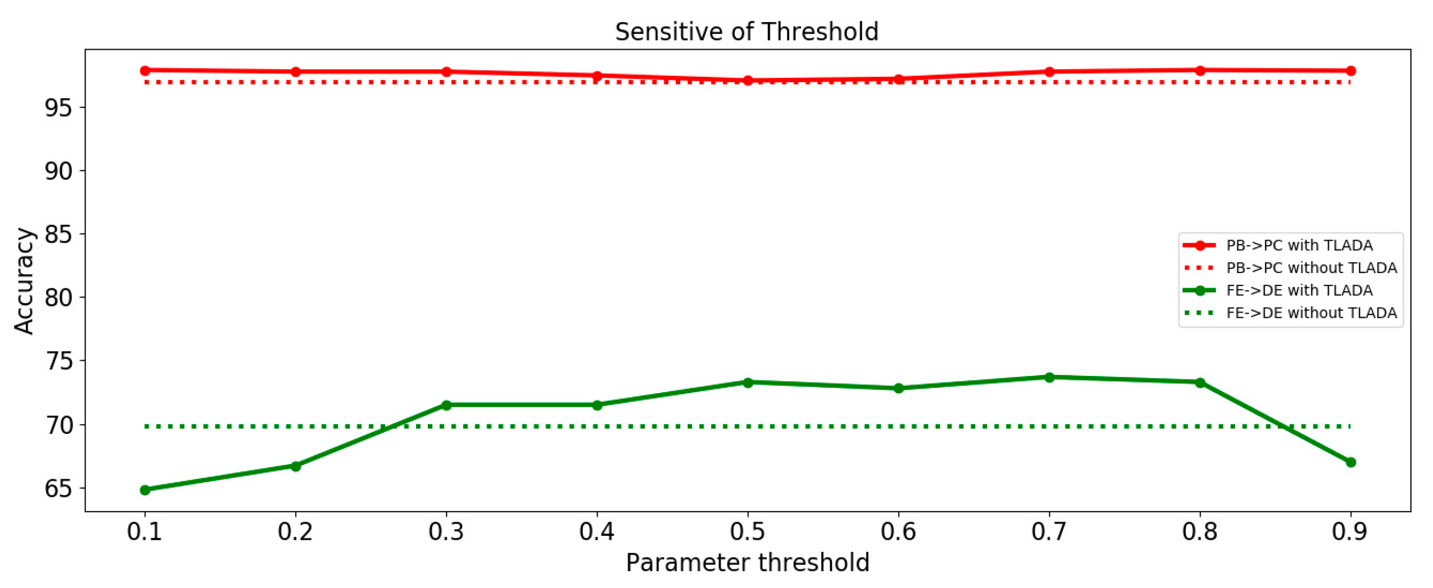
4.4.2. Parameter Sensitive Analysis
4.4.3. Computational Cost
5. Conclusions
Author Contributions
Funding
Conflicts of Interest
References
- Liu, R.; Yang, B.; Zio, E.; Chen, X. Artificial intelligence for fault diagnosis of rotating machinery: A review. Mech. Syst. Signal Process. 2018, 108, 33–47. [Google Scholar] [CrossRef]
- Khan, S.; Yairi, T. A review on the application of deep learning in system health management. Mech. Syst. Signal Process. 2018, 107, 241–265. [Google Scholar] [CrossRef]
- Ben-David, S.; Blitzer, J.; Crammer, K.; Kulesza, A.; Pereira, F.; Vaughan, J.W. A theory of learning from different domains. Mach. Learn. 2010, 79, 151–175. [Google Scholar] [CrossRef] [Green Version]
- Pan, S.J.; Yang, Q. A survey on transfer learning. IEEE Trans. Knowl. Data Eng. 2009, 22, 1345–1359. [Google Scholar] [CrossRef]
- Zhang, B.; Li, W.; Li, X.-L.; Ng, S.-K. Intelligent fault diagnosis under varying working conditions based on domain adaptive convolutional neural networks. IEEE Access 2018, 6, 66367–66384. [Google Scholar] [CrossRef]
- Sun, B.; Saenko, K. Deep coral: Correlation alignment for deep domain adaptation. In Proceedings of the European Conference on Computer Vision, Amsterdam, The Netherlands, 11–14 October 2016; pp. 443–450. [Google Scholar]
- Gretton, A.; Borgwardt, K.M.; Rasch, M.J.; Schölkopf, B.; Smola, A. A kernel two-sample test. J. Mach. Learn. Res. 2012, 13, 723–773. [Google Scholar]
- Lu, W.; Liang, B.; Cheng, Y.; Meng, D.; Yang, J.; Zhang, T. Deep model based domain adaptation for fault diagnosis. IEEE Trans. Ind. Electron. 2016, 64, 2296–2305. [Google Scholar] [CrossRef]
- Wen, L.; Gao, L.; Li, X. A new deep transfer learning based on sparse auto-encoder for fault diagnosis. IEEE Trans. Syst. Man Cybern. Syst. 2017, 49, 136–144. [Google Scholar] [CrossRef]
- Li, X.; Zhang, W.; Ding, Q.; Sun, J.-Q. Multi-Layer domain adaptation method for rolling bearing fault diagnosis. Signal Process. 2019, 157, 180–197. [Google Scholar] [CrossRef] [Green Version]
- Wang, Q.; Michau, G.; Fink, O. Domain Adaptive Transfer Learning for Fault Diagnosis. arXiv 2019, arXiv:1905.06004. [Google Scholar]
- Ganin, Y.; Ustinova, E.; Ajakan, H.; Germain, P.; Larochelle, H.; Laviolette, F.; Marchand, M.; Lempitsky, V. Domain-adversarial training of neural networks. J. Mach. Learn. Res. 2016, 17, 2030–2096. [Google Scholar]
- Tzeng, E.; Hoffman, J.; Saenko, K.; Darrell, T. Adversarial discriminative domain adaptation. In Proceedings of the IEEE Conference on Computer Vision and Pattern Recognition, Honolulu, HI, USA, 21–26 July 2017; pp. 7167–7176. [Google Scholar]
- Goodfellow, I.; Pouget-Abadie, J.; Mirza, M.; Xu, B.; Warde-Farley, D.; Ozair, S.; Courville, A.; Bengio, Y. Generative adversarial nets. In Proceedings of the Advances in Neural Information Processing Systems, Montreal, QC, Canada, 8–13 December 2014; pp. 2672–2680. [Google Scholar]
- Cheng, C.; Zhou, B.; Ma, G.; Wu, D.; Yuan, Y. Wasserstein Distance based Deep Adversarial Transfer Learning for Intelligent Fault Diagnosis. arXiv 2019, arXiv:1903.06753. [Google Scholar]
- Zhang, M.; Wang, D.; Lu, W.; Yang, J.; Li, Z.; Liang, B. A Deep Transfer Model With Wasserstein Distance Guided Multi-Adversarial Networks for Bearing Fault Diagnosis Under Different Working Conditions. IEEE Access 2019, 7, 65303–65318. [Google Scholar] [CrossRef]
- Motiian, S.; Jones, Q.; Iranmanesh, S.; Doretto, G. Few-shot adversarial domain adaptation. In Proceedings of the Advances in Neural Information Processing Systems, Long Beach, CA, USA, 4–9 December 2017; pp. 6670–6680. [Google Scholar]
- Zhang, Y.; Zhang, Y.; Wang, Y.; Tian, Q. Domain-Invariant Adversarial Learning for Unsupervised Domain Adaption. arXiv 2018, arXiv:1811.12751. [Google Scholar]
- Chen, D.-D.; Wang, Y.; Yi, J.; Chen, Z.; Zhou, Z.-H. Joint Semantic Domain Alignment and Target Classifier Learning for Unsupervised Domain Adaptation. arXiv 2019, arXiv:1906.04053. [Google Scholar]
- Chen, C.; Chen, Z.; Jiang, B.; Jin, X. Joint domain alignment and discriminative feature learning for unsupervised deep domain adaptation. In Proceedings of the AAAI Conference on Artificial Intelligence, Honolulu, HI, USA, 27 January–1 February 2019; pp. 3296–3303. [Google Scholar]
- Li, X.; Zhang, W.; Ding, Q. A robust intelligent fault diagnosis method for rolling element bearings based on deep distance metric learning. Neurocomputing 2018, 310, 77–95. [Google Scholar] [CrossRef]
- Xie, S.; Zheng, Z.; Chen, L.; Chen, C. Learning semantic representations for unsupervised domain adaptation. In Proceedings of the International Conference on Machine Learning, Jinan, China, 26–28 May 2018; pp. 5419–5428. [Google Scholar]
- Deng, W.; Zheng, L.; Jiao, J. Domain Alignment with Triplets. arXiv 2018, arXiv:1812.00893. [Google Scholar]
- Long, M.; Zhu, H.; Wang, J.; Jordan, M.I. Deep transfer learning with joint adaptation networks. In Proceedings of the 34th International Conference on Machine Learning, Sydney, Australia, 6–11 August 2017; Volume 70, pp. 2208–2217. [Google Scholar]
- Tzeng, E.; Hoffman, J.; Zhang, N.; Saenko, K.; Darrell, T. Deep domain confusion: Maximizing for domain invariance. arXiv 2014, arXiv:1412.3474. [Google Scholar]
- Pan, S.J.; Tsang, I.W.; Kwok, J.T.; Yang, Q. Domain adaptation via transfer component analysis. IEEE Trans. Neural Netw. 2010, 22, 199–210. [Google Scholar] [CrossRef] [Green Version]
- Long, M.; Cao, Y.; Wang, J.; Jordan, M.I. Learning transferable features with deep adaptation networks. arXiv 2015, arXiv:1502.02791. [Google Scholar]
- Yang, B.; Lei, Y.; Jia, F.; Xing, S. An intelligent fault diagnosis approach based on transfer learning from laboratory bearings to locomotive bearings. Mech. Syst. Signal Process. 2019, 122, 692–706. [Google Scholar] [CrossRef]
- Han, T.; Liu, C.; Yang, W.; Jiang, D. A novel adversarial learning framework in deep convolutional neural network for intelligent diagnosis of mechanical faults. Knowl. Based Syst. 2019, 165, 474–487. [Google Scholar] [CrossRef]
- Zhang, B.; Li, W.; Hao, J.; Li, X.-L.; Zhang, M. Adversarial adaptive 1-D convolutional neural networks for bearing fault diagnosis under varying working condition. arXiv 2018, arXiv:1805.00778. [Google Scholar]
- Guo, L.; Lei, Y.; Xing, S.; Yan, T.; Li, N. Deep convolutional transfer learning network: A new method for intelligent fault diagnosis of machines with unlabeled data. IEEE Trans. Ind. Electron. 2018, 66, 7316–7325. [Google Scholar] [CrossRef]
- Arjovsky, M.; Chintala, S.; Bottou, L. Wasserstein gan. arXiv 2017, arXiv:1701.07875. [Google Scholar]
- Gulrajani, I.; Ahmed, F.; Arjovsky, M.; Dumoulin, V.; Courville, A.C. Improved training of wasserstein gans. In Proceedings of the Advances in Neural Information Processing Systems, Long Beach, CA, USA, 4–9 December 2017; pp. 5767–5777. [Google Scholar]
- Shen, J.; Qu, Y.; Zhang, W.; Yu, Y. Wasserstein distance guided representation learning for domain adaptation. arXiv 2017, arXiv:1707.01217. [Google Scholar]
- Wen, Y.; Zhang, K.; Li, Z.; Qiao, Y. A discriminative feature learning approach for deep face recognition. In Proceedings of the European Conference on Computer Vision, Amsterdam, The Netherlands, 11–14 October 2016; pp. 499–515. [Google Scholar]
- Sun, Y.; Chen, Y.; Wang, X.; Tang, X. Deep learning face representation by joint identification-verification. In Proceedings of the Advances in Neural Information Processing Systems, Montreal, QC, Canada, 8–13 December 2014; pp. 1988–1996. [Google Scholar]
- Schroff, F.; Kalenichenko, D.; Philbin, J. Facenet: A unified embedding for face recognition and clustering. In Proceedings of the IEEE Conference on Computer Vision and Pattern Recognition, Boston, MA, USA, 7–12 June 2015; pp. 815–823. [Google Scholar]
- Hoffer, E.; Ailon, N. Deep metric learning using triplet network. In Proceedings of the International Workshop on Similarity-Based Pattern Recognition, Copenhagen, Denmark, 12–14 October 2015; pp. 84–92. [Google Scholar]
- Zhang, W.; Peng, G.; Li, C.; Chen, Y.; Zhang, Z. A new deep learning model for fault diagnosis with good anti-noise and domain adaptation ability on raw vibration signals. Sensors 2017, 17, 425. [Google Scholar] [CrossRef]
- Paderborn University Bearing Data Center. Available online: https://mb.uni-Paderborn.de/kat/forschung/datacenter/bearing-datacenter (accessed on 10 October 2019).
- Lessmeier, C.; Kimotho, J.K.; Zimmer, D.; Sextro, W. Condition monitoring of bearing damage in electromechanical drive systems by using motor current signals of electric motors: A benchmark data set for data-driven classification. In Proceedings of the European Conference of the Prognostics and Health Management Society, Bilbao, Spain, 5–8 July 2016; pp. 5–8. [Google Scholar]


| Algorithm: TLADA |
|---|
| Require: source data ; target data ; minibatch size m; critic training step n; learning rate for domain critic a1; learning rate for classification and feature learning a2; |
|
| Component | Layer Type | Kernel | Stride | Channel | Activation |
|---|---|---|---|---|---|
| Feature Extractor | Convolution 1 | 32 × 1 | 2 × 1 | 8 | Relu |
| Pooling 1 | 2 × 1 | 2 × 1 | 8 | ||
| Convolution 2 | 16 × 1 | 2 × 1 | 16 | Relu | |
| Pooling 2 | 2 × 1 | 2 × 1 | 16 | ||
| Convolution 3 | 8 × 1 | 2 × 1 | 32 | Relu | |
| Pooling 3 | 2 × 1 | 2 × 1 | 32 | ||
| Convolution 4 | 3 × 1 | 2 × 1 | 32 | Relu | |
| Pooling 4 | 2 × 1 | 2 × 1 | 32 | ||
| Classifier | Fully-connected 1 | 500 | 1 | Relu | |
| Fully-connected 2 | C1 | 1 | Relu | ||
| Critic | Fully-connected 1 | 500 | 1 | Relu | |
| Fully-connected 2 | 1 | 1 | Relu |
| Datasets | Working Conditions | # of Categories | Samples in Each Category | Category Details |
|---|---|---|---|---|
| DE0 | 0 | 10 | 1000 | Health, Inner 0.007, Inner 0.014, Inner 0.021, Outer 0.007, Outer 0.014, Outer 0.021, Ball 0.007, Ball 0.014, Ball 0.021 |
| DE1 | 1 | 10 | 1000 | |
| DE2 | 2 | 10 | 1000 | |
| DE3 | 3 | 10 | 1000 | |
| DE | 1/2/3 | 4 | 6000 | Health, Inner (0.007, 0.021), Outer (0.007, 0.021), Ball (0.007, 0.021) |
| FE | 1/2/3 | 4 | 6000 |
| Task | TCA | CNN | Deep CORAL | DDC | DAN | DCTLN | WDGRL | TLADA |
|---|---|---|---|---|---|---|---|---|
| DE0 -> DE1 | 62.50 | 95.07 | 98.11 | 98.24 | 99.38 | 99.99 | 99.71 | 99.68 |
| DE0 -> DE2 | 65.54 | 79.28 | 83.35 | 80.25 | 90.04 | 99.99 | 98.96 | 99.81 |
| DE0 -> DE3 | 74.49 | 63.49 | 75.58 | 74.17 | 91.48 | 93.38 | 99.22 | 99.61 |
| DE1 -> DE0 | 63.63 | 79.99 | 90.04 | 88.96 | 99.88 | 99.99 | 99.67 | 99.82 |
| DE1 -> DE2 | 64.37 | 89.33 | 99.25 | 91.17 | 99.99 | 100 | 99.88 | 100 |
| DE1 -> DE3 | 79.88 | 58.48 | 87.81 | 83.70 | 99.47 | 100 | 99.16 | 99.51 |
| DE2 -> DE0 | 59.05 | 90.96 | 86.18 | 67.90 | 94.11 | 95.05 | 95.25 | 98.32 |
| DE2 -> DE1 | 63.39 | 88.81 | 89.31 | 90.64 | 95.26 | 99.99 | 93.16 | 96.61 |
| DE2 -> DE3 | 65.57 | 87.15 | 98.07 | 88.28 | 100 | 100 | 99.99 | 100 |
| DE3 -> DE0 | 72.92 | 68.09 | 76.49 | 74.60 | 91.21 | 89.26 | 90.75 | 94.37 |
| DE3 -> DE1 | 68.93 | 75.11 | 79.61 | 74.77 | 89.95 | 86.17 | 95.75 | 95.97 |
| DE3 -> DE2 | 63.97 | 89.84 | 90.66 | 96.70 | 100 | 99.98 | 99.46 | 100 |
| average | 67.02 | 80.47 | 87.87 | 84.12 | 95.90 | 96.16 | 97.58 | 98.48 |
| DE -> FE | 34.37 | 28.42 | 54.14 | 51.38 | 58.67 | 58.74 | 61.02 | 64.08 |
| FE -> DE | 36.40 | 56.65 | 64.93 | 57.67 | 69.14 | 60.40 | 66.23 | 69.35 |
| average | 35.39 | 42.54 | 59.54 | 54.53 | 63.91 | 59.57 | 63.63 | 66.72 |
| Bearing Code | Bearing Name | Damage | Class | Run-in Period [h] | Radial Load [N] | Speed [min] |
|---|---|---|---|---|---|---|
| K001 | H1 | no damage | H | >50 | 1000–3000 | 1500–2000 |
| K002 | H2 | no damage | H | 19 | 3000 | 2900 |
| K003 | H3 | no damage | H | 1 | 3000 | 3000 |
| K004 | H4 | no damage | H | 5 | 3000 | 3000 |
| K005 | H5 | no damage | H | 10 | 3000 | 3000 |
| Bearing Code | Bearing Name | Damage | Class | Combination | Arrangement | Damage Extent | Characteristic of Damage |
|---|---|---|---|---|---|---|---|
| KA04 | OR1 | fatigue: pitting | OR | S | no repetition | 1 | single point |
| KA15 | OR2 | plastic deform: indentations | OR | S | no repetition | 1 | single point |
| KA16 | OR3 | fatigue: pitting | OR | R | random | 2 | single point |
| KA22 | OR4 | fatigue: pitting | OR | S | no repetition | 1 | single point |
| KA30 | OR5 | plastic deform: indentations | OR | R | random | 1 | distributed |
| KI04 | IR1 | fatigue: pitting | IR | M | no repetition | 1 | single point |
| KI14 | IR2 | fatigue: pitting | IR | M | no repetition | 1 | single point |
| KI16 | IR3 | fatigue: pitting | IR | S | no repetition | 3 | single point |
| KI18 | IR4 | fatigue: pitting | IR | S | no repetition | 2 | single point |
| KI21 | IR5 | fatigue: pitting | IR | S | no repetition | 1 | single point |
| Dataset | Faulty Conditions | Working Conditions | |||||
|---|---|---|---|---|---|---|---|
| Normal | Inner Race | Outer Race | Rotational Speed [rpm) | Load Torque [Nm] | Radial Force [N] | ||
| PA | Train | 4000 | 4000 | 4000 | 1500 | 0.1 | 1000 |
| Test | 1000 | 1000 | 1000 | ||||
| PB | Train | 4000 | 4000 | 4000 | 1500 | 0.7 | 400 |
| Test | 1000 | 1000 | 1000 | ||||
| PC | Train | 4000 | 4000 | 4000 | 1500 | 0.7 | 1000 |
| Test | 1000 | 1000 | 1000 | ||||
| 3-Category Task | TCA | CNN | DeepCoral | DAN | DDC | DCTLN | WDGRL | TLADA |
|---|---|---|---|---|---|---|---|---|
| PA -> PB | 87.27 | 90.93 | 92.23 | 91.70 | 90.83 | 96.17 | 96.33 | 99.00 |
| PA -> PC | 99.87 | 99.73 | 99.54 | 99.33 | 99.97 | 99.84 | 99.97 | 100 |
| PB -> PA | 92.99 | 88.73 | 92.20 | 93.03 | 98.13 | 99.87 | 98.80 | 99.17 |
| PB -> PC | 92.53 | 84.20 | 95.10 | 91.03 | 97.23 | 99.75 | 97.90 | 99.97 |
| PC -> PA | 99.80 | 99.36 | 99.60 | 97.37 | 99.83 | 99.91 | 99.80 | 99.93 |
| PC -> PB | 89.71 | 92.80 | 92.93 | 95.00 | 93.37 | 91.32 | 93.23 | 98.67 |
| average | 93.70 | 92.63 | 95.27 | 94.58 | 96.56 | 97.81 | 97.67 | 99.46 |
| Task | CNN | DeepCoral | DDC | DAN | DCTLN | WDGRL | TLADA |
|---|---|---|---|---|---|---|---|
| Time (seconds) | 245 | 530 | 493 | 2543 | 930 | 823 | 2079 |
© 2020 by the authors. Licensee MDPI, Basel, Switzerland. This article is an open access article distributed under the terms and conditions of the Creative Commons Attribution (CC BY) license (http://creativecommons.org/licenses/by/4.0/).
Share and Cite
Wang, X.; Liu, F. Triplet Loss Guided Adversarial Domain Adaptation for Bearing Fault Diagnosis. Sensors 2020, 20, 320. https://doi.org/10.3390/s20010320
Wang X, Liu F. Triplet Loss Guided Adversarial Domain Adaptation for Bearing Fault Diagnosis. Sensors. 2020; 20(1):320. https://doi.org/10.3390/s20010320
Chicago/Turabian StyleWang, Xiaodong, and Feng Liu. 2020. "Triplet Loss Guided Adversarial Domain Adaptation for Bearing Fault Diagnosis" Sensors 20, no. 1: 320. https://doi.org/10.3390/s20010320