Activity Recognition Using Wearable Physiological Measurements: Selection of Features from a Comprehensive Literature Study


Abstract
:1. Introduction
2. Background
- Selection of Physiological sensing modality: In this part, we compare the physiological signal under study and determine which physiological signal provides more relevant information about the individual activity. The signals used are ECG, TEB, and EDA. It is possible to find numerous works in which these signals are used to detect stress, emotions, and activity in the literature. The ECG signal is used in some papers such as [23], where the obtained results suggest that positive emotions lead to alterations in HRV, which may be beneficial in some illness treatment [19,31,32].TEB is also used in some papers, though it is less useful than ECG and EDA signals. The work [25] demonstrated that its use is decisive to detect stress. In addition, most of the studies considered several signals, such as the paper [28] which contains the study on the correlation between heart rate, electrodermal activity and Player Experience in First-Person Shooter Games, concluding that their results indicate correlation between the physiological measures and gameplay experience, even in relatively simple measurement scenarios. Another work, [29] studies the individual differences within the electrodermal activity as subjects’ anxiety, which concludes that in normal subjects there are individual electrodermal differences as a function of trait-anxiety scores. However, few papers provide a deep study of features for the three signals, such as the use of these signals with the same purpose.
- In order to obtain the window length, the first limit found in the literature review is imposed by feature calculation. There are some features that require a minimum window length to be calculated, such as, HRV triangular index, which takes at least 20 min to be calculated [33,34,35], Standard Deviation of NN intervals (SDNN) index, calculated as mean standard deviations of all NN intervals for all 5 min segments of the entire recording [34], and for all derivatives (Standard Deviation of Successive Differences (SDSD), Standard Deviation of sequential 5-min RR interval (SDANN)) found in [34]. In our case, we decided to use window lengths lower than 60 s, as the database could be largely cut down, which would change the study.
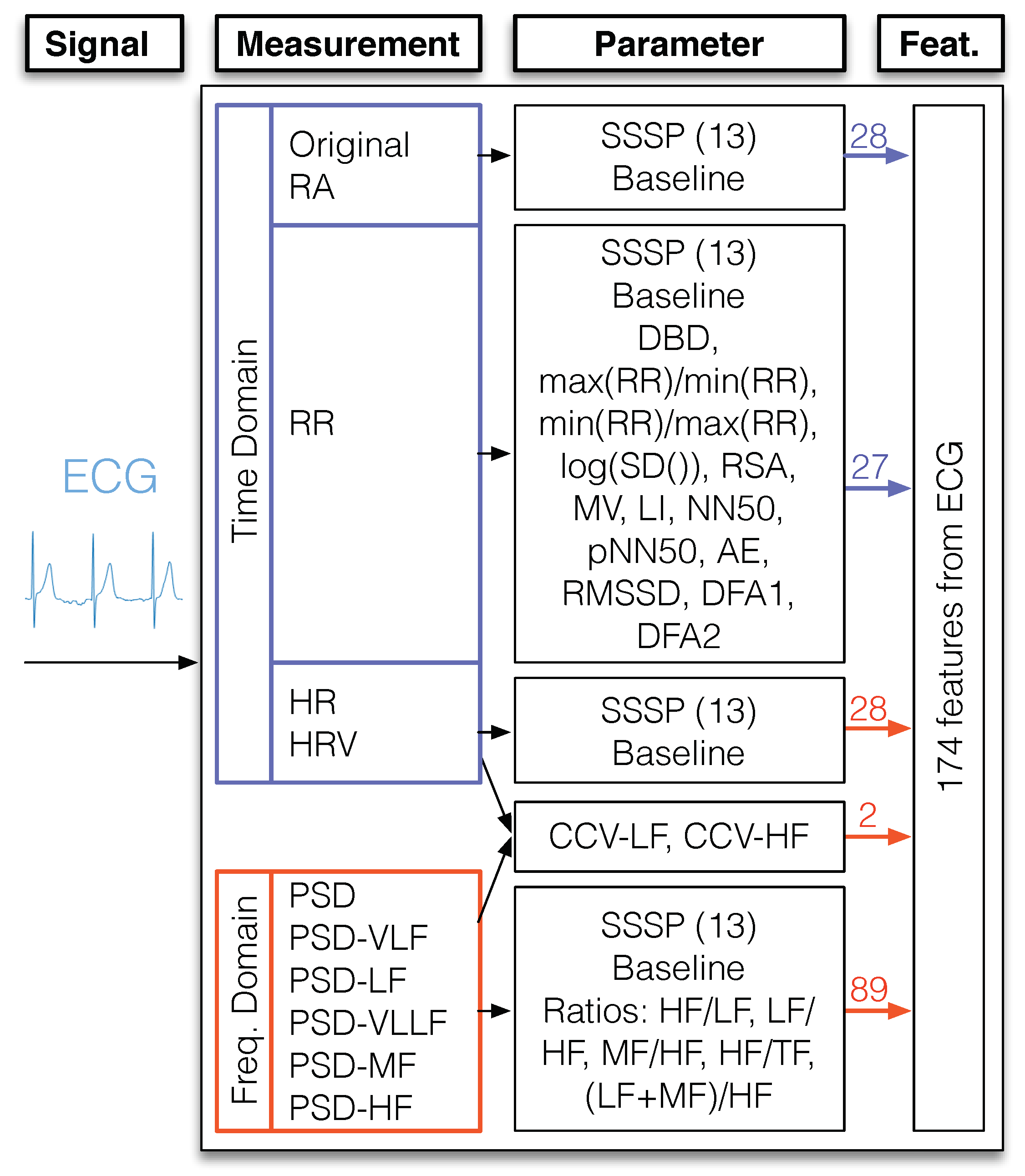
- In our study, we have studied a large number of features which have been selected from a deep revision of the literature. The most frequently used with ECG signals were obtained both in the frequency domain and the time domain: frequency bands [23,26,34,36,37,38,39,40,41,42,43,44,45,46,47,48], and power ratios [23,43,44,46,47,49], in frequency domain; and Heart Rate Variability (HRV) [23,26,38,39,41,42,45,48,50,51], the SDNN [42,48,49], Number of NNs in 50 ms (NN50), pNN50 [34,42,48] and some statistical parameters, such as mean amplitude rate, mean frequency, standard deviations of the raw signals, [25,37,52,53,54,55]. In our study, we have studied all the features found in a literature review of more than 90 papers.The features extracted from the TEB signal are used in some works such as, [24] where the approach is to study cardiovascular reactivity during emotional activation in men and women. Here, the TEB has been acquired together with ECG and the heart sound. In [56] the full respiratory signal was derived from the thoracic impedance raw data, like in our case.
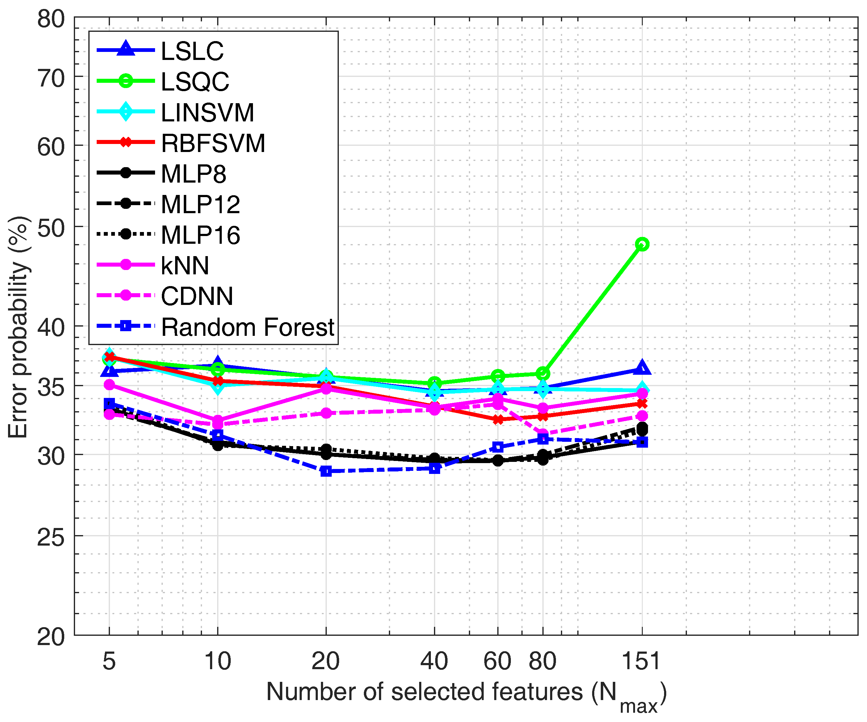
- Most published papers use the calculated features to feed the classifier. Therefore, the number of features used depends on the particular study. We propose to implement feature selection from all the available features to find the best ones and to avoid generalization problems in classification.
- The classifier is usually determined by the author without comparisons or detailed studies about suitability. In numerous works, the selected classifier is the Support Vector Machine (SVM). We think it is positive to make a comparison of different classifiers with very different characteristics.
3. Materials
- Neutral activity, registered during the last 140 s of the first movie (the documentary). As each individual watched each movie twice, there are 280 s for each individual in the database.
- Emotional activity, registered during the viewing of the last 70 s of the second and third movies (140 s); therefore, we obtained a total of 280 s per individual.
- Mental activity, registered during the last 140 s of both games, producing 280 s in total.
- Physical activity registered during the last 280 s of the physical activity stage. To elicit physical load the participant had to go up and down the stairs for five minutes.
4. Methods
4.1. Feature Extraction
4.2. Classification
4.2.1. Least Squares Linear Classifier (LSLC)
4.2.2. Least Squares Quadratic Classifier (LSQC)
4.2.3. Support Vector Machines (SVMs)
4.2.4. Multi-Layer Perceptrons (MLPs)
4.2.5. k-Nearest Neighbor (kNN)
4.2.6. Centroid Displacement-Based k-Nearest Neighborgs (CDNN)
4.2.7. Random Forests (RFs)
4.3. Feature Selection
- A “population” of 100 combinations of features (chromosomes) is randomly generated.
- If there are two combinations with exactly the same set of features, one of them is modified by randomly replacing one of the features.
- For each combination in the population, if the number of features is greater than the maximum , then features are randomly removed from the chromosome until the condition is satisfied.
- Each combination is ranked using the mean squared error of a LSLC measured using the design set.
- The best 10 combinations of the population are selected as “parents” that survive and are used to regenerate the remaining 90 chromosomes using a random crossover of the parents.
- Mutations are added to the population by changing a feature with a probability of 1%. It is important to highlight that the best individual of each population remains unaltered. The process iterates in Step 2 until a given number of generations are evaluated.
- A small value of p-value (typically ) implies that the test suggests that the observed data is inconsistent with the null hypothesis, so the null hypothesis must be rejected.
- The hypothesis is not rejected when the p-value is greater than 0.05. This does not imply that the null hypothesis should be accepted, but that it is feasible.
5. Results and Analysis
5.1. Window Length Selection
5.2. Classifier Selection
5.3. Frequently Selected Features
- From the ECG signal: the geometric mean of the HRV, the mean baseline of the RR, the logarithm of the SD of the RR, and the DFA1 of the HR.
- From the TEB signal: the average BR of the RF, the mean baseline of the BRV, and the minimum of the BRV.
- From the EDA measured in the hand: the mean baseline of the original measurement, and the mean baseline of the processed measurement.
- There are no features from the EDA measured in the hand which is used more than 40% of cases in the case of considering all possible biosignals in the GA. The most frequent one from this signal is the skewness of the processed measurement.
6. Discussion and Conclusion
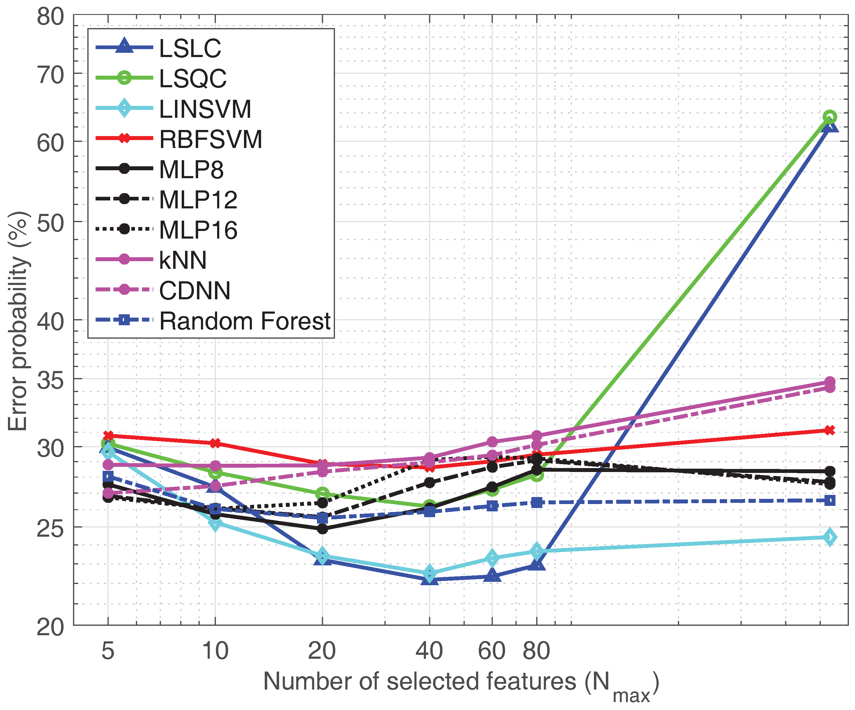
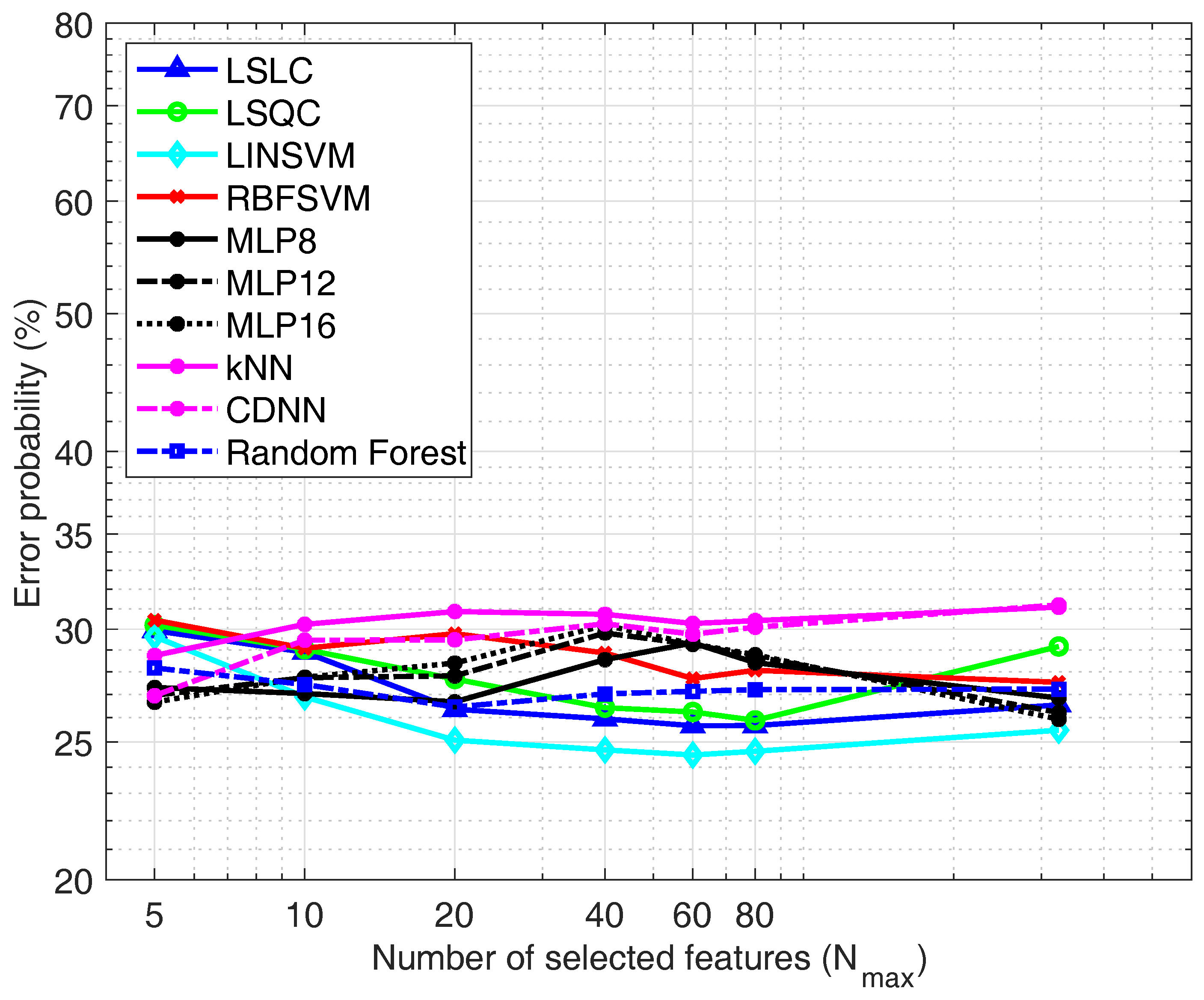
- In most of the relevant cases, the best results are obtained with a window length of 40 s. For the used database, the classifier that render the best results is the simplest ones, the LSLCs.
- When evaluating the combination of physiological signals which is better to correctly detect the type of activity, an LSLC trained with the feature set obtained when applying a GA considering all signals (TEB+ECG+EDA) achieves the lowest classification error probability (22.2%). In the case of the system trained with features selected from the ECG+TEB signal, the results are quite similar (24.5%), and there is no need to measure the EDA signal, making this choice very convenient for those cases in which we desire to pay attention to the simplicity of the acquisition system. That is, the comfort of the subject when there is no need to wear any glove or armband is higher, and the performance of the activity detection system is near the same.
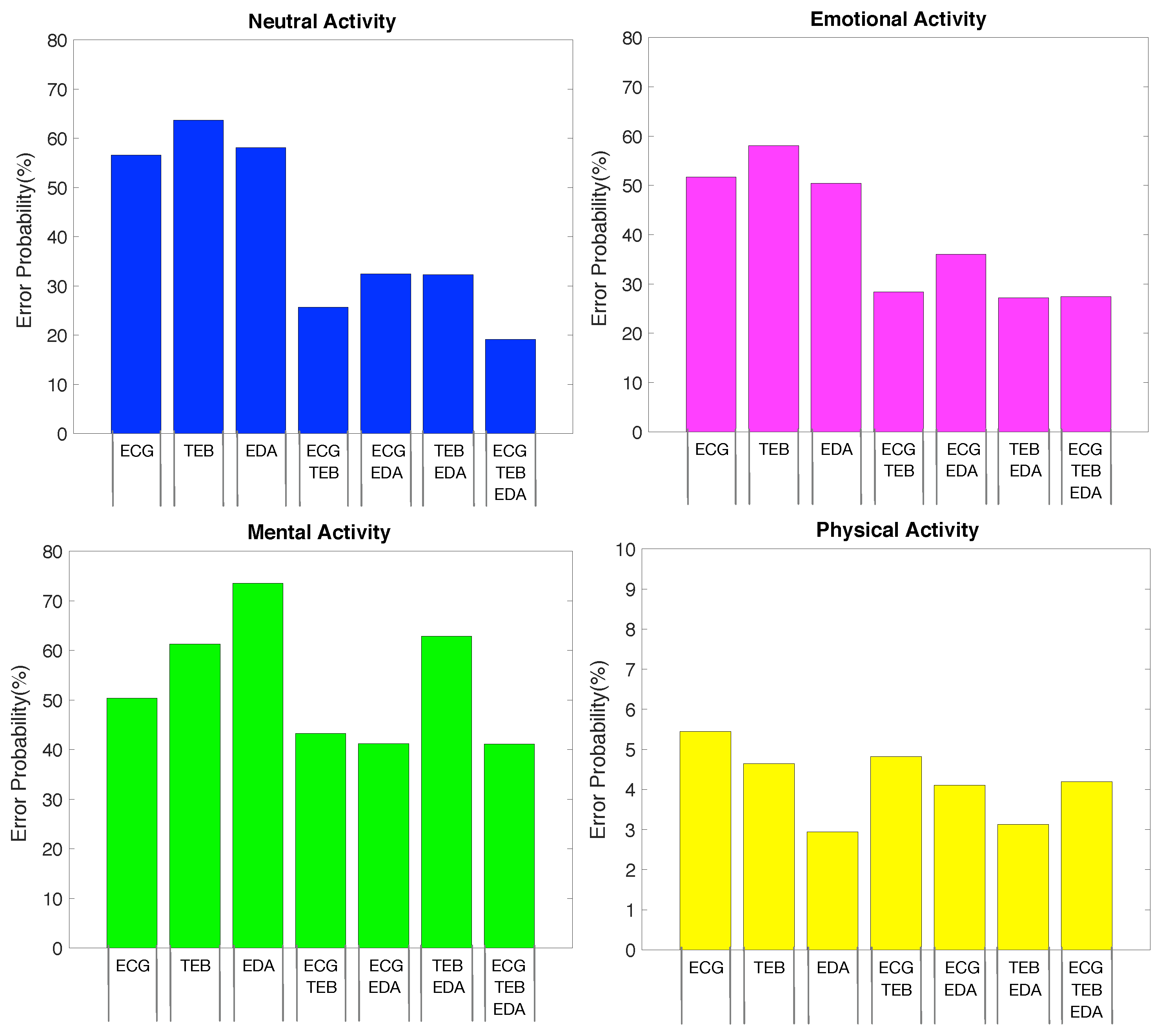
- In addition, for each activity separately the feature set that provides the best results depends significantly on the activity under study. While for neutral activity and mental activity, the best result is obtained with ECG+TEB+EDA feature set, for emotional activity, the best result is obtained with TEB+EDA. Finally, the best result for physical activity is provided by the EDA feature set. This may be because the physical activity causes the activation of the sweat glands in a more meaningful way than the rest of the activities studied. In general, the signals working independently obtain worse results that when we make combinations between signals. Although it depends on the activity under study since in the case of physical activity the results are very similar using one or several signals. However, this does not happen in other cases in which the error is reduced in a remarkable way when combinations of signals are used in the training of the classifier. For the other type of activities, combining sensing modes provides similar or better performance than using only one type of sensing mode.
- The GA seems to be very useful in order to select the most relevant features, improving the results in terms of both complexity after training and error rate. From a total of 533 features, only 40 were necessary to achieve the minimum observed error. TEB signal seems to contain more useful information than the other signals.
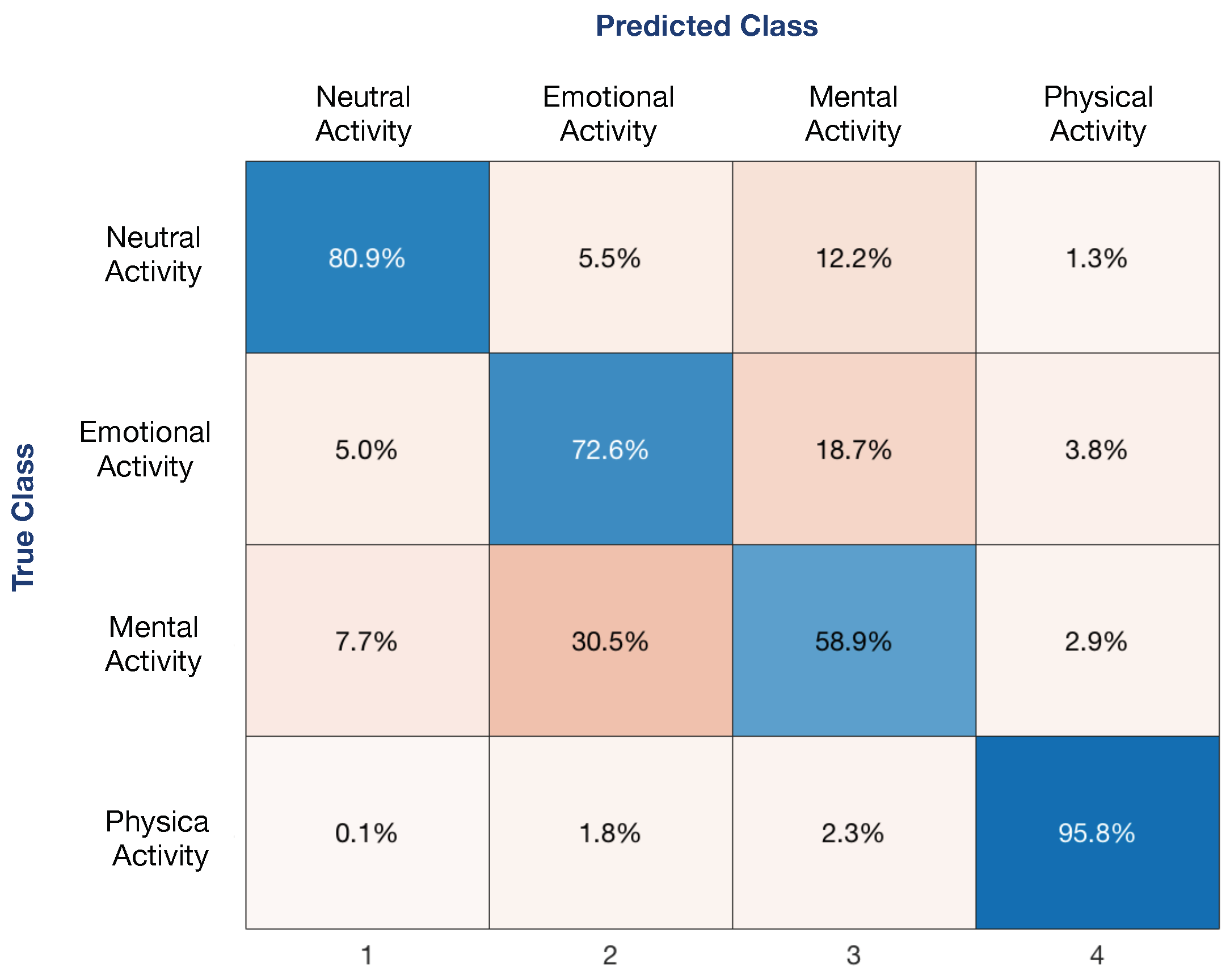
- The results clearly suggest that the activity most easily identifiable is physical activity. Then the neutral, the emotional and finally the mental activity. This is due to the presence of misclassification between emotional and mental activities, as can be naturally expected.
- As a possible limitation of the study, we should consider that these conclusions might be different with other electronic devices. For instance, improvement on the textile based sensors or the use of gel-based classical sensors might improve the quality of the acquired signals, changing the usefulness of the measured features. Furthermore, the use of a more extensive database might overcome the generalization problems, allowing to obtain better results with more complex classifiers. In this sense, this paper does not try to propose a close solution but a methodology, and the comparison of the features and signals carried out might be conditioned to the actual textile sensor technology.
Supplementary Materials
Author Contributions
Funding
Conflicts of Interest
Abbreviations
| ECG | Electrocardiogram |
| TEB | Thoracic Electrical Bioimpedance |
| EDA | Electrodermal Activity |
| HRV | Heart Rate Variability |
| SDNN | Standard Deviation of NN intervals |
| SDSD | Standard Deviation of Successive Differences |
| LSLC | Least Squares Linear Classifier |
| LSQC | Least Squares Quadratic Classifier |
| SVM | Support Vector Machine |
| LINSVM | Linear Support Vector Machine |
| RBFSVM | Radial Basis Function Support Vector Machine |
| MLP | Multi-Layer Perceptron |
| kNN | k-Nearest Neighbor |
| CDNN | Centroid Displacement-based Nearest Classifier |
| RF | Random Forest |
| GA | Genetic Algorithm |
| SSSP | Standard Set of Statistical Parameters |
Appendix A. Features from the ECG Signal

Appendix A.1. Time-Domain
- The interval between successive Rs (RR) (time lapsed between successive R waves) [35,49,80]. Apart from the SSSP and the baseline, some special features have been extracted from the RR measurement:
- –
- –
- Ratios maximum RR vs. minimum RR, that is, RRmax/RRmin and RRmin/RRmax [83].
- –
- Logarithm of the standard deviation of RR in the window under study.
- –
- Respiratory Sinus Arrhythmia (RSA), calculated as the quotient between the DBD and the mean value of the RR in the window under study. This measurement is related to the function of parasympathetic nervous during spontaneous ventilation [84].
- –
- Modal Value (MV), defined as the most frequent value in the RR intervals in the window under study [40].
- –
- Load Index (LI), based on the ratio between the number of occurrences of each Modal Value and DBD [40].
- –
- –
- –
- –
- Root Mean Square of Successive Differences (RMSSD), determined by calculating the square root of the mean squared difference between consecutive RR intervals [34,48,49,87]. The RMSSD is the primary time domain used to estimate the high-frequency beat-to-beat variations that represent vagal regulatory activity [48].
- –
- Heart Rate (HR). It is measured as the number of pulses per unit of time, usually beats per minute (bpm). It is calculated as the inverse of the RR interval. It is obtained through the inverse of the RR interval. This parameter is highly important, as it is related to physical exercise, anxiety, sleep, illness, food intake, and drugs, among others. The increase or decrease on this speed is the answer of our body or mind condition [34,48]. The SSSPs and the baseline parameters were calculated from this measurement.
- Heart Rate Variability (HRV), which has been widely used to extract information about the status of the autonomic nervous system and emotions [23]. The work [88] provides a review of this measurement. In addition, numerous studies reveal the importance of this parameter [23,26,38,39,41,42,45,48,50,51,89]. We decided to obtain the HRV as proposed in [26], where the HRV is determined from a modified version of the HRV sampled at 256 Hz. Once the HRV is obtained, it is possible to extract different valuables features, using the SSSPs and the baseline parameter.
Appendix A.2. Frequency-Domain
- Power per Bands. From this PSD parameter, several frequency bands were considered: Very-Low-frequency (PSD-VLF), taken from 0.0033–0.05 Hz; Low Frequency (PSD-LF) from 0.05–0.08 Hz; Very-Low and Low-Frequency (PSD-VLLF) from 0.0033–0.08 Hz, Mid Frequency (PSD-MF) from 0.08–0.15 Hz. and High frequency (PSD-HF) from 0.15–0.5 Hz. These values were established taking into account several papers such as [23,26,34,36,37,38,40,41,42,43,44,45,46,47,48].
Appendix A.3. Mixed Domain
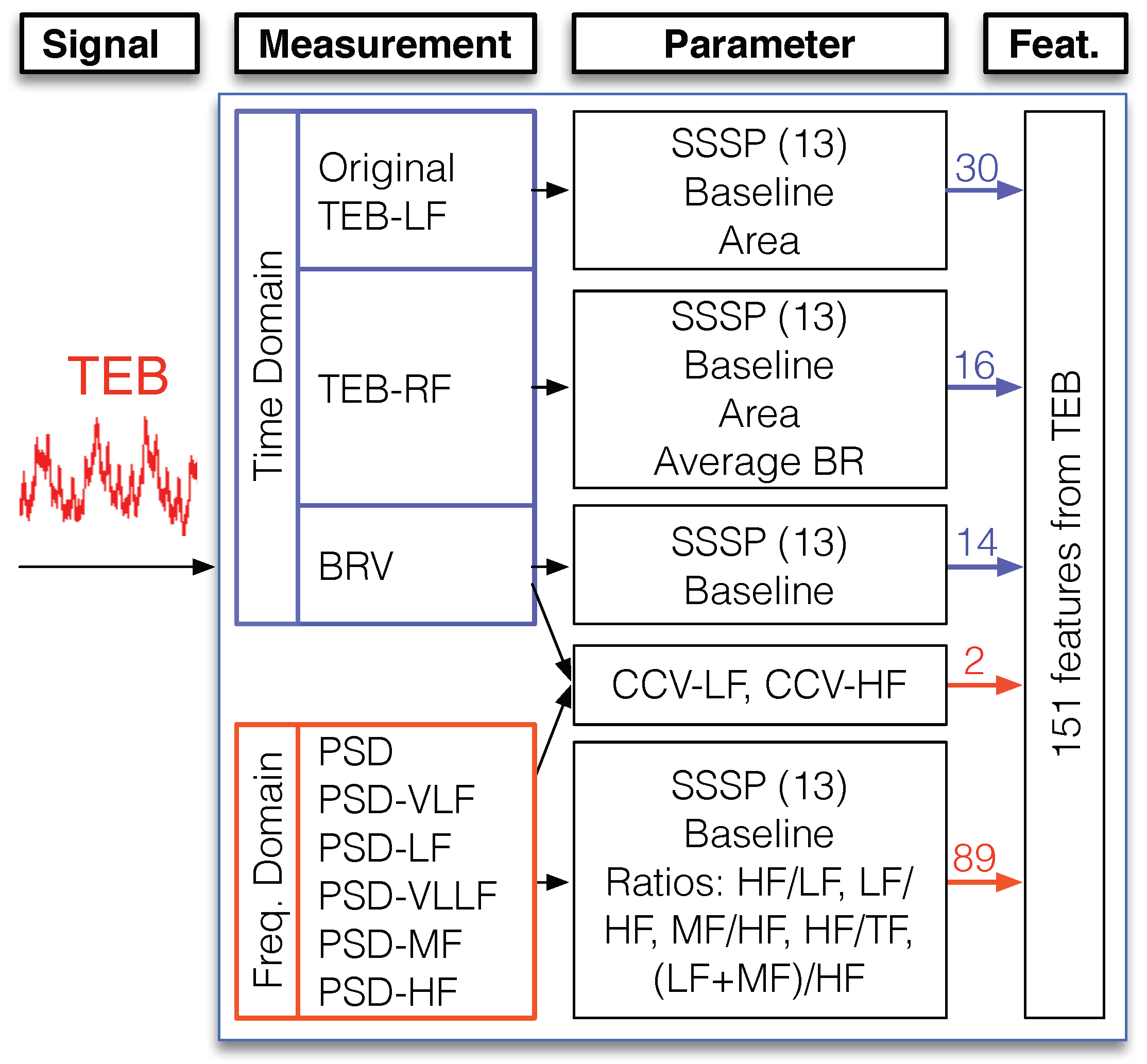
Appendix B. Features from the TEB Signal

Appendix B.1. Time Domain
- TEB-Original Signal: The 13 SSSPs and the baseline parameter aforementioned are calculated from the TEB-Original signal. Apart from these parameters, the area was also calculated, using an approximated segment-based integral of the measurements via a trapezoidal method with unit spacing.
- TEB-LF: the original signal is low-pass filtered (LF block) with a cutoff frequency of 3 Hz, using an FIR filter with order . Again, the 13 SSSPs and the baseline parameter are calculated.
- TEB-RF: Additionally, another new signal is obtained from TEB-LF. The first low pass filter (LF block) acts as an anti-aliasing filter, which allows the use of Interpolated Finite Impulse Response (IFIR) filters [90]. Thus, the output of this anti-aliasing filter is applied to a band-pass filter with cutoff frequencies of 0.1 Hz and 0.5 Hz with a stretch factor of and an order , (being Hz). We denominate TEB Respiration Frequency (TEB-RF) to the measurement obtained. The TEB-RF measurement was used to determine the Breathing Rate (BR). This parameter calculates the number of breaths per minute [91] using a peak detection algorithm. The parameters taken from this measurement, apart from the SSSPs, the baseline, and the area, include the average BR.
- Breath Rate Variability (BRV). Using the BR measured from the TEB-RF, we can calculate the Breath Rate Variability (BRV) in a similar way to HRV. The 13 SSSPs and the baseline parameter are calculated from this measurement.
Appendix B.2. Frequency Domain
Appendix B.3. Mixed Domain
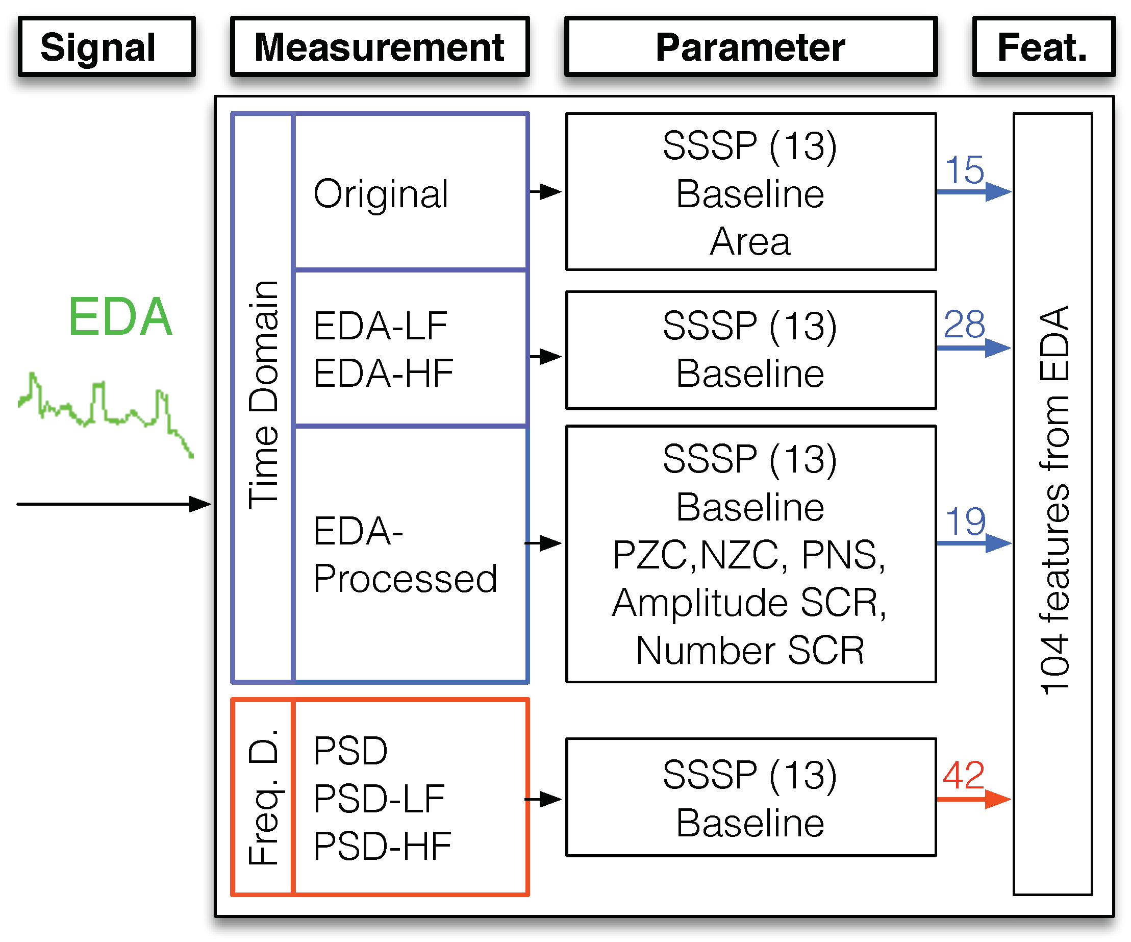
Appendix C. Features from the EDA Signal

Appendix C.1. Time Domain
- EDA-Original Signal. The 13 SSSPs and the baseline aforementioned parameter are calculated to the EDA-Original signal. The area is also calculated from this measurement, using an approximated integral of the time segments through a trapezoidal method with unit spacing.
- EDA-LF: The original signal is filtered with a 20-order low-pass FIR filter (LF block) with a cutoff frequency of 0.2 Hz [41]. The 13 SSSPs and the baseline parameter were evaluated.
- EDA-HF: A complementary filter is also applied to obtain the high frequency components (20-order high-pass FIR filter with a cutoff frequency of 0.2Hz), and the same parameters than those from the EDA-LF measurement are evaluated over the obtained EDA-HF measurement.
- EDA-Processed: The work [26] shows the steps to process EDA signal, for Skin Conductance Response (SCR) detection. The process consists in removing the mean value, resampling to 20 Hz, time differentiating, and filtering with a 20-order Bartlett window. From the processed EDA measurement, typical parameters are extracted using the SSSPs and the baseline parameter, and also some specific parameters:
- –
- –
- Ratio or proportion of Negative Samples (PNS), evaluated as the quotient between the number of negative samples and the total number of samples [41].
- –
- SCRs were evaluated analyzing the zero crossings in the processed EDA signal. The average amplitude of the SCR occurrences and the number of occurrences in the analysis window were used as parameters [26,42,54,91]. SCRs were determined by finding two consecutive zero-crossings, from negative to positive and from positive to negative.
Appendix C.2. Frequency Domain
References
- Rueda, F.M.; Lüdtke, S.; Schröder, M.; Yordanova, K.; Kirste, T.; Fink, G.A. Combining Symbolic Reasoning and Deep Learning for Human Activity Recognition. In Proceedings of the 2019 IEEE International Conference on Pervasive Computing and Communications Workshops (PerCom Workshops), Kyoto, Japan, 11–15 March 2019; pp. 22–27. [Google Scholar]
- Chen, L.M.; Nugent, C.D. Sensor-Based Activity Recognition Review. In Human Activity Recognition and Behaviour Analysis; Springer: Cham, Germany, 2019; pp. 23–47. [Google Scholar]
- Tapia, E.M.; Intille, S.S.; Larson, K. Activity recognition in the home using simple and ubiquitous sensors. In Proceedings of the International Conference on Pervasive Computing, Linz and Vienna, Austria, 21–23 April 2004; pp. 158–175. [Google Scholar]
- Kim, E.; Helal, S.; Cook, D. Human activity recognition and pattern discovery. IEEE Pervasive Comput. 2010, 9, 48–53. [Google Scholar] [CrossRef] [PubMed] [Green Version]
- Bao, L.; Intille, S.S. Activity recognition from user-annotated acceleration data. In Proceedings of the International Conference on Pervasive Computing, Linz and Vienna, Austria, 21–23 April 2004; pp. 1–17. [Google Scholar]
- Handley, T.E.; Lewin, T.J.; Perkins, D.; Kelly, B. Self-recognition of mental health problems in a rural Australian sample. Aust. J. Rural Health 2018, 26, 173–180. [Google Scholar] [CrossRef] [PubMed] [Green Version]
- Del R Millan, J.; Mouriño, J.; Franzé, M.; Cincotti, F.; Varsta, M.; Heikkonen, J.; Babiloni, F. A local neural classifier for the recognition of EEG patterns associated to mental tasks. IEEE Trans. Neural Networks 2002, 13, 678–686. [Google Scholar] [CrossRef] [PubMed] [Green Version]
- Horlings, R.; Datcu, D.; Rothkrantz, L.J. Emotion recognition using brain activity. In Proceedings of the 9th International Conference on Computer Systems and Technologies and Workshop for PhD Students in Computing, Gabrovo, Bulgaria, 12–13 June 2008; p. 6. [Google Scholar]
- Cloete, T.; Scheffer, C. Benchmarking of a full-body inertial motion capture system for clinical gait analysis. In Proceedings of the 2008 30th Annual International Conference of the IEEE Engineering in Medicine and Biology Society, Vancouver, BC, Canada, 20–25 August 2008; pp. 4579–4582. [Google Scholar]
- Fong, D.T.P.; Chan, Y.Y. The use of wearable inertial motion sensors in human lower limb biomechanics studies: A systematic review. Sensors 2010, 10, 11556–11565. [Google Scholar] [CrossRef] [Green Version]
- Kwapisz, J.R.; Weiss, G.M.; Moore, S.A. Activity recognition using cell phone accelerometers. ACM SigKDD Explor. Newsletter 2011, 12, 74–82. [Google Scholar] [CrossRef]
- Mshali, H.; Lemlouma, T.; Moloney, M.; Magoni, D. A survey on health monitoring systems for health smart homes. Int. J. Ind. Ergon. 2018, 66, 26–56. [Google Scholar] [CrossRef] [Green Version]
- Albanie, S.; Nagrani, A.; Vedaldi, A.; Zisserman, A. Emotion Recognition in Speech Using Cross-Modal Transfer in the Wild. Available online: https://arxiv.org/abs/1808.05561 (accessed on 12 December 2019).
- Wang, S.H.; Phillips, P.; Dong, Z.C.; Zhang, Y.D. Intelligent facial emotion recognition based on stationary wavelet entropy and Jaya algorithm. Neurocomputing 2018, 272, 668–676. [Google Scholar] [CrossRef]
- Mohino, I.; Goni, M.; Alvarez, L.; Llerena, C.; Gil-Pita, R. Detection of emotions and stress through speech analysis. In Proceedings of the Signal Processing, Pattern Recognition and Application-2013, Innsbruck, Austria, 12–14 February 2013; pp. 12–14. [Google Scholar]
- Busso, C.; Deng, Z.; Yildirim, S.; Bulut, M.; Lee, C.M.; Kazemzadeh, A.; Lee, S.; Neumann, U.; Narayanan, S. Analysis of emotion recognition using facial expressions, speech and multimodal information. In Proceedings of the 6th International Conference on Multimodal Interfaces, State College, PA, USA, 13–15 October 2004; pp. 205–211. [Google Scholar]
- Lymberis, A.; Olsson, S. Intelligent biomedical clothing for personal health and disease management: State of the art and future vision. Telemed. J. e-Health 2003, 9, 379–386. [Google Scholar] [CrossRef]
- Wei, D.; Nagai, Y.; Jing, L.; Xiao, G. Designing comfortable smart clothing: For infants? health monitoring. Int. J. Des. Creativity Innov. 2019, 7, 116–128. [Google Scholar] [CrossRef]
- Jerritta, S.; Murugappan, M.; Nagarajan, R.; Wan, K. Physiological signals based human emotion recognition: A review. In Proceedings of the 2011 IEEE 7th International Colloquium on Signal Processing and its Applications, Penang, Malaysia, 4–6 March 2011; pp. 410–415. [Google Scholar]
- Agrafioti, F.; Hatzinakos, D.; Anderson, A.K. ECG pattern analysis for emotion detection. IEEE Trans. Affective Comput. 2012, 3, 102–115. [Google Scholar] [CrossRef]
- Rattanyu, K.; Mizukawa, M. Emotion recognition based on ECG signals for service robots in the intelligent space during daily life. J. Adv. Comput. Intell. Intell. Inf. 2011, 15, 582–591. [Google Scholar] [CrossRef]
- Lara, O.D.; Labrador, M.A. A survey on human activity recognition using wearable sensors. IEEE Commun. Surv. Tutor. 2013, 15, 1192–1209. [Google Scholar] [CrossRef]
- McCraty, R.; Atkinson, M.; Tiller, W.A.; Rein, G.; Watkins, A.D. The effects of emotions on short-term power spectrum analysis of heart rate variability. Am. J. Cardiol. 1995, 76, 1089–1093. [Google Scholar] [CrossRef]
- Neumann, S.A.; Waldstein, S.R. Similar patterns of cardiovascular response during emotional activation as a function of affective valence and arousal and gender. J. Psychosomatic Res. 2001, 50, 245–253. [Google Scholar] [CrossRef]
- Mohino-Herranz, I.; Gil-Pita, R.; Ferreira, J.; Rosa-Zurera, M.; Seoane, F. Assessment of mental, emotional and physical stress through analysis of physiological signals using smartphones. Sensors 2015, 15, 25607–25627. [Google Scholar] [CrossRef] [PubMed]
- Kim, K.H.; Bang, S.; Kim, S. Emotion recognition system using short-term monitoring of physiological signals. Med. Biol. Eng. Comput. 2004, 42, 419–427. [Google Scholar] [CrossRef]
- Prokasy, W. Electrodermal Activity in Psychological Research; Elsevier: Amsterdam, The Netherlands, 2012. [Google Scholar]
- Drachen, A.; Nacke, L.E.; Yannakakis, G.; Pedersen, A.L. Correlation between heart rate, electrodermal activity and player experience in first-person shooter games. In Proceedings of the 5th ACM SIGGRAPH Symposium on Video Games, Los Angeles, CA, USA, 28–29 July 2010; pp. 49–54. [Google Scholar]
- Naveteur, J.; Baque, E.F.I. Individual differences in electrodermal activity as a function of subjects’ anxiety. Person. Ind. Differ. 1987, 8, 615–626. [Google Scholar] [CrossRef]
- Bellman, R. Dynamic Programming; Princeton University Press: Princeton, NJ, USA, 1957. [Google Scholar]
- Myers, K.A.; Bello-Espinosa, L.E.; Symonds, J.D.; Zuberi, S.M.; Clegg, R.; Sadleir, L.G.; Buchhalter, J.; Scheffer, I.E. Heart rate variability in epilepsy: A potential biomarker of sudden unexpected death in epilepsy risk. Epilepsia 2018, 59, 1372–1380. [Google Scholar] [CrossRef] [Green Version]
- Cai, J.; Liu, G.; Hao, M. The research on emotion recognition from ECG signal. In Proceedings of the 2009 International Conference on Information Technology and Computer Science, Kiev, Ukraine, 25–26 July 2009; pp. 497–500. [Google Scholar]
- Rumpa, L.D.; Wibawa, A.D.; Attamimi, M.; Sampelawang, P.; Purnomo, M.H.; Palelleng, S. Analysis on Human Heart Signal during Sad Video Stimuli using Heart Rate Variability Triangular Index (HRVi). In Proceedings of the 2018 International Conference on Computer Engineering, Network and Intelligent Multimedia (CENIM), Surabaya, Indonesia, 26–27 November 2018; pp. 25–28. [Google Scholar]
- Malik, M.; Bigger, J.T.; Camm, A.J.; Kleiger, R.E.; Malliani, A.; Moss, A.J.; Schwartz, P.J. Heart rate variability: Standards of measurement, physiological interpretation, and clinical use. Eur. Heart J. 1996, 17, 354–381. [Google Scholar] [CrossRef] [Green Version]
- Cripps, T.; Malik, M.; Farrell, T.; Camm, A. Prognostic value of reduced heart rate variability after myocardial infarction: Clinical evaluation of a new analysis method. Br. Heart J. 1991, 65, 14–19. [Google Scholar] [CrossRef] [Green Version]
- Healey, J.A.; Picard, R.W. Detecting stress during real-world driving tasks using physiological sensors. IEEE Trans. Intell. Transp. Syst. 2005, 6, 156–166. [Google Scholar] [CrossRef] [Green Version]
- Picard, W.; Healey, J.A. Wearable and Automotive Systems for Affect Recognition from Physiology. Available online: http://citeseerx.ist.psu.edu/viewdoc/summary?doi=10.1.1.30.1519 (accessed on 11 December 2019).
- Dishman, R.K.; Nakamura, Y.; Garcia, M.E.; Thompson, R.W.; Dunn, A.L.; Blair, S.N. Heart rate variability, trait anxiety, and perceived stress among physically fit men and women. Int. J. Psychophysiol. 2000, 37, 121–133. [Google Scholar] [CrossRef]
- Vuksanović, V.; Gal, V. Heart rate variability in mental stress aloud. Med. Eng. Phys. 2007, 29, 344–349. [Google Scholar] [CrossRef] [PubMed]
- Tkacz, E.; Komorowski, D. An examination of some heart rate variability analysis indicators in the case of children. In Proceedings of the 15th Annual International Conference of the IEEE Engineering in Medicine and Biology Societ, San Diego, CA, USA, 31 October 1993; pp. 794–795. [Google Scholar]
- Soleymani, M.; Lichtenauer, J.; Pun, T.; Pantic, M. A multimodal database for affect recognition and implicit tagging. IEEE Trans. Affect. Comput. 2012, 3, 42–55. [Google Scholar] [CrossRef] [Green Version]
- Kim, J.; André, E. Emotion recognition based on physiological changes in music listening. IEEE Trans. Pattern Anal. Mach. Intell. 2008, 30, 2067–2083. [Google Scholar] [CrossRef]
- Billman, G.E. The LF/HF ratio does not accurately measure cardiac sympatho-vagal balance. Front. Physiol. 2013, 4, 26. [Google Scholar] [CrossRef] [Green Version]
- Piccirillo, G.; Vetta, F.; Fimognari, F.; Ronzoni, S.; Lama, J.; Cacciafesta, M.; Marigliano, V. Power spectral analysis of heart rate variability in obese subjects: Evidence of decreased cardiac sympathetic responsiveness. Int. J. Obes. Relat. Metab. Disord. 1996, 20, 825–829. [Google Scholar]
- Malarvili, M.; Rankine, L.; Mesbah, M.; Colditz, P.; Boashash, B. Heart rate variability characterization using a time-frequency based instantaneous frequency estimation technique. In Proceedings of the 3rd Kuala Lumpur International Conference on Biomedical Engineering 2006, Kuala Lumpur, Malaysia, 11–14 December 2006; pp. 455–459. [Google Scholar]
- Longin, E.; Schaible, T.; Lenz, T.; König, S. Short term heart rate variability in healthy neonates: Normative data and physiological observations. Early Hum. Dev. 2005, 81, 663–671. [Google Scholar] [CrossRef]
- Winchell, R.J.; Hoyt, D.B. Spectral analysis of heart rate variability in the ICU: A measure of autonomic function. J. Surg. Res. 1996, 63, 11–16. [Google Scholar] [CrossRef]
- Von Borell, E.; Langbein, J.; Després, G.; Hansen, S.; Leterrier, C.; Marchant-Forde, J.; Marchant-Forde, R.; Minero, M.; Mohr, E.; Prunier, A.; et al. Heart rate variability as a measure of autonomic regulation of cardiac activity for assessing stress and welfare in farm animals—A review. Physiol. Behav. 2007, 92, 293–316. [Google Scholar] [CrossRef]
- Pan, J.; Tompkins, W.J. A real-time QRS detection algorithm. IEEE Trans. Biomed. Eng. 1985, 32, 230–236. [Google Scholar] [CrossRef] [PubMed]
- Haag, A.; Goronzy, S.; Schaich, P.; Williams, J. Emotion recognition using bio-sensors: First steps towards an automatic system. In Proceedings of the Tutorial and Research Workshop on Affective Dialogue Systems, Kloster Irsee, Germany, 14–16 June 2004; pp. 36–48. [Google Scholar]
- Brennan, M.; Palaniswami, M.; Kamen, P. Do existing measures of Poincare plot geometry reflect nonlinear features of heart rate variability? IEEE Trans. Biomed. Eng. 2001, 48, 1342–1347. [Google Scholar] [CrossRef] [PubMed]
- Picard, R.W.; Vyzas, E.; Healey, J. Toward machine emotional intelligence: Analysis of affective physiological state. IEEE Trans. Pattern Anal. Mach. Intell. 2001, 23, 1175–1191. [Google Scholar] [CrossRef] [Green Version]
- Rigas, G.; Katsis, C.D.; Ganiatsas, G.; Fotiadis, D.I. A user independent, biosignal based, emotion recognition method. In Proceedings of the 11th International Conference on User Modeling, Corfu, Greece, 25–29 July 2007; pp. 314–318. [Google Scholar]
- Katsis, C.D.; Katertsidis, N.; Ganiatsas, G.; Fotiadis, D.I. Toward emotion recognition in car-racing drivers: A biosignal processing approach. IEEE Trans. Syst. Man Cybern. Part A Syst. Humans 2008, 38, 502–512. [Google Scholar] [CrossRef]
- Maaoui, C.; Pruski, A.; Abdat, F. Emotion recognition for human-machine communication. In Proceedings of the 2008 IEEE/RSJ International Conference on Intelligent Robots and Systems, Nice, France, 22–26 September 2008; pp. 1210–1215. [Google Scholar]
- Lackner, H.K.; Weiss, E.M.; Hinghofer-Szalkay, H.; Papousek, I. Cardiovascular effects of acute positive emotional arousal. Appl. Psychophysiol. Biofeedback 2014, 39, 9–18. [Google Scholar] [CrossRef] [PubMed]
- Wu, G.; Liu, G.; Hao, M. The analysis of emotion recognition from GSR based on PSO. In Proceedings of the 2010 International Symposium on Intelligence Information Processing and Trusted Computing, Huanggang, China, 28–29 October 2010; pp. 360–363. [Google Scholar]
- Caruelle, D.; Gustafsson, A.; Shams, P.; Lervik-Olsen, L. The use of electrodermal activity (EDA) measurement to understand consumer emotions—A literature review and a call for action. J. Bus. Res. 2019, 104, 146–160. [Google Scholar] [CrossRef]
- Hernandez, J.; Riobo, I.; Rozga, A.; Abowd, G.D.; Picard, R.W. Using electrodermal activity to recognize ease of engagement in children during social interactions. In Proceedings of the 2014 ACM International Joint Conference on Pervasive and Ubiquitous Computing, Seattle, WC, USA, 13–17 September 2014; pp. 307–317. [Google Scholar]
- Seoane, F.; Ferreira, J.; Alvarez, L.; Buendia, R.; Ayllón, D.; Llerena, C.; Gil-Pita, R. Sensorized garments and textrode-enabled measurement instrumentation for ambulatory assessment of the autonomic nervous system response in the atrec project. Sensors 2013, 13, 8997–9015. [Google Scholar] [CrossRef]
- Gross, J.J.; Levenson, R.W. Emotion elicitation using films. Cognit. Emot. 1995, 9, 87–108. [Google Scholar] [CrossRef]
- Merck, M. America First: Naming the Nation in US Film; Routledge: Abingdon, UK, 2007. [Google Scholar]
- Clasen, M. Vampire apocalypse: A biocultural critique of Richard Matheson’s I Am Legend. Philosophy Lit. 2010, 34, 313–328. [Google Scholar] [CrossRef]
- von Jagow, B. Representing the Holocaust, Kertész’s Fatelessness and Benigni’s La vita è bella. In Imre Kertész and Holocaust Literature; Purdue University Press: West Lafayette, IN, USA, 2005; p. 76. [Google Scholar]
- Megías, C.F.; Mateos, J.C.P.; Ribaudi, J.S.; Fernández-Abascal, E.G. Validación española de una batería de películas para inducir emociones. Psicothema 2011, 23, 778–785. [Google Scholar]
- Fenton, H.; Grainger, J.; Castoldi, G.L. Cannibal Holocaust: And the Savage Cinema of Ruggero Deodato; Fab Press: Surrey, UK, 1999. [Google Scholar]
- Denot-Ledunois, S.; Vardon, G.; Perruchet, P.; Gallego, J. The effect of attentional load on the breathing pattern in children. Int. J. Psychophysiol. 1998, 29, 13–21. [Google Scholar] [CrossRef]
- Van Trees, H.L. Detection, Estimation, and Modulation Theory; John Wiley & Sons: Hoboken, NJ, USA, 2004. [Google Scholar]
- Vapnik, V.N.; Vapnik, V. Statistical Learning Theory; Wiley: New York, NY, USA, 1998. [Google Scholar]
- Fix, E.; Hodges, J.L. Discriminatory analysis. Nonparametric discrimination: Consistency properties. Int. Stat. Rev. 1989, 57, 238–247. [Google Scholar] [CrossRef]
- Nguyen, B.P.; Tay, W.L.; Chui, C.K. Robust biometric recognition from palm depth images for gloved hands. IEEE Trans. Hum. Mach. Syst. 2015, 45, 799–804. [Google Scholar] [CrossRef]
- Breiman, L. Random Forests. Mach. Learn. 2001, 45, 5–32. [Google Scholar] [CrossRef] [Green Version]
- Kohavi, R.; John, G.H. Wrappers for feature subset selection. Artif. Intell. 1997, 97, 273–324. [Google Scholar] [CrossRef] [Green Version]
- Holland, J.H. Adaptation in Natural and Artificial Systems: An Introductory Analysis with Applications to Biology, Control, and Artificial Intelligence; The University of Michigan Press: Ann Arbor, MI, USA, 1975. [Google Scholar]
- Golberg, D.E. Genetic algorithms in search, optimization, and machine learning. Addion Wesley 1989, 1989, 102. [Google Scholar]
- Zhuo, L.; Zheng, J.; Li, X.; Wang, F.; Ai, B.; Qian, J. A genetic algorithm based wrapper feature selection method for classification of hyperspectral images using support vector machine. In Proceedings of the Geoinformatics 2008 and Joint Conference on GIS and Built Environment: Classification of Remote Sensing Images, Guangzhou, China, 28–29 June 2008; International Society for Optics and Photonics; p. 71471J. [Google Scholar]
- Ferreira, F.L.; Cardoso, S.; Silva, D.; Guerreiro, M.; de Mendonça, A.; Madeira, S.C. Improving Prognostic Prediction from Mild Cognitive Impairment to Alzheimer’s Disease Using Genetic Algorithms. In Proceedings of the 11th International Conference on Practical Applications of Computational Biology & Bioinformatics, Orto, Portugal, 21–23 June 2017; pp. 180–188. [Google Scholar]
- Bautista-Durán, M.; Garía Gómez, J.; Gil-Pita, R.; Mohíno-Herranz, I.; Rosa-Zurera, M. Energy-efficient acoustic violence detector for smart cities. Int. J. Comput. Intell. Syst. 2017, 10, 1298–1305. [Google Scholar]
- Westfall, P.H.; Young, S.S. Resampling-based Multiple Testing: Examples and Methods for P-Value Adjustment; John Wiley & Sons: Hoboken, NI, USA, 1993. [Google Scholar]
- Thuraisingham, R. Preprocessing RR interval time series for heart rate variability analysis and estimates of standard deviation of RR intervals. Comput. Meth. Programs Biomed. 2006, 83, 78–82. [Google Scholar] [CrossRef]
- Ekholm, E.M.; Piha, S.J.; Erkkola, R.U.; Antila, K.J. Autonomic cardiovascular reflexes in pregnancy. A longitudinal study. Clin. Autonomic Res. 1994, 4, 161–165. [Google Scholar] [CrossRef]
- Sathyaprabha, T.; Satishchandra, P.; Netravathi, K.; Sinha, S.; Thennarasu, K.; Raju, T. Cardiac autonomic dysfunctions in chronic refractory epilepsy. Epilepsy Res. 2006, 72, 49–56. [Google Scholar] [CrossRef]
- Sundkvist, G.; O Almér, L.; Lilja, B. Respiratory influence on heart rate in diabetes mellitus. Br. Med. J. 1979, 1, 924. [Google Scholar] [CrossRef] [PubMed] [Green Version]
- Loula, P.; Jäntti, V.; Yli-Hankala, A. Respiratory sinus arrhythmia during anaesthesia: Assessment of respiration related beat-to-beat heart rate variability analysis methods. Int. J. Clin. Monit. Comput. 1997, 14, 241–249. [Google Scholar] [CrossRef] [PubMed]
- Richman, J.S.; Moorman, J.R. Physiological time-series analysis using approximate entropy and sample entropy. Am. J. Physiol. Heart Circul. Physiol. 2000, 278, H2039–H2049. [Google Scholar] [CrossRef] [PubMed] [Green Version]
- Melillo, P.; Bracale, M.; Pecchia, L. Nonlinear Heart Rate Variability features for real-life stress detection. Case study: Students under stress due to university examination. Biomed. Eng. Online 2011, 10, 1. [Google Scholar] [CrossRef] [Green Version]
- Yoo, S.K.; Lee, C.K.; Park, Y.J.; Kim, N.H.; Lee, B.C.; Jeong, K.S. Neural network based emotion estimation using heart rate variability and skin resistance. In Proceedings of the International Conference on Natural Computation, Changsha, China, 27–29 August 2005; pp. 818–824. [Google Scholar]
- Acharya, U.R.; Joseph, K.P.; Kannathal, N.; Lim, C.M.; Suri, J.S. Heart rate variability: A review. Med. Biol. Eng. Comput. 2006, 44, 1031–1051. [Google Scholar] [CrossRef]
- Soleymani, M.; Chanel, G.; Kierkels, J.J.; Pun, T. Affective ranking of movie scenes using physiological signals and content analysis. In Proceedings of the 2nd ACM workshop on Multimedia semantics, British Columbia, BC, Canada, 31 October 2008; pp. 32–39. [Google Scholar]
- Mehrnia, A.; Willson, A.N. On optimal IFIR filter design. In Proceedings of the 2004 IEEE International Symposium on Circuits and Systems (IEEE Cat. No. 04CH37512), Vancouver, BC, Canada, 23–26 May 2004; pp. 3–133. [Google Scholar]
- Hahn, G.; Sipinkova, I.; Baisch, F.; Hellige, G. Changes in the thoracic impedance distribution under different ventilatory conditions. Physiol. Meas 1995, 16, A161. [Google Scholar] [CrossRef]


| Combination of Signals | Par. | Window Length | |||
|---|---|---|---|---|---|
| 10 s | 20 s | 40 s | 60 s | ||
| ECG | Error(%) | 43.0% | 41.2% | 40.1% | 39.6% |
| 174 | 80 | 174 | 80 | ||
| p-value | <0.001 | <0.001 | <0.001 | Best | |
| TEB | Error(%) | 51.0% | 42.2% | 34.6% | 37.8% |
| 60 | 60 | 40 | 20 | ||
| p-value | <0.001 | <0.001 | Best | <0.001 | |
| ECG+TEB+EDA | Error(%) | 26.6% | 27.9% | 22.2% | 24.1% |
| 20 | 80 | 40 | 20 | ||
| p-value | <0.001 | <0.001 | Best | <0.001 | |
| ECG+TEB | Error(%) | 41.9% | 31.3% | 25.7% | 27.1% |
| 80 | 80 | 60 | 40 | ||
| p-value | <0.001 | <0.001 | Best | <0.001 | |
| ECG+EDA | Error(%) | 26.0% | 28.3% | 27.9% | 29.2% |
| 40 | 40 | 40 | 10 | ||
| p-value | Best | <0.001 | <0.001 | <0.001 | |
| TEB+EDA | Error(%) | 29.9% | 31.2% | 29.7% | 30.9% |
| 20 | 20 | 40 | 20 | ||
| p-value | <0.001 | <0.001 | Best | <0.001 | |
| EDA | Error(%) | 36.1% | 37.3% | 36.5% | 37.1% |
| 20 | 20 | 20 | 20 | ||
| p-value | Best | 0.003 | <0.001 | <0.001 | |
| Classifier | Single Signal | Combination of Signals | ||||||||
|---|---|---|---|---|---|---|---|---|---|---|
| ECG | ||||||||||
| ECG | TEB | EDA | EDA | TEB | ECG | ECG | TEB | EDA | ||
| Arm | Hand | EDA | TEB | EDA | EDA | |||||
| LSLC | Error | 40.1 | 34.6 | 45.3 | 39.0 | 22.2 | 25.7 | 27.9 | 29.7 | 36.5 |
| 174 | 40 | 10 | 5 | 40 | 60 | 40 | 40 | 20 | ||
| LSQC | Error | 39.3 | 35.2 | 71.2 | 52.8 | 26.2 | 25.9 | 40.6 | 31.9 | 51.4 |
| 60 | 40 | 5 | 40 | 40 | 80 | 20 | 20 | 20 | ||
| LINSVM | Error | 41.0 | 34.5 | 61.7 | 47.0 | 22.5 | 24.5 | 36.4 | 28.7 | 47.2 |
| 174 | 40 | 104 | 104 | 40 | 60 | 382 | 60 | 208 | ||
| RBFSVM | Error | 43.3 | 32.4 | 61.8 | 53.3 | 28.6 | 27.5 | 41.9 | 35.4 | 55.0 |
| 174 | 60 | 40 | 40 | 40 | 325 | 80 | 20 | 40 | ||
| MLP8 | Error | 41.3 | 29.5 | 61.7 | 43.9 | 24.9 | 26.7 | 35.8 | 29.2 | 46.4 |
| 174 | 40 | 60 | 20 | 20 | 20 | 10 | 20 | 10 | ||
| MLP12 | Error | 41.4 | 29.6 | 61.7 | 44.4 | 25.6 | 26.2 | 37.7 | 30.3 | 46.9 |
| 174 | 60 | 60 | 20 | 20 | 325 | 10 | 20 | 10 | ||
| MLP16 | Error | 41.6 | 29.6 | 61.9 | 45.1 | 26.1 | 25.9 | 38.2 | 30.5 | 47.3 |
| 174 | 60 | 20 | 20 | 10 | 325 | 10 | 10 | 10 | ||
| kNN | Error | 45.6 | 32.4 | 55.4 | 49.0 | 28.7 | 28.7 | 40.3 | 33.1 | 50.5 |
| 174 | 10 | 10 | 20 | 10 | 5 | 5 | 10 | 10 | ||
| CDNN | Error | 44.5 | 31.4 | 54.7 | 47.6 | 27.0 | 26.9 | 38.9 | 31.3 | 49.1 |
| 174 | 80 | 5 | 10 | 5 | 5 | 10 | 20 | 10 | ||
| RF | Error | 41.0 | 28.9 | 54.9 | 50.9 | 25.5 | 26.5 | 36.7 | 28.2 | 46.5 |
| 20 | 20 | 10 | 10 | 20 | 20 | 40 | 80 | 20 | ||
| Single Signal | Combination of Signals | ||||||||
|---|---|---|---|---|---|---|---|---|---|
| ECG | |||||||||
| ECG | TEB | EDA | EDA | TEB | ECG | ECG | TEB | EDA | |
| Signal: Measurement | Arm | Hand | EDA | TEB | EDA | EDA | |||
| ECG: Original | 6.5 | - | - | - | 1.5 | 3.5 | 3.8 | - | - |
| ECG: RR | 13.1 | - | - | - | 4.9 | 8.3 | 6.0 | - | - |
| ECG: RA | 6.7 | - | - | - | 2.4 | 3.5 | 2.2 | - | - |
| ECG: HR | 6.5 | - | - | - | 1.5 | 2.9 | 1.1 | - | - |
| ECG: HRV | 2.8 | - | - | - | 2.4 | 2.4 | 2.2 | - | - |
| ECG: PSD | 0.6 | - | - | - | 0.4 | 0.7 | 0.3 | - | - |
| ECG: PSD-VLF | 0.5 | - | - | - | 0.3 | 0.4 | 0.7 | - | - |
| ECG: PSD-LF | 0.6 | - | - | - | 0.4 | 0.5 | 0.8 | - | - |
| ECG: PSD-MF | 0.9 | - | - | - | 0.4 | 0.6 | 0.9 | - | - |
| ECG: PSD-HF | 1.0 | - | - | - | 0.4 | 0.7 | 0.7 | - | - |
| ECG: PSD-VLLF | 0.6 | - | - | - | 0.3 | 0.4 | 0.7 | - | - |
| TEB: Original | - | 8.4 | - | - | 1.4 | 3.1 | - | 1.6 | - |
| TEB: LF | - | 8.9 | - | - | 1.4 | 3.8 | - | 1.5 | - |
| TEB: RF | - | 10.1 | - | - | 2.0 | 1.2 | - | 3.3 | - |
| TEB: BRV | - | 5.0 | - | - | 2.5 | 3.6 | - | 3.8 | - |
| TEB: PSD | - | 1.9 | - | - | 0.3 | 0.6 | - | 0.2 | - |
| TEB: PSD-VLF | - | 0.9 | - | - | 0.6 | 0.5 | - | 0.7 | - |
| TEB: PSD-LF | - | 0.8 | - | - | 1.0 | 1.0 | - | 1.1 | - |
| TEB: PSD-MF | - | 1.0 | - | - | 1.0 | 0.9 | - | 1.1 | - |
| TEB: PSD-HF | - | 2.3 | - | - | 0.7 | 0.9 | - | 0.6 | - |
| TEB: PSD-VLLF | - | 0.8 | - | - | 0.6 | 0.6 | - | 0.7 | - |
| EDA-arm: Original | - | - | 5.6 | - | 0.6 | - | 1.6 | 1.3 | 2.6 |
| EDA-arm: Processed | - | - | 9.8 | - | 1.3 | - | 2.4 | 2.5 | 3.5 |
| EDA-arm: LF | - | - | 8.9 | - | 0.6 | - | 1.5 | 1.3 | 4.0 |
| EDA-arm: HF | - | - | 7.8 | - | 0.6 | - | 0.8 | 0.8 | 3.8 |
| EDA-arm: PSD | - | - | 3.2 | - | 0.5 | - | 0.9 | 0.7 | 1.4 |
| EDA-arm: PSD-LF | - | - | 1.9 | - | 0.4 | - | 0.4 | 0.7 | 0.5 |
| EDA-arm: PSD-HF | - | - | 2.9 | - | 0.4 | - | 0.8 | 0.6 | 1.3 |
| EDA-hand: Original | - | - | - | 2.8 | 1.9 | - | 1.7 | 2.1 | 2.3 |
| EDA-hand: Processed | - | - | - | 11.6 | 3.9 | - | 6.0 | 6.9 | 9.2 |
| EDA-hand: LF | - | - | - | 6.1 | 1.5 | - | 1.5 | 1.9 | 2.7 |
| EDA-hand: HF | - | - | - | 6.6 | 1.4 | - | 1.7 | 2.0 | 3.2 |
| EDA-hand: PSD | - | - | - | 1.3 | 0.2 | - | 0.4 | 0.7 | 0.8 |
| EDA-hand: PSD-LF | - | - | - | 7.1 | 0.2 | - | 0.6 | 2.4 | 3.1 |
| EDA-hand: PSD-HF | - | - | - | 4.6 | 0.2 | - | 0.4 | 1.2 | 1.6 |
| Feature | Combination of Signals | ||||
|---|---|---|---|---|---|
| ECG | |||||
| TEB | ECG | TEB | |||
| Signal | Measure | Parameter | TEB | EDA | |
| TEB | RF | Average BR | 100% | 0% | 100% |
| TEB | BRV | Mean baseline | 100% | 0% | 100% |
| EDA-hand | Original | Mean baseline | 0% | 100% | 100% |
| EDA-hand | Processed | Mean baseline | 0% | 100% | 100% |
| ECG | HRV | Geom. mean | 0% | 0% | 100% |
| ECG | RR | Mean baseline | 0% | 0% | 100% |
| ECG | RR | log(SD()) | 0% | 0% | 99% |
| ECG | RR | DFA1 | 0% | 0% | 98% |
| TEB | BRV | Minimum | 100% | 0% | 94% |
| ECG | HR | Mean baseline | 0% | 0% | 93% |
| ECG | HRV | Mean baseline | 0% | 0% | 87% |
| ECG | RA | Mean baseline | 0% | 0% | 68% |
| EDA-hand | LF | Mean baseline | 0% | 43% | 56% |
| TEB | PSD-VLLF | Mean baseline | 66% | 0% | 50% |
| TEB | PSD-MF | Mean baseline | 97% | 0% | 50% |
| EDA-hand | Processed | Number SCR | 0% | 100% | 49% |
| EDA-hand | HF | Mean baseline | 0% | 57% | 48% |
| TEB | PSD-VLF | Mean baseline | 72% | 0% | 48% |
| TEB | PSD-LF | Mean baseline | 56% | 0% | 48% |
| ECG | Original | Skewness | 0% | 0% | 44% |
| ECG | RA | Mean abs. dev. | 0% | 0% | 40% |
| EDA-arm | Processed | Skewness | 0% | 8% | 40% |
| TEB | PSD-HF | HF/LF | 78% | 0% | 39% |
| TEB | LF | Mean baseline | 100% | 0% | 37% |
| ECG | RA | SD | 0% | 0% | 36% |
| TEB | Original | Mean baseline | 100% | 0% | 36% |
| ECG | RR | 25% Trm. mean | 0% | 0% | 36% |
| TEB | PSD-LF | (LF+MF)/HF | 25% | 0% | 35% |
| EDA-hand | Processed | PNS | 0% | 35% | 35% |
| EDA-hand | Processed | NZC | 0% | 41% | 34% |
| EDA-hand | Processed | PZC | 0% | 24% | 33% |
| TEB | PSD-MF | MF/HF | 5% | 0% | 33% |
| TEB | RF | Mean baseline | 100% | 0% | 33% |
| TEB | LF | Percentile 75% | 93% | 0% | 32% |
| EDA-hand | Processed | Maximum | 0% | 82% | 31% |
| ECG | RR | Median | 0% | 0% | 31% |
| EDA-hand | Processed | Minimum | 0% | 47% | 27% |
| EDA-hand | Processed | Median | 0% | 100% | 26% |
| ECG | RR | Geom. mean | 0% | 0% | 25% |
| TEB | Original | Percentile 75% | 16% | 0% | 23% |
© 2019 by the authors. Licensee MDPI, Basel, Switzerland. This article is an open access article distributed under the terms and conditions of the Creative Commons Attribution (CC BY) license (http://creativecommons.org/licenses/by/4.0/).
Share and Cite
Mohino-Herranz, I.; Gil-Pita, R.; Rosa-Zurera, M.; Seoane, F. Activity Recognition Using Wearable Physiological Measurements: Selection of Features from a Comprehensive Literature Study. Sensors 2019, 19, 5524. https://doi.org/10.3390/s19245524
Mohino-Herranz I, Gil-Pita R, Rosa-Zurera M, Seoane F. Activity Recognition Using Wearable Physiological Measurements: Selection of Features from a Comprehensive Literature Study. Sensors. 2019; 19(24):5524. https://doi.org/10.3390/s19245524
Chicago/Turabian StyleMohino-Herranz, Inma, Roberto Gil-Pita, Manuel Rosa-Zurera, and Fernando Seoane. 2019. "Activity Recognition Using Wearable Physiological Measurements: Selection of Features from a Comprehensive Literature Study" Sensors 19, no. 24: 5524. https://doi.org/10.3390/s19245524