Comparison of Three Algorithms for the Retrieval of Land Surface Temperature from Landsat 8 Images


Abstract
:1. Introduction
2. Materials and Methods
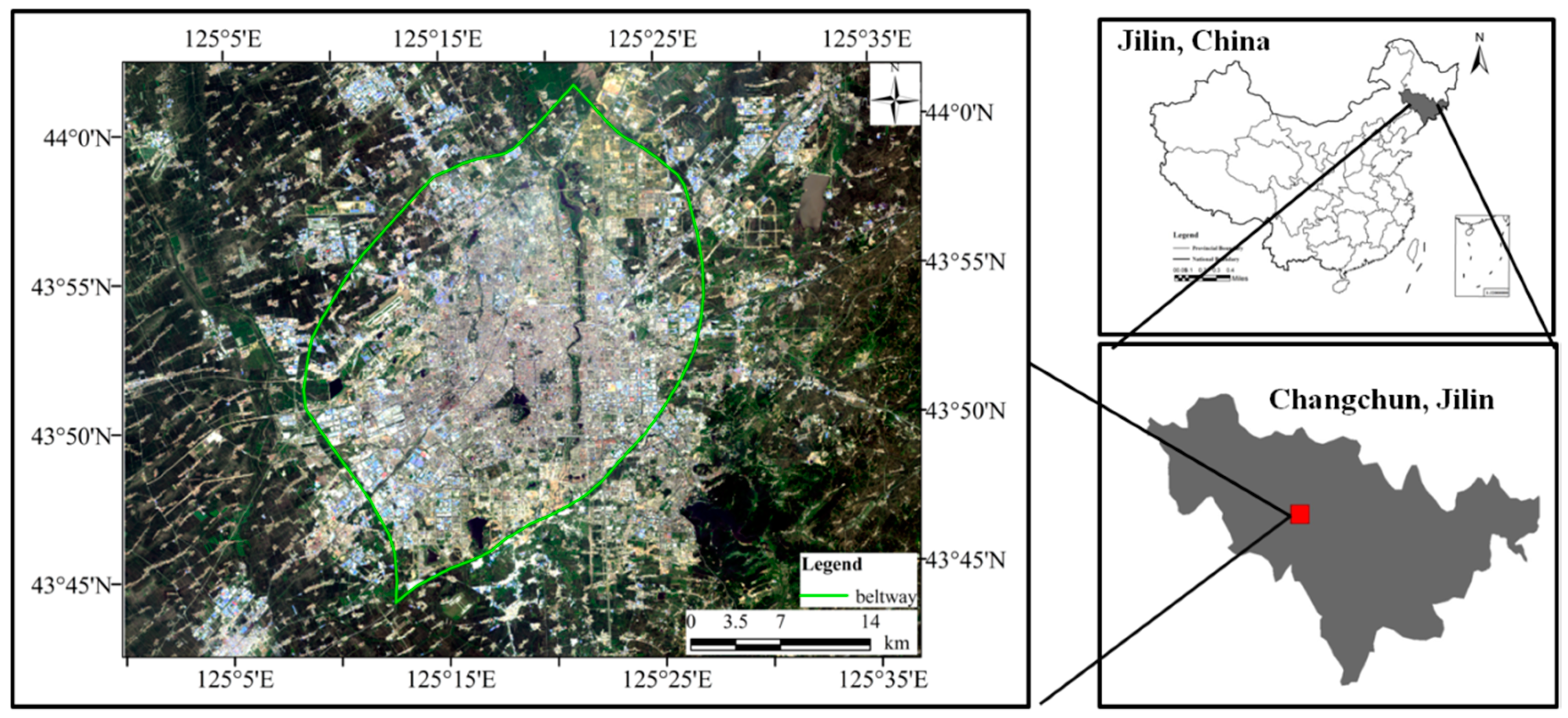
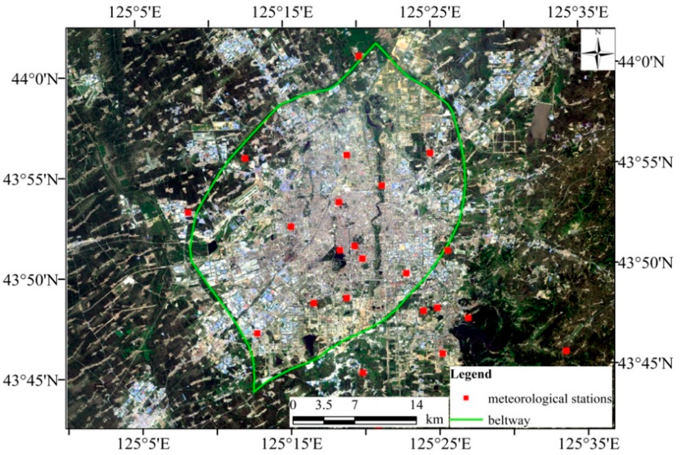
2.1. Study Area
2.2. Data Preprocessing
2.3. Algorithms and Parameter Calculation
2.3.1. Mono-Window Algorithm (MWA)
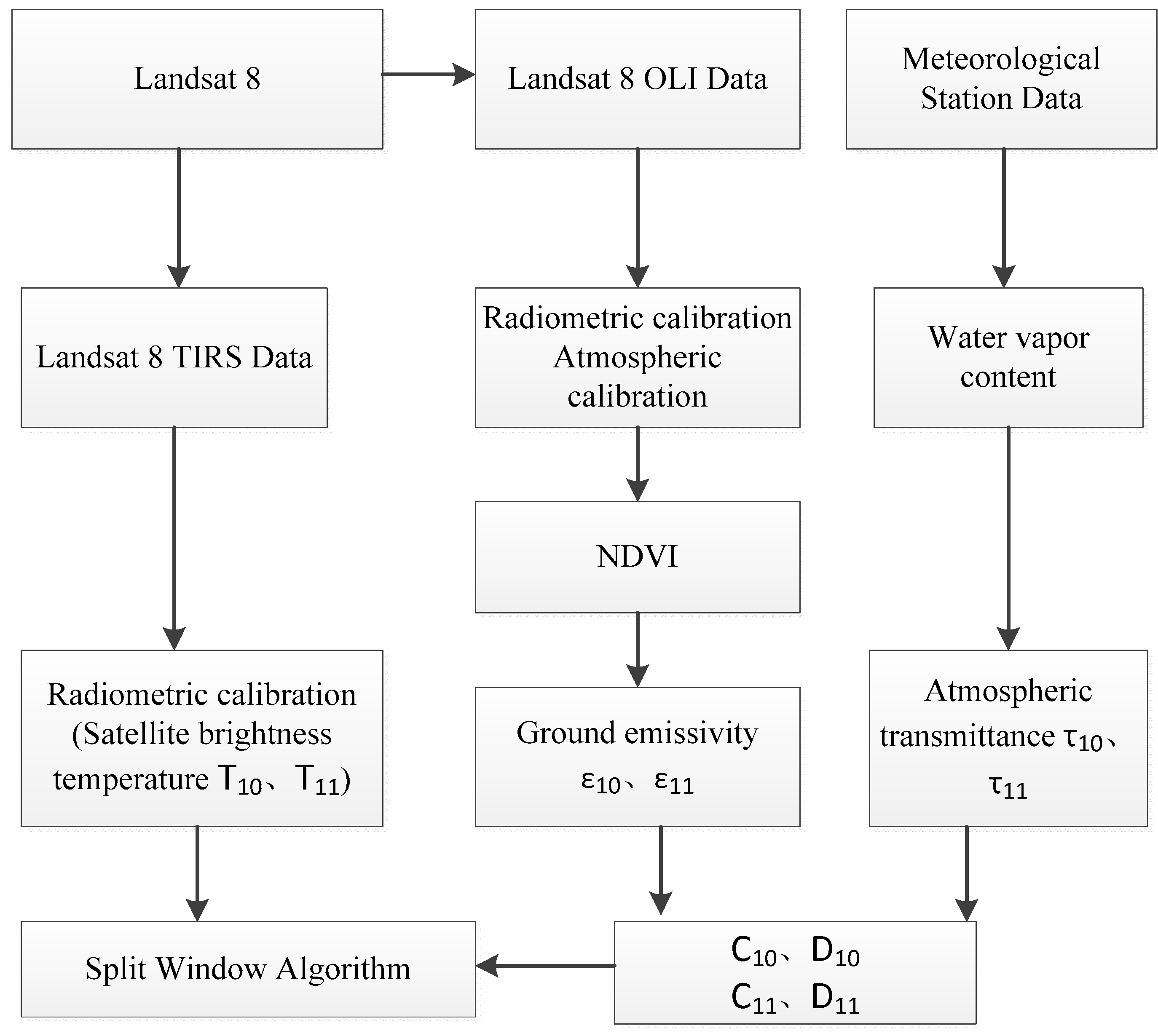
2.3.2. Split Window Algorithm (SWA)
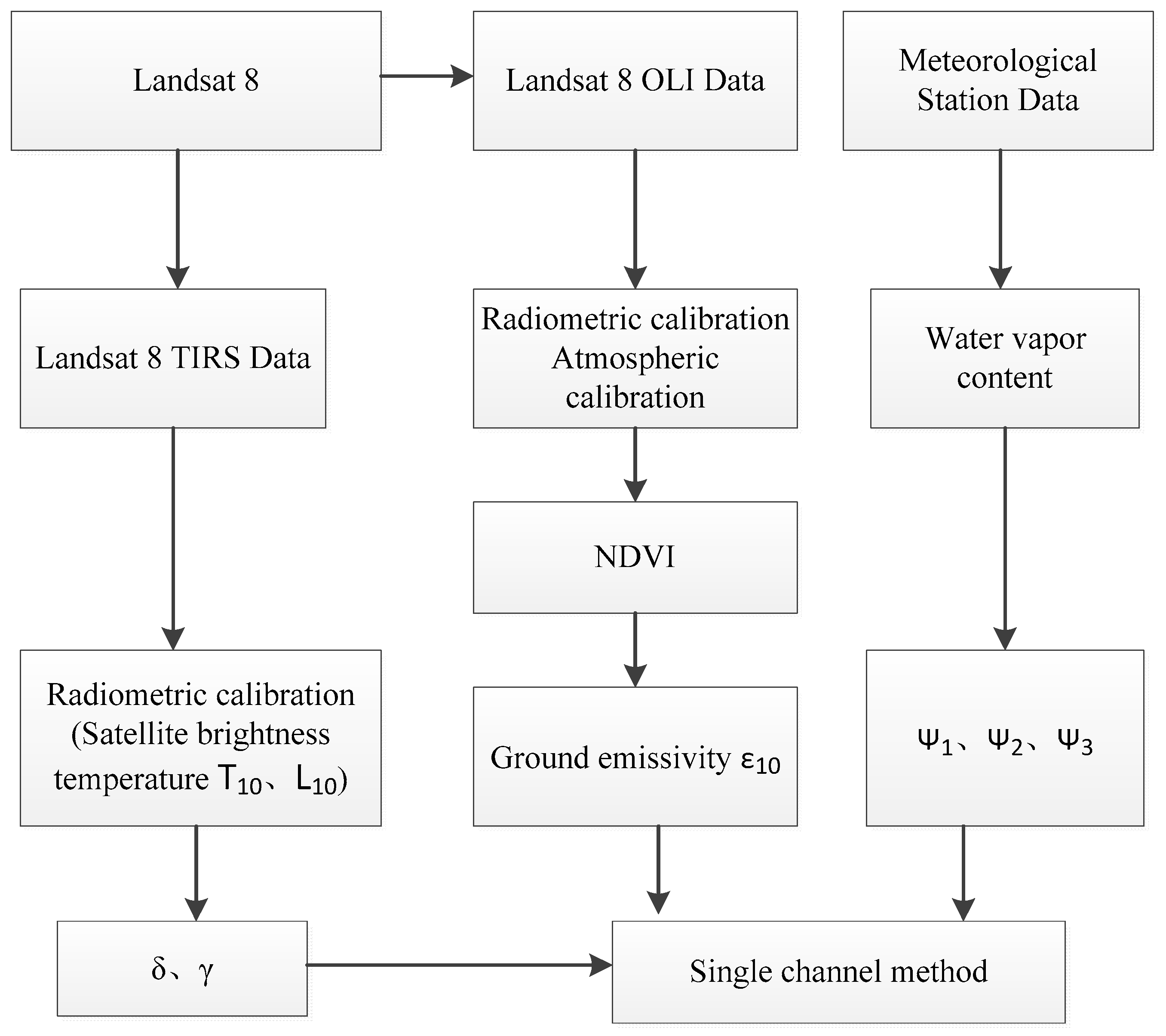
2.3.3. Single-Channel (SC) Method
2.4. Sensitivity Analysis of the Three Algorithms
2.4.1. Sensitivity Analysis of the MWA
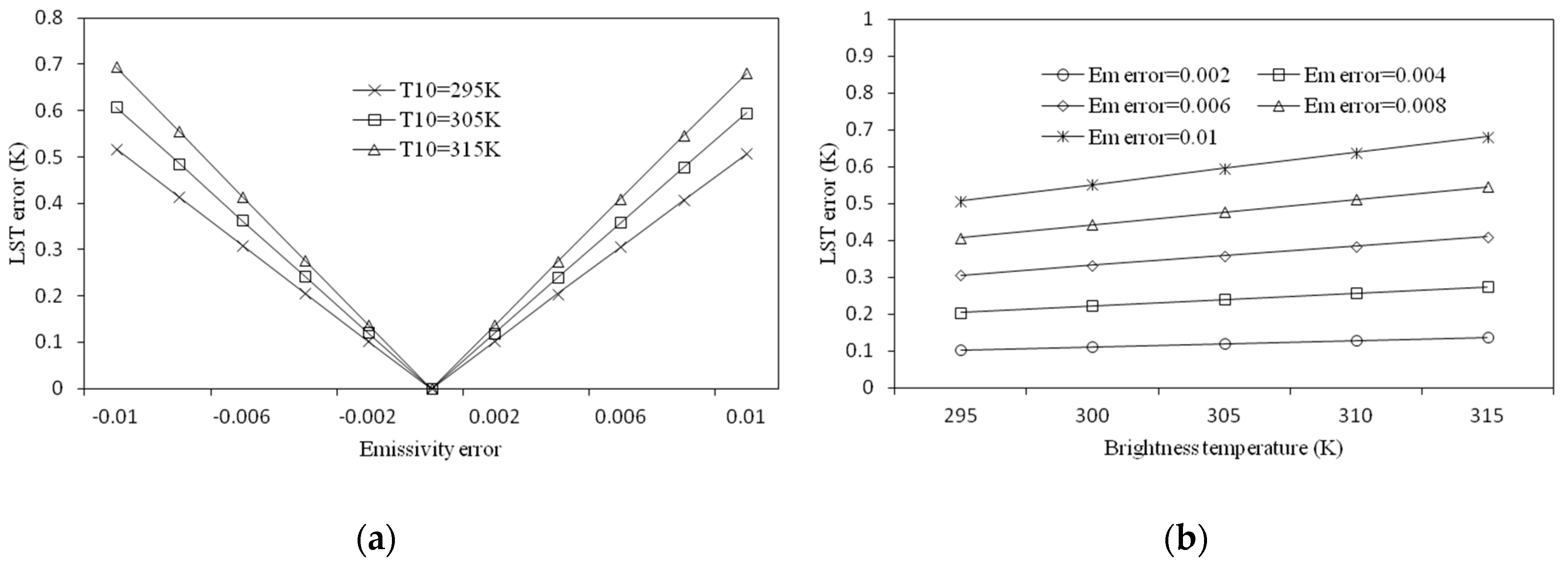
Sensitivity Analysis to LSE
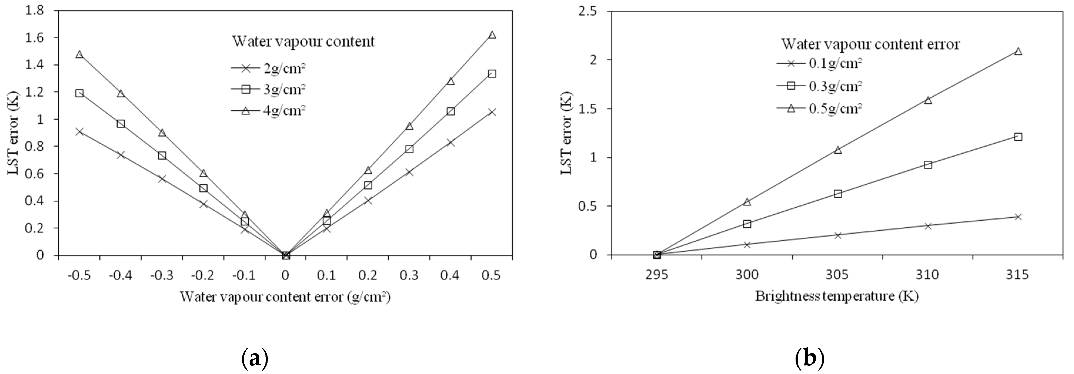
Sensitivity Analysis to Water Vapor Content
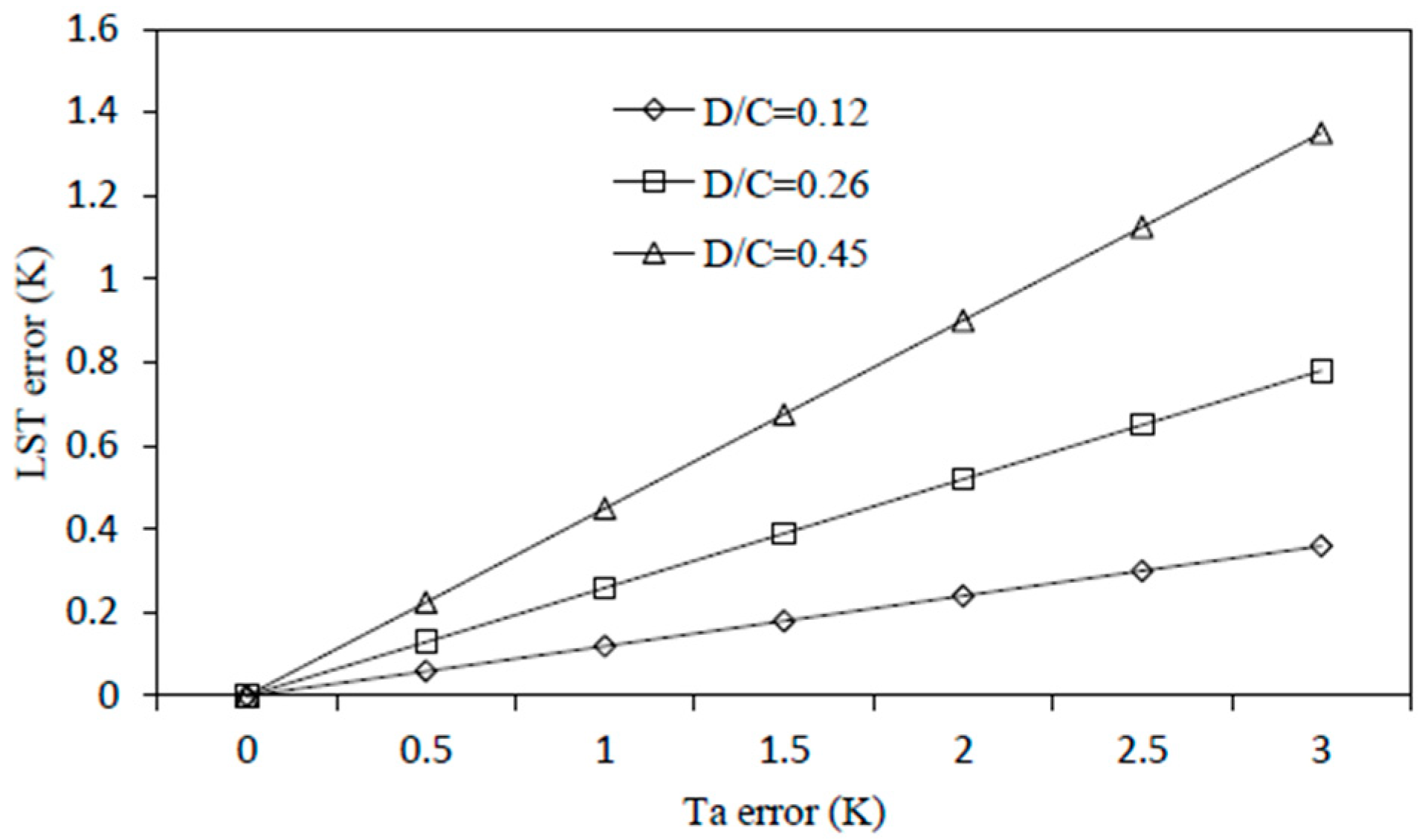
Sensitivity Analysis to Effective Mean Atmosphere Temperature
2.4.2. Sensitivity Analysis of the SWA
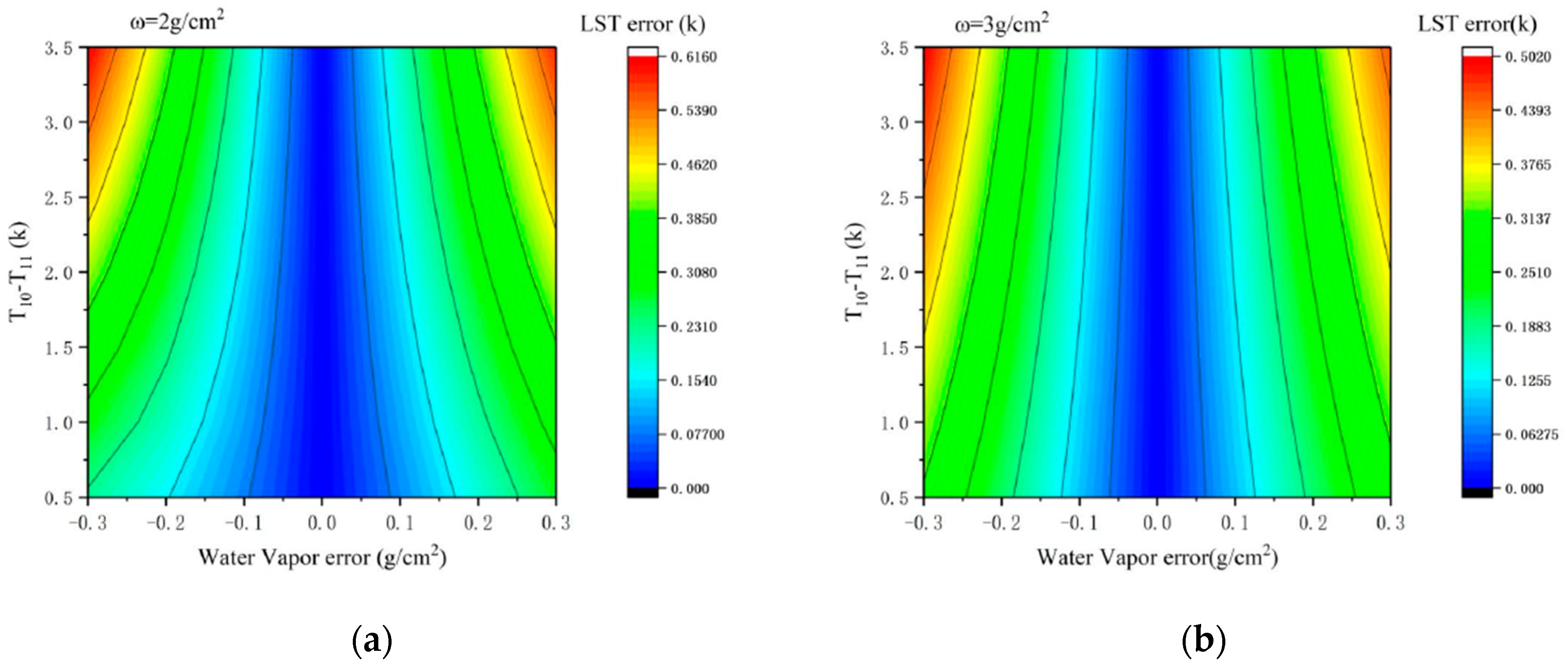
Sensitivity Analysis to the Water Vapor Content
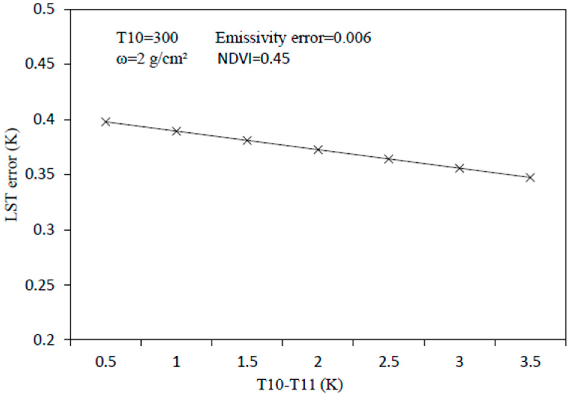
Sensitivity Analysis to the LSE
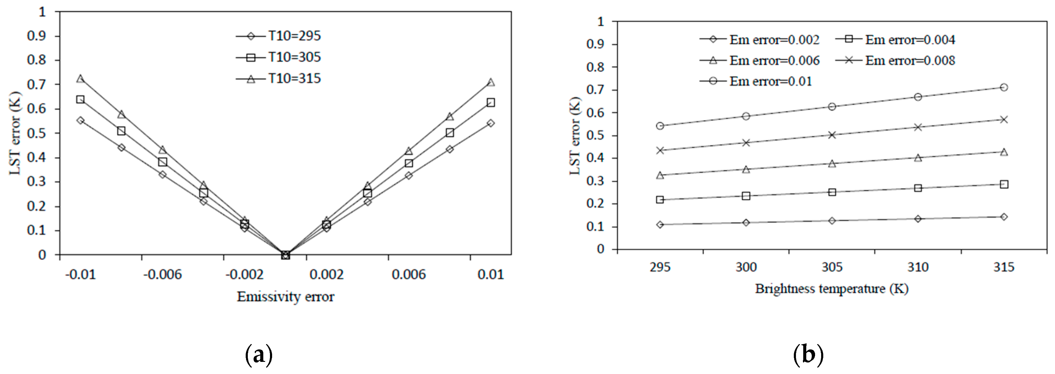
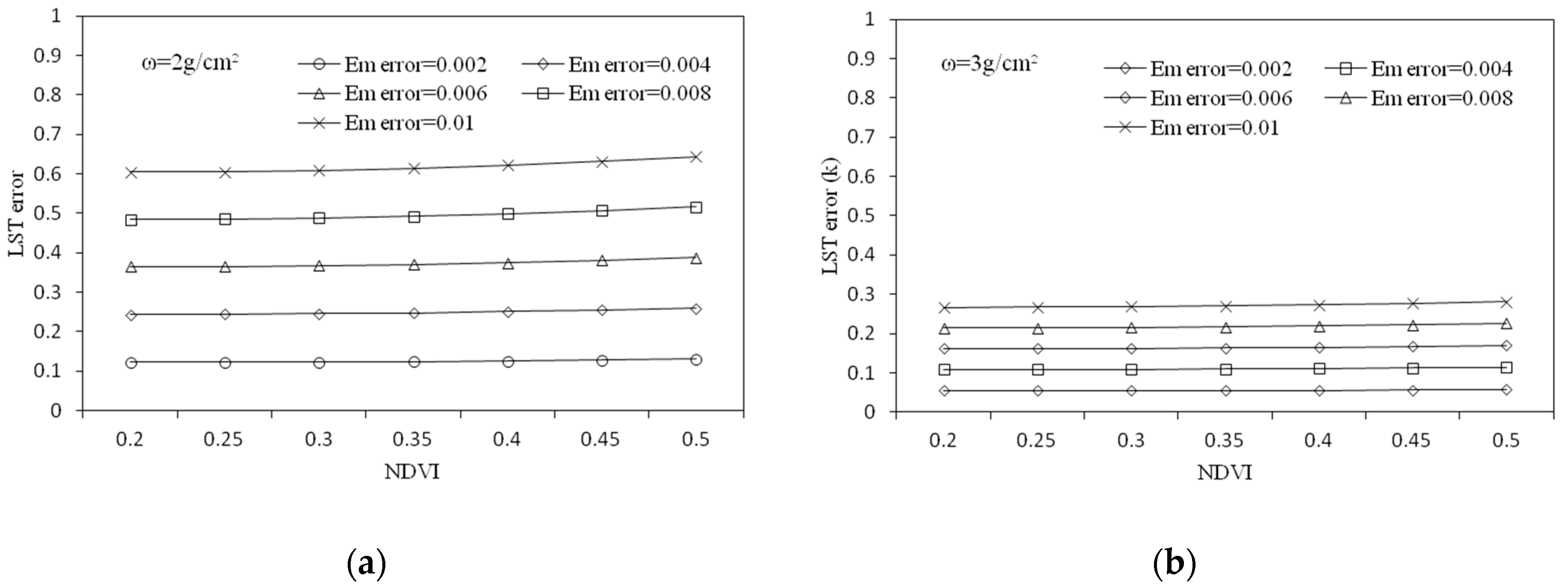
2.4.3. Sensitivity Analysis of the SC Method
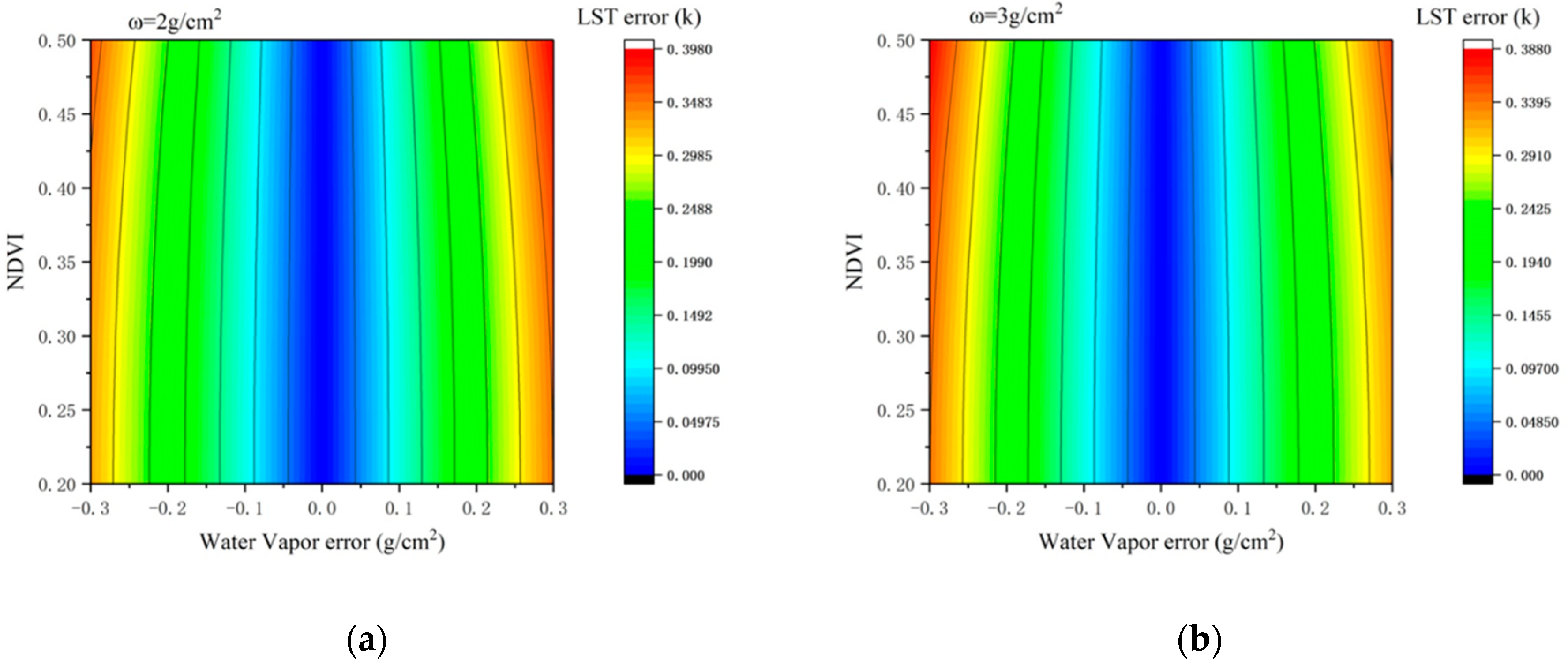
Sensitivity Analysis to Water Vapor Content
Sensitivity Analysis to LSE
3. Results
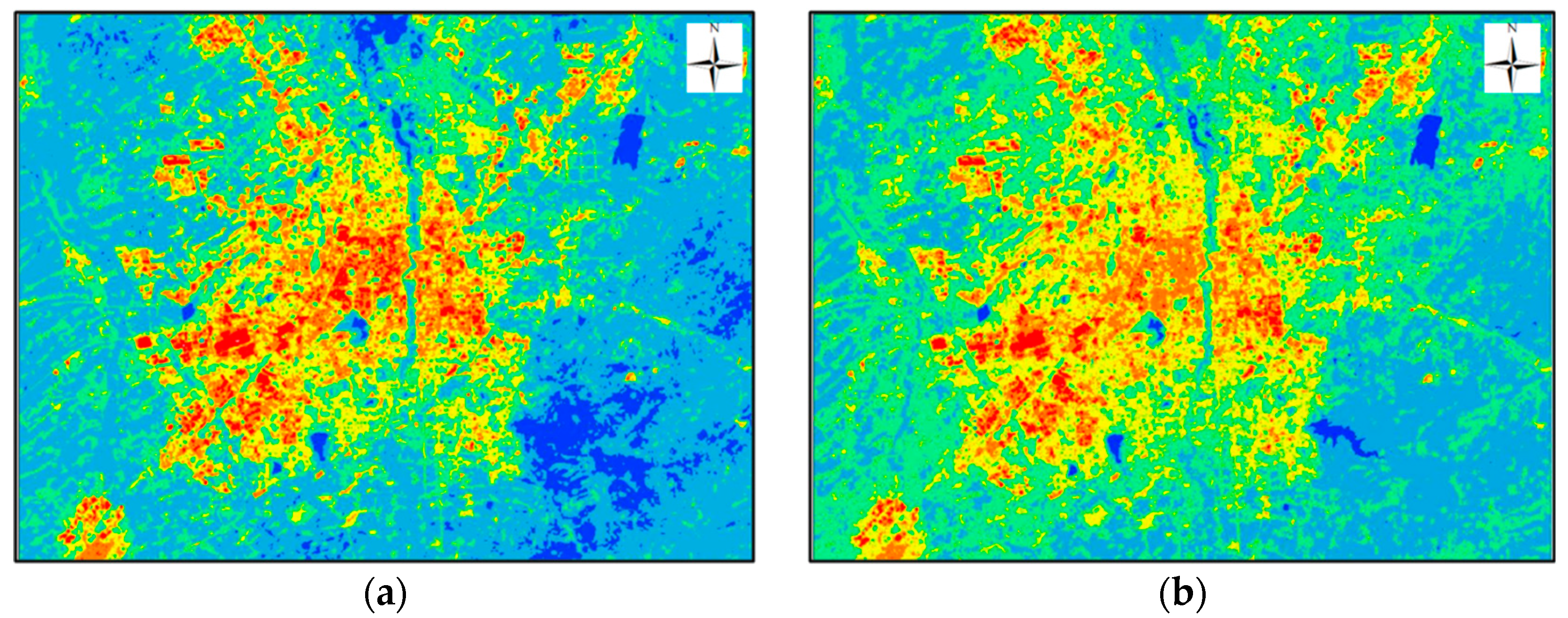
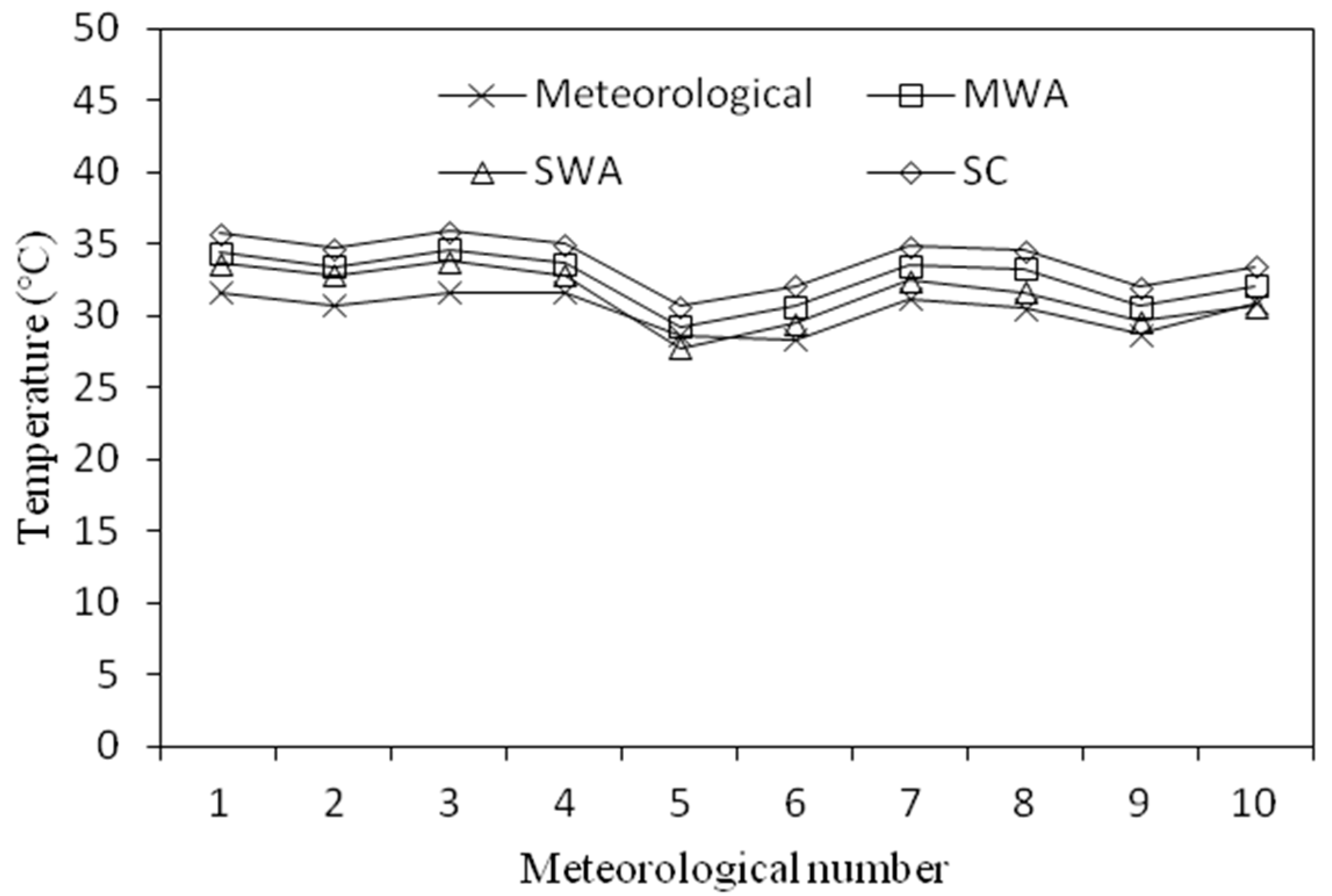
3.1. LST Retrieved by Three Methods
3.2. Verification of the Retrieved LST
4. Discussion
Author Contributions
Funding
Acknowledgments
Conflicts of Interest
References
- Friedel, M.J. Data-driven modeling of surface temperature anomaly and solar activity trends. Environ. Model. Softw. 2012, 37, 217–232. [Google Scholar] [CrossRef]
- Son, N.T.; Chen, C.F.; Chen, C.R.; Chang, L.Y.; Minh, V.Q. Monitoring agricultural drought in the Lower Mekong Basin using MODIS NDVI and land surface temperature data. Int. J. Appl. Earth Obs. Geoinf. 2012, 18, 417–427. [Google Scholar] [CrossRef]
- Maimaitiyiming, M.; Ghulam, A.; Tiyip, T.; Pla, F.; Latorre-Carmona, P.; Halik, Ü.; Sawut, M.; Caetano, M. Effects of green space spatial pattern on land surface temperature: Implications for sustainable urban planning and climate change adaptation. ISPRS J. Photogramm. Remote Sens. 2014, 89, 59–66. [Google Scholar] [CrossRef]
- Roy, D.P.; Wulder, M.A.; Loveland, T.R.; Woodcock, C.E.; Allen, R.G.; Anderson, M.C.; Helder, D.; Irons, J.R.; Johnson, D.M.; Kennedy, R.; et al. Landsat-8: Science and product vision for terrestrial global change research. Remote Sens. Environ. 2014, 145, 154–172. [Google Scholar] [CrossRef]
- Montanaro, M.; Gerace, A.; Lunsford, A.; Reuter, D. Stray Light Artifacts in Imagery from the Landsat 8 Thermal Infrared Sensor. Remote Sens. 2014, 6, 10435–10456. [Google Scholar] [CrossRef]
- Gerace, A.; Montanaro, M. Derivation and validation of the stray light correction algorithm for the thermal infrared sensor onboard Landsat 8. Remote Sens. Environ. 2017, 191, 246–257. [Google Scholar] [CrossRef]
- United States Geological Survey. Landsat 8 Operational Land Imager and Thermal Infrared Sensor Calibration Notices. Available online: http://landsat.usgs.gov/calibration_notices.php (accessed on 13 January 2014).
- García-Santos, V.; Cuxart, J.; Martínez-Villagrasa, D.; Jiménez, A.M.; Simó, G. Comparison of Three Methods for Estimating Land Surface Temperature from Landsat 8-TIRS Sensor Data. Remote Sens. 2018, 10, 1450. [Google Scholar] [CrossRef]
- Meng, X.; Cheng, J.; Zhao, S.; Liu, S.; Cheng, J. Estimating Land Surface Temperature from Landsat-8 Data using the NOAA JPSS Enterprise Algorithm. Remote Sens. 2019, 11, 155. [Google Scholar] [CrossRef]
- Qin, Z.; Karnieli, A.; Berliner, P. A mono-window algorithm for retrieving land surface temperature from Landsat TM data and its application to the Israel-Egypt border region. Int. J. Remote Sens. 2001, 22, 3719–3746. [Google Scholar] [CrossRef]
- McMillin, L.M. Estimation of sea surface temperaturesfrom two infrared window measurements with different absorption. J. Geophys. Res. 1975, 80, 80–82. [Google Scholar] [CrossRef]
- Jiménez-Muñoz, J.C.; Sobrino, J.A. A generalized single-channel method for retrieving land surface temperature from remote sensing data. J. Geophys. Res. Atmos. 2003, 108. [Google Scholar] [CrossRef]
- Wang, F.; Qin, Z.; Song, C.; Tu, L.; Karnieli, A.; Zhao, S. An Improved Mono-Window Algorithm for Land Surface Temperature Retrieval from Landsat 8 Thermal Infrared Sensor Data. Remote Sens. 2015, 7, 4268–4289. [Google Scholar] [CrossRef]
- Rozenstein, O.; Qin, Z.; Derimian, Y.; Karnieli, A. Derivation of land surface temperature for Landsat-8 TIRS using a split window algorithm. Sensors 2014, 14, 5768–5780. [Google Scholar] [CrossRef]
- Jiménez-Muñoz, J.C.; Sobrino, J.A.; Skokovic, D.; Mattar, C.; Cristóbal, J. Land Surface Temperature Retrieval Methods From Landsat-8 Thermal Infrared Sensor Data. IEEE Geosci. Remote Sens. Lett. 2014, 11, 1840–1843. [Google Scholar] [CrossRef]
- Yang, C.; He, X.; Wang, R.; Yan, F.; Yu, L.; Bu, K.; Yang, J.; Chang, L.; Zhang, S. The Effect of Urban Green Spaces on the Urban Thermal Environment and Its Seasonal Variations. Forests 2017, 8, 153. [Google Scholar] [CrossRef]
- Jin, M.; Li, J.; Wang, C.; Shang, R. A Practical Split-Window Algorithm for Retrieving Land Surface Temperature from Landsat-8 Data and a Case Study of an Urban Area in China. Remote Sens. 2015, 7, 4371–4390. [Google Scholar] [CrossRef]
- Ahn, Y.H.; Shanmugam, P.; Lee, J.H.; Kang, Y.Q. Application of satellite infrared data for mapping of thermal plume contamination in coastal ecosystem of Korea. Mar. Environ. Res. 2006, 61, 186–201. [Google Scholar] [CrossRef]
- Chatterjee, R.S.; Singh, N.; Thapa, S.; Sharma, D.; Kumar, D. Retrieval of land surface temperature (LST) from landsat TM6 and TIRS data by single channel radiative transfer algorithm using satellite and ground-based inputs. Int. J. Appl. Earth Obs. Geoinf. 2017, 58, 264–277. [Google Scholar] [CrossRef]
- Coll, C.; Caselles, V.; Valor, E.; Niclòs, R. Comparison between different sources of atmospheric profiles for land surface temperature retrieval from single channel thermal infrared data. Remote Sens. Environ. 2012, 117, 199–210. [Google Scholar] [CrossRef]
- Sobrino, J.A.; Jimenez-Munoz, J.C.; Soria, G.; Romaguera, M.; Guanter, L.; Moreno, J.; Plaza, A.; Martinez, P. Land Surface Emissivity Retrieval From Different VNIR and TIR Sensors. IEEE Trans. Geosci. Remote Sens. 2008, 46, 316–327. [Google Scholar] [CrossRef]
- Yang, C.; He, X.; Yan, F.; Yu, L.; Bu, K.; Yang, J.; Chang, L.; Zhang, S. Mapping the Influence of Land Use/Land Cover Changes on the Urban Heat Island Effect—A Case Study of Changchun, China. Sustainability 2017, 9, 312. [Google Scholar] [CrossRef]
- Coll, C.; Caselles, V.; Galve, J.M.; Valor, E.; Niclòs, R.; Sánchez, J.M.; Rivas, R. Ground measurements for the validation of land surface temperatures derived from AATSR and MODIS data. Remote Sens. Environ. 2005, 97, 288–300. [Google Scholar] [CrossRef]
- Pinker, R.T.; Sun, D.; Hung, M.-P.; Li, C.; Basara, J.B. Evaluation of Satellite Estimates of Land Surface Temperature from GOES over the United States. J. Appl. Meteorol. Climatol. 2009, 48, 167–180. [Google Scholar] [CrossRef]
- Wan, Z.; Li, Z.L. Radiance-based validation of the V5 MODIS land-surface temperature product. Int. J. Remote Sens. 2008, 29, 5373–5395. [Google Scholar] [CrossRef]
- Coll, C.; Valor, E.; Galve, J.M.; Mira, M.; Bisquert, M.; García-Santos, V.; Caselles, E.; Caselles, V. Long-term accuracy assessment of land surface temperatures derived from the Advanced Along-Track Scanning Radiometer. Remote Sens. Environ. 2012, 116, 211–225. [Google Scholar] [CrossRef]
- Qian, Y.-G.; Li, Z.-L.; Nerry, F. Evaluation of land surface temperature and emissivities retrieved from MSG/SEVIRI data with MODIS land surface temperature and emissivity products. Int. J. Remote Sens. 2013, 34, 3140–3152. [Google Scholar] [CrossRef]
- Trigo, I.F.; Monteiro, I.T.; Olesen, F.; Kabsch, E. An assessment of remotely sensed land surface temperature. J. Geophys. Res. Atmos. 2008, 113, 1–12. [Google Scholar] [CrossRef]
- Yang, L.; Cao, Y.; Zhu, X.; Zeng, S.; Yang, G.; He, J.; Yang, X. Land surface temperature retrieval for arid regions based on Landsat-8 TIRS data: A case study in Shihezi, Northwest China. J. Arid Land 2014, 6, 704–716. [Google Scholar] [CrossRef]
- Ren, Z.; Zheng, H.; HE, X.; Zhang, D.; Yu, X. Estimation of the Relationship Between Urban Vegetation Configuration and Land Surface Temperature with Remote Sensing. J. Indian Soc. Remote Sens. 2014, 43, 89–100. [Google Scholar] [CrossRef]
- Gillespie, A.; Rokugawa, S.; Matsunaga, T.; Cothern, J.S.; Hook, S.; Kahle, A.B. A temperature and emissivity separation algorithm for Advanced Spaceborne Thermal Emission and Reflection Radiometer (ASTER) images. IEEE Trans. Geosci. Remote Sens. 1998, 36, 1113–1126. [Google Scholar] [CrossRef]
- Momeni, M.; Saradjian, M. Evaluating NDVI-based emissivities of MODIS bands 31 and 32 using emissivities derived by day/night LST algorithm. Remote Sens. Environ. 2007, 106, 190–198. [Google Scholar] [CrossRef]
- Barsi, J.A.; Barker, J.L.; Schott, J.R. An Atmospheric Correction Parameter Calculator for a Single Thermal Band Earth-Sensing Instrument. In Proceedings of the IEEE International Geoscience and Remote Sensing Symposium, Toulouse, France, 21–25 July 2003; Volume 3, p. 37477. [Google Scholar]
- Yu, X.; Guo, X.; Wu, Z. Land Surface Temperature Retrieval from Landsat 8 TIRS—Comparison between Radiative Transfer Equation-Based Method, Split Window Algorithm and Single Channel Method. Remote Sens. 2014, 6, 9829–9852. [Google Scholar] [CrossRef] [Green Version]
- Price, J.C. Land surface temperature measurements from the split window channels of the NOAA 7 Advanced Very High Resolution Radiometer. J. Geophys. Res. Atmos. 1984, 89, 231–237. [Google Scholar] [CrossRef]
- Becker, F.; Li, Z.-L. Towards a local split window method over land surfaces. Int. J. Remote Sens. 1990, 11, 369–393. [Google Scholar] [CrossRef]
- Jiménez-Muñoz, J.C.; Cristóbal, J.; Sobrino, J.A.; Sòria, G.; Ninyerola, M.; Pons, X. Revision of the Single-Channel Algorithm for Land Surface Temperature Retrieval From Landsat Thermal-Infrared Data. IEEE Trans. Geosci. Remote Sens. 2009, 47, 339–349. [Google Scholar] [CrossRef]
- Jiménez-Muñoz, J.C.; Sobrino, J.A. A Single-Channel Algorithm for Land-Surface Temperature Retrieval From ASTER Data. IEEE Geosci. Remote Sens. Lett. 2010, 7, 176–179. [Google Scholar] [CrossRef]
- Liston, G.E.; Elder, K. A Meteorological Distribution System for High-Resolution Terrestrial Modeling (MicroMet). J. Hydrometeorol. 2006, 7, 217–234. [Google Scholar] [CrossRef] [Green Version]
- Zeng, L.; Wardlow, B.; Tadesse, T.; Shan, J.; Hayes, M.; Li, D.; Xiang, D. Estimation of Daily Air Temperature Based on MODIS Land Surface Temperature Products over the Corn Belt in the US. Remote Sens. 2015, 7, 951–970. [Google Scholar] [CrossRef] [Green Version]
- Prihodko, L.; Goward, S.N. Estimation of air temperature from remotely sensed surface observations. Remote Sens. Environ. 1997, 60, 335–346. [Google Scholar] [CrossRef]
- Nemani, R.R.; Running, S.W. Estimation of Regional Surface Resistance to Evapotranspiration from NDVI and Thermal-IR AVHRR Data. J. Appl. Meteorol. 1989, 28, 276–284. [Google Scholar] [CrossRef]
- Yuan, F.; Bauer, M.E. Comparison of impervious surface area and normalized difference vegetation index as indicators of surface urban heat island effects in Landsat imagery. Remote Sens. Environ. 2007, 106, 375–386. [Google Scholar] [CrossRef]


| M | A | |||
|---|---|---|---|---|
| Band 10 | 0.0003342 | 0.1 | 774.89 | 1321.08 |
| Band 11 | 0.0003342 | 0.1 | 480.89 | 1201.14 |
| Temperature Range | a10 | b10 | |
|---|---|---|---|
| 20–70 °C | −70.1775 | 0.4581 | 0.9997 |
| 0–50 °C | −62.7182 | 0.4339 | 0.9996 |
| −20–30 °C | −55.4276 | 0.4086 | 0.9996 |
| Band 10 | 0.991 | 0.984 | 0.964 | 0.959 | 0.958 |
| Band 11 | 0.986 | 0.980 | 0.970 | 0.962 | 0.969 |
| Atmospheres | Linear Relations Equations |
|---|---|
| Tropical model | Ta = 17.9769 + 0.9172 |
| Mid-latitude summer | Ta = 16.0110 + 0.9262 |
| Mid-latitude winter | Ta = 19.2704 + 0.9112 |
| Profile | Estimation Equation | R2 | SEE (Standard Error of Estimate) |
|---|---|---|---|
| 1976 US Standard | = −0.1146ω + 1.0286 | 0.9882 | 0.0094 |
| = −0.1568ω + 1.0083 | 0.9947 | 0.0086 | |
| Mid-latitude summer | = −0.1134ω + 1.0335 | 0.986 | 0.0101 |
| = −0.1546ω + 1.0078 | 0.996 | 0.0073 |
| T Range (°C) | ||||||||
|---|---|---|---|---|---|---|---|---|
| 0–30 | −59.1391 | 0.4213 | 0.9991 | 0.0424 | −63.3921 | 0.4565 | 0.9991 | 0.0438 |
| 0–40 | −60.9196 | 0.4276 | 0.9985 | 0.0746 | −65.2240 | 0.4629 | 0.9985 | 0.0769 |
| 10–40 | −62.8065 | 0.4338 | 0.9992 | 0.0415 | −67.1728 | 0.4694 | 0.9992 | 0.0427 |
| 10–50 | −64.6081 | 0.4399 | 0.9986 | 0.0730 | −69.0215 | 0.4756 | 0.9986 | 0.0750 |
| Emissivity | Transmission | Average Ratio | |||
|---|---|---|---|---|---|
| 0.96 | 0.7 | 0.672 | 0.3084 | 0.458929 | 0.447351 |
| 0.97 | 0.7 | 0.679 | 0.3063 | 0.451105 | |
| 0.98 | 0.7 | 0.686 | 0.3042 | 0.44344 | |
| 0.99 | 0.7 | 0.693 | 0.3021 | 0.435931 | |
| 0.96 | 0.8 | 0.768 | 0.2064 | 0.26875 | 0.261599 |
| 0.97 | 0.8 | 0.776 | 0.2048 | 0.263918 | |
| 0.98 | 0.8 | 0.784 | 0.2032 | 0.259184 | |
| 0.99 | 0.8 | 0.792 | 0.2016 | 0.254545 | |
| 0.96 | 0.9 | 0.864 | 0.1036 | 0.119907 | 0.116553 |
| 0.97 | 0.9 | 0.873 | 0.1027 | 0.11764 | |
| 0.98 | 0.9 | 0.882 | 0.1018 | 0.11542 | |
| 0.99 | 0.9 | 0.891 | 0.1009 | 0.113244 |
| Number | Local Meteorological | Mono-Window Algorithm | Split Window Algorithm | Single Channel Method | |||
|---|---|---|---|---|---|---|---|
| Temperature (°C) | Temperature (°C) | Δ | Temperature (°C) | Δ | Temperature (°C) | Δ | |
| 1 | 31.60 | 34.38 | 2.78 | 33.63 | 2.03 | 35.72 | 4.12 |
| 2 | 30.70 | 33.40 | 2.70 | 32.79 | 2.09 | 34.71 | 4.01 |
| 3 | 31.60 | 34.59 | 2.99 | 33.78 | 2.18 | 35.90 | 4.30 |
| 4 | 31.65 | 33.63 | 1.98 | 32.83 | 1.18 | 34.97 | 3.32 |
| 5 | 28.65 | 29.26 | 0.61 | 27.76 | −0.89 | 30.63 | 1.98 |
| 6 | 28.35 | 30.69 | 2.34 | 29.47 | 1.12 | 32.04 | 3.69 |
| 7 | 31.15 | 33.46 | 2.31 | 32.45 | 1.30 | 34.82 | 3.67 |
| 8 | 30.50 | 33.26 | 2.76 | 31.66 | 1.16 | 34.56 | 4.06 |
| 9 | 28.70 | 30.62 | 1.92 | 29.58 | 0.88 | 32.00 | 3.30 |
| 10 | 30.9 | 32.09 | 1.19 | 30.66 | −0.24 | 33.43 | 2.53 |
| Average difference | 2.16 | 1.08 | 3.5 | ||||
| RMSE | 0.72 | 0.94 | 0.71 | ||||
© 2019 by the authors. Licensee MDPI, Basel, Switzerland. This article is an open access article distributed under the terms and conditions of the Creative Commons Attribution (CC BY) license (http://creativecommons.org/licenses/by/4.0/).
Share and Cite
Wang, L.; Lu, Y.; Yao, Y. Comparison of Three Algorithms for the Retrieval of Land Surface Temperature from Landsat 8 Images. Sensors 2019, 19, 5049. https://doi.org/10.3390/s19225049
Wang L, Lu Y, Yao Y. Comparison of Three Algorithms for the Retrieval of Land Surface Temperature from Landsat 8 Images. Sensors. 2019; 19(22):5049. https://doi.org/10.3390/s19225049
Chicago/Turabian StyleWang, Lei, Yao Lu, and Yunlong Yao. 2019. "Comparison of Three Algorithms for the Retrieval of Land Surface Temperature from Landsat 8 Images" Sensors 19, no. 22: 5049. https://doi.org/10.3390/s19225049