Next Article in Journal
A Simply Equipped Fourier Ptychography Platform Based on an Industrial Camera and Telecentric Objective
Previous Article in Journal
Combination of an Axicon Fiber Tip and a Camera Device into a Sensitive Refractive Index Sensor
 
 
Correction published on 4 November 2020, see Sensors 2020, 20(21), 6274.
Article

Comparative Analysis between Error-State and Full-State Error Estimation for KF-Based IMU/GNSS Integration against IMU Faults

School of Electronic and Information Engineering, Beihang University, Beijing 100191, China
*
Author to whom correspondence should be addressed.
Sensors 2019, 19(22), 4912; https://doi.org/10.3390/s19224912
Submission received: 9 October 2019 / Revised: 3 November 2019 / Accepted: 7 November 2019 / Published: 11 November 2019
(This article belongs to the Section Remote Sensors)

Abstract

:
Considering the inertial measurement unit (IMU) faults risk of an unmanned aerial vehicle (UAV), this paper provides an analysis of the error overboundings of position estimation in a tightly coupled IMU/global navigation satellite system (GNSS) integrated architecture under the IMU fault conditions using an error-state EKF-based approach and provides a comparison to a recently published EKF-based full state method. Simulation results show that both the error overboundings of the error-state and full-state EKFs can fit the state error against the IMU faults, but the error-state EKF is more suitable for UAV navigation system integrity assurance due to its higher calculation efficiency. This study will be extended to the integrity monitoring of multisensor systems.

1. Introduction

Unmanned aerial vehicles (UAVs) are widely used in many aspects of our daily life. The application of UAVs will permeate more aspects of public life in the near future. To ensure the safety of a UAV, its navigation solution should be fully protected by an integrity assurance mechanism, including real-time fault detection and an integrity risk evaluation. Integrity risk is the probability of hazardous misleading information (HMI) [1] and can be evaluated by the error overboundings (i.e., protection levels (PLs)) of the estimated position solution corresponding to the required probability of HMI, i.e., the integrity risk requirement [2,3].
An UAV usually adopts an inertial measurement unit (IMU)/global navigation satellite system (GNSS) integrated navigation system. The configuration of the IMU on UAVs can be performed according to the practical application requirements. UAVs similar to the DJI Phantom series use two IMUs to provide redundant measurements [4]. The experimental test carried out by Rhudy uses four IMUs to provide redundant IMU data [5]. Although the redundantly configured IMU can be used to detect IMU faults, there is still a probability of missed detection, and the fault risk of IMU still exists. Moreover, the low-cost micro-electromechanical system (MEMS) IMU on an UAV has a lower reliability and is more vulnerable to the flight environment than the fiber-optic strapdown IMU on civil aviation aircraft. Giorgio showed that IMUs are more prone to malfunction in high-vibration environments, where UAVs typically operate [6]. Bhatti listed the fault types of IMU sensors and summarized the potential causes of each fault type [7]. The IMU also has a high fault risk in the integrated navigation system for UAVs [8]. Therefore, IMU faults cannot be ignored in the integrity assurance mechanism of UAVs’ integrated navigation architecture.
Many studies have been carried out to assure the navigation integrity of UAVs. However, most studies still place emphasis on assuring the integrity of the GNSS. Some of the studies focus on researching GNSS integrity augmentation systems, which apply GNSS monitoring technology in civil aviation to UAVs. For instance, Pullen developed a local-area differential GNSS architecture around the concept of local-area UAV network operations, which can assure the integrity of UAVs against GNSS faults with a low cost [9]. Lee proposed a high-integrity navigation architecture for the integrated IMU/LAD-GNSS system with a filter based on the extended Kalman filter (EKF), which can support continuous and reliable navigation by overcoming the GNSS’ signal vulnerability [10]. Kim presented a LAD-GNSS architecture for UAVs that communicates with ground subsystems in real time, reducing the vertical PLs by approximately 16% [11].
Other studies have utilized the EKF innovation or residual to monitor the GNSS integrity, which is known as IMU-aided GNSS integrity monitoring. There are two aspects of this research—IMU-aided GNSS fault detection and integrity risk evaluation against a GNSS fault. For the first aspect, Brenner proposed the multiple solution separation (MSS) method [12], Diesel investigated the autonomous integrity monitoring by extrapolation (AIME) method [13], and Crespillo performed a comparison between innovation-based and residual-based fault detection in the EKF for GNSS/INS hybridization [14]. They are all effective for GNSS fault detection in an IMU/GNSS navigation system. For the second aspect, Joerger evaluated the integrity risk in a sequential Kalman filter (KF) by quantifying the worst-case integrity risk based on the relationship between the state error and the GNSS range residual to construct monitor test statistics using a least square (LS) expression [15]. Tanil instead used the recursive expression and applied it to GNSS spoofing detection [16]. Bhattacharyya proposed the real-time PLs computation through the residual-based RAIM algorithm [17]. All of these approaches can monitor the integrity of the GNSS in the IMU/GNSS integrated navigation system.
Different from the above studies, Lee proposed an integrity assurance mechanism for an EKF-based IMU/GNSS integrated system against IMU faults [18]. She calculated the PLs using the EKF innovations and additional uncertain noise boundary terms, by deriving the IMU faults propagation process in the EKF [18]. In her study, the full-state inertial navigation equations, including the attitude, velocity, and position update equations, were used as the EKF system propagation equations. Moreover, the velocity update equation was used as an example to explain how the IMU faults propagate in the EKF.
In our study, different from the method published by Lee et al. [18], the error-state inertial navigation equations, including the attitude error, the velocity error, and the position error update equations, were used to analyze the IMU faults propagation process which are more commonly used as the EKF system propagation equations in IMU/GNSS integrated navigation than the full-state inertial navigation equations [18,19,20]. While being inspired by the previous published research in this area [16,17,18,19,20], the error overboundings against the IMU faults for the EKF state estimation using the error-state inertial navigation equation is derived in this paper. Moreover, the error overboundings using error-state and full-state inertial navigation equations are compared to determine which kind is more conducive to assuring the integrity for the IMU/GNSS integrated navigation architecture against IMU faults. After using the inertial navigation error equation, the magnitude of each dimension of the state vector keep close or consistent, and the occurrence of singular matrices in the filtering calculation process is avoided, which will shorten the filtering time, improve the converge speed, and increase the calculation efficiency. To simplify the description below, the EKF using the full-state inertial navigation equations is named the full-state EKF, whereas the EKF using the error-state inertial navigation equation is named the error-state EKF.
Accordingly, the remainder of this paper is organized as follows: (1) the general structures of the IMU/GNSS integrated navigation architecture using the IMU error-state model are introduced, (2) the detailed IMU faults propagation process in the error-state EKF is specially derived, (3) a description of the real-time error overboundings (PLs) equations in the error-state EKF for IMU faults based on innovations, (4) the simulations for the error overboundings calculation under IMU faults are presented, and (5) the summary and concluding remarks close the paper.

2. Architecture of the IMU/GNSS Integrated Navigation System

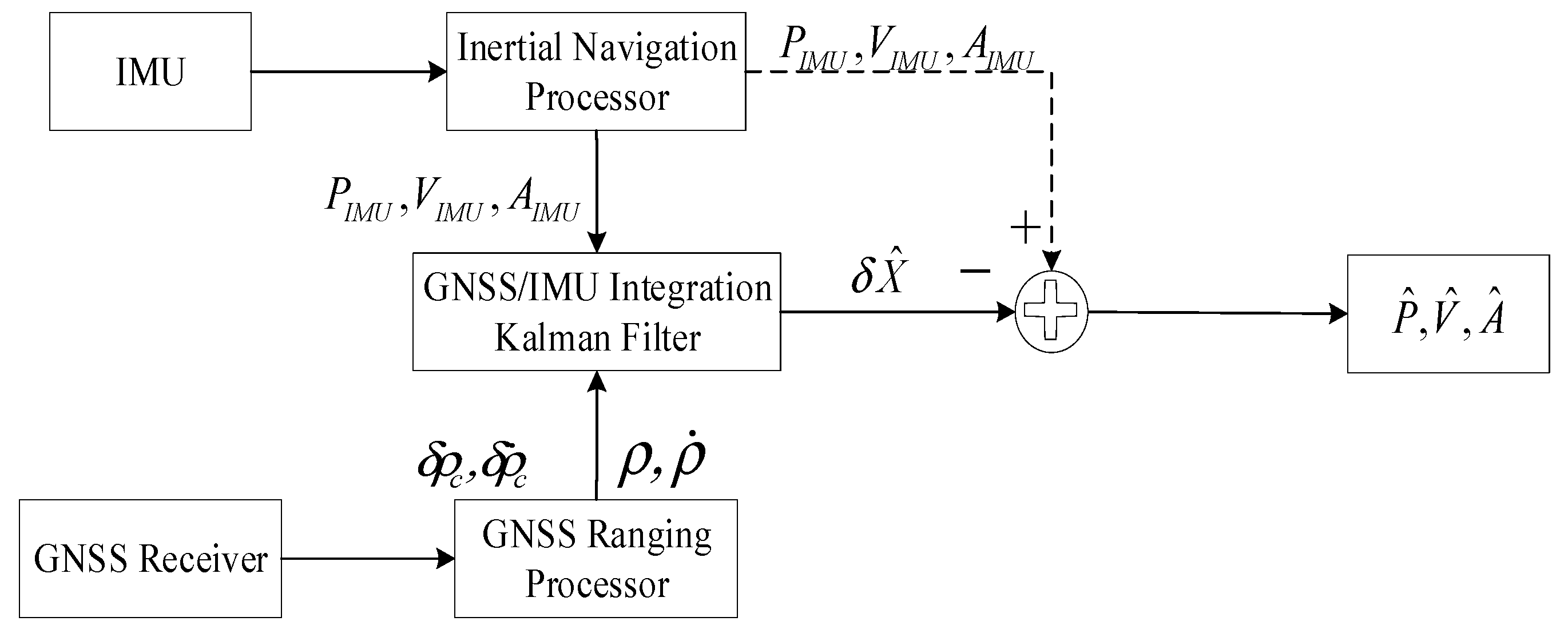
2.1. IMU/GNSS Integration Architecture

Figure 1 illustrates an overview of the EKF-based tightly coupled IMU/GNSS integration architecture. The inputs are the GNSS pseudo-range, ρ , pseudo-range rate, ρ ˙ , GNSS receiver clock offset, δ ρ c , and GNSS receiver drift, δ ρ ˙ c , from the GNSS ranging processor and the IMU position, P I M U , velocity, V I M U , and attitude, A I M U , navigation parameters from the inertial navigation processor. The outputs of the integrated navigation system are the corrected IMU position, P ^ , velocity, V ^ , and attitude, A ^ . The integration is completed in the range domain. In this study, the error-state inertial navigation equations based EKF (i.e., the error-state EKF) was used for the IMU/GNSS integration architecture, and the outputs of the IMU/GNSS integration Kalman filter were the UAV navigation parameter error estimation, δ X ^ [21].

2.2. Error-State EKF Model

Using the error-state IMU equations as the system propagation equation, the state vector includes the IMU attitude error, IMU velocity error, IMU position error, inertial sensor biases, and GNSS receiver clock offset and drift for the error-state EKF [22]. The EKF is described as a system propagation equation (Equation (1)) and a measurement update equation (Equation (2)) [6]. In the measurement updates step, the GNSS pseudo-range and pseudo-range rate measurements are used for the measurement update, and the difference between the GNSS pseudo-range, GNSS pseudo-range rate and the corresponding predicted IMU pseudo-range, IMU pseudo-range rate constitute the EKF innovation. There is another expression of the system propagation equation, the full-state inertial navigation equations based EKF (i.e., the full-state EKF). For either the full-state or error-state in EKF, the essence is to estimate the state error. However, there is a difference between the error-state EKF and the full-state EKF in the system propagation step, the control input is added to the full-state EKF (Appendix A):
X ^ k = Φ k X ^ k 1 + Γ w k w k
X ^ k = X ^ k + K k ( Z k H k X ^ k ) r k
where X ^ k is the predicted error-state vector at epoch k, X ^ k is the measurement updated error-state vector at epoch k, Φk is the dynamic state transition matrix at epoch k, Γwk is the process noise matrix at epoch k, w k is the process noise vector at epoch k, K k is the Kalman gain at epoch k (Appendix B.1), Z k is the estimate of the measurement produced by the states estimated by the Kalman filter, H k is the measurement matrix at epoch k (Appendix B.1), and r k is the EKF innovation vector at epoch k.

3. Error Overboundings against IMU Faults

Different from the full-state EKF, the error-state EKF has no input of the control quantity during the entire filtering process. Compared with the full-state EKF, the error-state EKF keeps the magnitude of each dimension of the state vector close or consistent, which avoids the occurrence of singular matrices in the filtering calculation process, reduces the convergence time and improves the calculation efficiency.
This part analyzes the propagation process of IMU faults for the error-state EKF in detail. Through the analysis, the recursive propagation equation between adjacent epochs of the EKF state error is obtained. Based on the EKF state error propagation equation and the EKF innovation equation, the error overboundings of the EKF state error are given.

3.1. IMU Faults Propagation in the Error-State EKF

In this section, the IMU faults propagation process in the state vector for the error-state EKF is explained. While following a similar approach, it is worth mentioning that the method derived here is a different approach from the work published by Lee et al. [18] where error states instead of full navigation states are considered. The differences between the output measurement value and the true value of the IMU are expressed in Equation (3):
{ δ φ β α = φ ˜ β α φ β α δ v β α r = v ˜ β α r v β α r δ r β α r = r ˜ β α r r β α r
where “~” represents the measurement value, φ β α is the attitude vector (rad), v β α r is the velocity vector (m/s), and r β α r is the position vector (m).
The inertial navigation error equations in the Earth-centered, Earth-fixed (ECEF) coordinate frame can be seen in Equation (4), including the attitude error, velocity error, and position error update equations:
δ φ ˙ e b e = C b e ( [ ω ˜ i b b × ] [ ω i b b × ] ) [ ω i e e × ] ( φ ˜ e b e φ e b e ) δ v ˙ e b e = C b e ( f ˜ i b b f i b b ) 2 [ ω i e e × ] ( v ˜ e b e v e b e ) + g ^ e g e δ r ˙ e b e = v ˜ e b e v e b e
where C b e is the coordinate transformation matrix from the body frame to the Earth frame (a detailed expression can be found in Appendix B.2), ω i e e is the Earth rotation rate (rad/s), g e is the gravity vector in the Earth-centered, Earth-fixed frame (m/s2), and [ × ] represents the calculation of a skew-symmetric matrix.
Neglecting the effects of gravity errors, Equation (4) can be simplified as
δ φ ˙ e b e = C b e δ [ ω i b b × ] [ ω i e e × ] δ φ e b e δ v ˙ e b e = C b e δ f i b b 2 [ ω i e e × ] δ v e b e δ r ˙ e b e = δ v e b e .
Figure 2 shows the updating process of the attitude, velocity, and position in the ECEF coordinate frame for the IMU. When IMU faults occur in the gyroscope or accelerometer, the computed attitude, velocity, and position are sequentially affected, finally resulting in position errors.
Under the condition of a faulty IMU, the inertial navigation error equation in Equation (5) becomes Equation (6), where the apostrophe (’) indicates the faulty parameter. The parameters affected by the fault are expressed as the sum of a normal error term and a faulty additional error term, as shown in Equation (7):
δ φ ˙ e b e = C b e ( δ [ ω i b b × ] ) [ ω i e e × ] δ φ e b e δ v ˙ e b e = ( C b e ) ( δ f i b b ) 2 [ ω i e e × ] δ v e b e δ r ˙ e b e = ( δ v e b e )
δ ω i b b = δ ω i b b + Δ ω i b b δ f i b b = δ f i b b + Δ f i b b δ v e b e = δ v e b e + Δ v e b e .
Substituting Equation (7) into Equation (6), the inertial navigation error equation under the IMU faults condition can be shown as
δ φ ˙ e b e = C b e ( δ [ ω i b b × ] + Δ ω i b b ) [ ω i e e × ] δ φ e b e δ v ˙ e b e = ( C b e + Δ C b e ) ( δ f i b b + Δ f i b b ) 2 [ ω i e e × ] δ v e b e δ r ˙ e b e = δ v e b e + Δ v e b e .
Rearrange Equation (8),
δ φ ˙ e b e = C b e δ [ ω i b b × ] [ ω i e e × ] δ φ e b e + C b e Δ ω i b b f δ φ ˙ e b e δ v ˙ e b e = C b e δ f i b b 2 [ ω i e e × ] δ v e b e + C b e Δ f i b b + Δ C b e ( δ f i b b + Δ f i b b ) f δ v ˙ e b e δ r ˙ e b e = δ v e b e + Δ v e b e f δ r ˙ e b e
where f δ φ ˙ b e , f δ v ˙ e b e , and f δ r ˙ e b e represent the resultant bias vectors for the attitude, velocity, and position error states due to the IMU faults. In the EKF, the accelerometer measurement of the specific force f i b , m e a s b is represented as Equation (10), which includes the true specific force, the accelerometer bias, and the process noise. In addition, the gyroscope measurement of the angular rate, ω i b , m e a s b , is represented as Equation (11), which includes the true angular rate, the gyroscope bias, a g-dependent bias related to the specific force, and process noise. The accelerometer bias and gyroscope bias are usually modeled as constant errors [23]:
f i b , m e a s b = f i b b + b a + w a
ω i b , m e a s b = ω i b b + b g + G g f i b b + w g .
According to Equations (10) and (11), the accelerometer measurement of the specific force error and the gyroscope measurement of the angular rate error are derived from the accelerometer measurement of the specific force, f i b , m e a s b , and the gyroscope measurement of the angular rate, ω i b , m e a s b , as shown in Equation (12):
δ ω i b b = ω i b , m e a s b ω i b b = b g + G g f i b b + w g δ f i b b = f i b , m e a s b f i b b = b a + w a .
Substituting Equation (12) into Equation (9), the inertial navigation error equation under the IMU faults condition is
δ φ ˙ e b e = C b e [ ( b g + G g f i b b + w g ) × ] [ ω i e e × ] δ φ e b e + f δ φ ˙ e b e δ v ˙ e b e = C b e [ ( b a + w a ) × ] 2 [ ω i e e × ] δ v e b e + f δ v ˙ e b e δ r ˙ e b e = δ v e b e + f δ r ˙ e b e .
Rearranging Equation (13), the inertial navigation error equation under the IMU faults condition (Equation (8)) becomes a continuous form of an EKF error-state equation as a function of EKF error states, process noise, and the state fault vector, as shown in Equation (14):
δ φ ˙ e b e = [ ω i e e × ] δ φ e b e + C b e [ b g × ] F δ φ e b e δ φ e b e + C b e [ ( G g f i b b + w g ) × ] G g w g + f δ φ ˙ e b e δ v ˙ e b e = 2 [ ω i e e × ] δ v e b e + C b e [ b a × ] F δ v e b e δ v e b e + C b e [ w a × ] G a w a + f δ v ˙ e b e δ r ˙ e b e = δ v e b e + f δ r ˙ e b e .
Based on the integral relationship between the velocity and the position in the error-state inertial navigation equations, Equation (14) can be rewritten as
δ φ ˙ e b e = F δ φ e b e δ φ e b e + G g w g + f δ φ ˙ e b e δ v ˙ e b e = F δ v e b e δ v e b e + G a w a + f δ v ˙ e b e δ r ˙ e b e = F δ r e b e δ r e b e + G r w r + f δ r ˙ e b e .
Hence, an EKF state equation under the IMU faults condition generalized as Equation (16) in a continuous form. The error-state vector contains the IMU position error, the IMU velocity error, the IMU attitude error, accelerometer biases, gyroscope biases, the GNSS receiver offset, and the GNSS receiver drift:
X = F X + G w w + f X ˙
where
X = [ δ φ e b e δ v e b e δ r e b b b a b g δ ρ c δ ρ ˙ c ] , w = [ w a w g ] , f X ˙ = [ f δ φ ˙ e b e f δ v ˙ e b e f δ r ˙ e b e 0 3 0 3 0 0 ] , G w = [ 0 3 C b e C b e 0 3 0 3 0 3 0 3 0 3 0 3 0 3 0 0 0 0 ]
F = [ [ ω i e e × ] 0 3 0 3 0 3 C b e 0 0 [ ( C ^ b e f ^ i b b ) × ] 2 [ ω i e e × ] 0 C b e 0 3 0 0 0 3 I 3 0 0 3 0 3 0 0 0 3 0 3 0 3 0 3 0 3 0 0 0 3 0 3 0 3 0 3 0 3 0 0 0 0 0 0 0 0 I 0 0 0 0 0 0 0 ] .
The discrete form of Equation (16) is shown in Equation (17) [18]:
X k = Φ k X k 1 + ω k + f X k .
The discrete form of F is shown as
Φ [ I 3 [ ω i e e × ] τ s 0 3 0 3 0 3 C b e τ s 0 0 [ ( C ^ b e f ^ i b b ) × ] τ s I 3 2 [ ω i e e × ] τ s [ ω i e e × ] 2 τ s C b e τ s 0 3 0 0 0 3 I 3 τ s [ ω i e e × ] 2 τ s 2 I 3 τ s + [ ω i e e × ] τ s 2 / 2 0 3 0 3 0 0 0 3 0 3 0 3 I 3 0 3 0 0 0 3 0 3 0 3 0 3 I 3 0 0 0 0 0 0 0 I 3 τ s 0 0 0 0 0 0 I 3 ]
where τ s is the time interval of the adjacent propagation.
Thus, the predicted state under the IMU faults condition at epoch k is
X ^ k = Φ k X ^ k 1 + f X k .
Substituting Equation (19) into Equation (2), the measurement update state under the IMU faults condition at epoch k is [18]:
X ^ k = X ^ k + K k ( Z k H k X ^ k ) = Φ k X ^ k 1 + f x k + K k ( Z k H k ( Φ k X ^ k 1 + f X k ) ) = ( I K k H k ) ( Φ k X ^ k 1 + f X k ) + K k Z k
where K k is the Kalman gain matrix computed by the faulty state transition matrix due to the IMU faults measurements and H k is the measurement matrix at epoch k (Appendix B.1).
To simplify Equation (20), a matrix L k is introduced as Equation (21) [18]:
L k = ( I K k H k ) .
Subsequently, Equation (20) can be simplified as
X ^ k = L k Φ k X ^ k 1 + L k f x k + K k Z k .
According to Equation (22), the additional term due to the IMU faults measurement at epoch k is L k f X k .

3.2. EKF State Error Caused by IMU Faults

The true state can be defined as shown in Equation (23):
X k = Φ k X k 1 + ω k .
According to the previous study [18], the state error propagation between two adjacent epochs can be derived as follows:
In step 1, multiply the matrix L k by the true state, X k :
L k X k = L k ( Φ k X k 1 + ω k ) = L k Φ k X k 1 + L k ω k .
In step 2, subtract L k X k from X ^ k in Equation (22):
X ^ k L k X k = L k Φ k X ^ k 1 + L k f x k + K k Z k L k X k .
In step 3, substitute Z k = H k X k + v k into Equation (25):
X ^ k L k X k = L k Φ k X ^ k 1 + L k f X k + K k ( H k X k + v k ) L k ( Φ k X k 1 + ω k ) = L k Φ k ( X ^ k 1 X k 1 ) δ X k 1 + L k f X k + K k v k L k ω k + K k H k X k .
Substitute Equation (21) into Equation (26):
X ^ k X k δ X k = L k Φ k ( X ^ k 1 X k 1 ) δ x k 1 + L k f X k + K k v k L k ω k δ X k = L k Φ k δ X k 1 + L k f X k + K k v k L k ω k .

3.3. Error Overboundings

For the error-state EKF, the innovation at epoch k can be expressed as follows:
γ k = Z k H k X ^ k = H k X k + v k H k X ^ k = H k ( Φ k X k 1 + ω k ) + v k H k ( Φ k X ^ k 1 + f X k ) = H k Φ k ( X k 1 X ^ k 1 ) δ X k 1 + H k ω k + v k H k f X k = H k Φ k δ X k 1 + H k ω k + v k H k f X k .
As Equations (27) and (28) show, the final EKF state error and EKF innovation using the error-state EKF were the same as that obtained by the full-state EKF in [18]. Based on the method proposed in [18] for the full-state EKF, the error overboundings against the IMU faults for the error-state EKF can be expressed as Equation (29), which was originally derived in [18] for the full-state EKF.
P L e r r o r o v e r b o u n d i n g s = V k , p γ k ± K m d , I M U { σ V k , p v k , v + σ K k , p v k , v } .
As we expected, the final error overboundings equation (Equation (29)) can be expressed in an identical manner to those derived based on the full-state EKF in the previous study [18].

4. Simulation and Analysis

4.1. Simulation Conditions

Simulations were conducted to show the error overboundings for UAVs under the IMU faults condition using both the full-state EKF (Appendix C) and the error-state EKF. In the simulations, the GNSS measurement noise and the IMU gyroscope and accelerometer measurement noise were modeled as Gaussian white noise, and the corresponding noise parameters were also used in the error overboundings.
The specific UAV trajectory can be seen in Figure 3, configured as an integration of two 45° turns and one vertical climb. The simulation time was 7 min.
The IMU sensors were set as consumer-grade inertial sensors with the noise parameters listed in Table 1 [24]. In the simulation, a 24-satellite GPS constellation was used, and the mask angle was 7.5°. The GNSS measurement noise was introduced into the pseudo-ranges as white Gaussian noise with a mean of zero and a variance of 30 m2. The data update frequency was 5 Hz for the GNSS receiver and 100 Hz for the IMU sensors. The integrated Kalman filter update was only performed when the GNSS signal was updated, otherwise only the IMU output was used. The output frequency was 100 Hz, which was the same as the IMU update frequency.
All simulations were performed using MATLAB R2018a on a Windows 10 PC with 12 GB of RAM and an Intel Core i7-6700 3.4 GHz processor.

4.2. Simulation Under Injected IMU Gyroscope and Accelerometer Faults

For the simulations of the error overboundings, the prior probabilities of an IMU gyroscope and accelerometer sensor faults were assumed to be 10−3, considering the IMU hardware performance used for a low-cost use and consumer-grade inertial device [25]. In the simulation, the ramp IMU gyroscope and accelerometer faults, with magnitudes of 1.5 m/s2 in the accelerometer and 0.03 rad/s in the gyroscope, was injected into the IMU accelerometer and gyroscope for three axes after 200 s. The faults injection lasted 10 s.
As an example, the vertical position errors are presented as the red dotted curve, which is the difference between the EKF estimated vertical position and the true vertical position, in Figure 4. In addition, the vertical error overboundings (VPLerror.overboundings) are presented in Figure 4, as blue solid curves for the error-state EKF and green solid curves for the full-state EKF. In order to intuitively present the vertical state error in Figure 4, the state error is represented in Figure 5, as a blue dotted curve for the error-state EKF and a red solid curve for the full-state EKF. In this simulation, the value of Kmd,IMU was chosen to be 3.29, which overbounds the noise of the state bias estimates with a missed detection probability of 10−3 (Appendix B.3). The simulation results show that the overboundings had the same trend as the position error and that the position error can be accurately overbounded during UAV operations under the missed detection probability requirement. Moreover, the error overboundings of the two EKFs were the same when no fault occurred. When faults were injected, the error overboundings for the error-state were higher than the full-state; the reason for this is that the error-state EKF is more sensitive to the faults than the full-state EKF. The east and north state errors and overboundings (i.e., east error overboundings (EPLerror.overboundings), north error overboundings (NPLerror.overboundings)) are also presented in Figure 6 and Figure 7, respectively, which further proves that the position error can be accurately overbounded and that the error overboundings of the two EKFs are the same in all directions.

4.3. Computational Efficiency Comparison

To compare the efficiency of the full-state and the error-state EKFs in the error overboundings calculation, the filtering time at each epoch is recorded in Figure 8. The filtering time of the error-state EKF was lower and more stable than that of the full-state EKF. The average filtering time for the error-state EKF was approximately 7.573 × 10⁻⁴ s, 16.163% less than that for the full-state error, approximately 9.033 × 10⁻³ s. A detailed comparison can be seen in Table 2.
Actually, the filtering time required for sparse matrix operations is usually proportional to the number of arithmetic operations in the number of nonzero elements. In the system state propagation period, the state transition matrix Φk of the full-state EKF has more nonzero elements than that of the error-state EKF. As shown in Figure 8, taking, for example, the simulation times at 312.5 s and 357.5 s, there are distinct peaks for the full-state EKF because of the sparse matrices in the system propagation equation. Moreover, the convergence process of the EKF was evaluated by 3.66 times variance. As shown in Figure 9, the state error of the error-state EKF converged faster than the full-state EKF, the oscillation before convergence was smaller, and the convergence process was smoother.
To sum up, error-state EKF-based method and full-state EKF-based method are consistent in final equation expression and overbounding results of the error overboundings. However, the qualitative analysis result shows that error-state EKF-based method has a higher calculation efficiency and faster convergence speed, and the quantitative comparison result in Table 2 shows error-state EKF-based method has shorter filtering time.

5. Conclusions

A real-time full-state EKF vertical protection level (VPL) method against IMU sensor faults to assure navigation integrity is proposed in [18]. Based on the method, the final error overbounding equation against the IMU faults for the error-state EKF estimation can be expressed in an identical manner. The IMU faults propagation process was analyzed in this paper for the error-state EKF of tightly coupled IMU/GNSS integrated architecture. Accordingly, the error overboundings against the IMU faults was obtained. The error overboundings for the full-state and the error-state EKFs presented the same form in theoretical derivation, consisting of terms relating to the EKF innovation, the estimated bias, and the remaining position error. The simulation result shows that the derived error overboundings can fit the position error, reflecting the position error change caused by the IMU faults. Moreover, the error overboundings of the error-state EKF were the same as that of the full-state EKF in mathematical simulation. As the error-state EKF is more practical and its error overboundings calculation time was lower, the error-state EKF is recommended to assure the integrity of the IMU/GNSS integrated architecture for an UAV. The proposed error overbounding method with real collected data will be carried out in future work.

Author Contributions

W.L. and D.S. conceived of and designed the research. W.L. and D.S. performed the theoretical derivation, experiments, and analyzed the results. W.L. and D.S. wrote the paper. Z.W. and K.F. were responsible for data acquisitions and data processing. Z.W. was responsible for project management. W.L., D.S., Z.W., and K.F. finalized the manuscript version to be published.

Funding

The work was carried out with financial support from the National Natural Science Foundation of China (Grant Nos. 61871012 and U1833125), the major project on the second satellite navigation system of China (Grant No. GFZX0305030106) and the Shaanxi Key Laboratory of Integrated and Intelligent Navigation (SKLIIN-20190205).

Acknowledgments

The authors would like to thank many people in the National Key Laboratory of CNS/ATM for their advice and interest.

Conflicts of Interest

The authors declare no conflict of interest.

Appendix A. Full-State EKF Model

Using the full-state IMU equations as the system propagation equation, the state vector includes the attitude, velocity, position, inertial sensor biases, and GNSS receiver clock offset and drift for the full-state EKF. The EKF is described as a system propagation equation (Equation (A1)) and a measurement update equation (Equation (A2)). In the system state propagation step, the IMU measurements of the specific force f i b , m e a s b and angular rate ω i b , m e a s b are considered as the control input (All the nomenclatures can be seen in Appendix D). In the measurement update step, the GNSS pseudo-range and pseudo-range rate measurements are used for the measurement update:
X ^ k = Φ k X ^ k 1 + Γ u k u k + Γ w k w k
X ^ k = X ^ k + K k ( Z k H k X ^ k )
where X ^ k is the predicted state vector at epoch k, X ^ k is the measurement updated state vector at epoch k, Φk is the dynamic state transition matrix at epoch k, Γuk is the input control-driven matrix at epoch k, Γwk is the process noise matrix at epoch k, u k is the control input vector of the IMU measurements of the specific force and angular rate, w k is the process noise vector at epoch k, K k is the Kalman gain at epoch k, Z k is the estimate of the measurement produced by the states estimated by the Kalman filter, and H k is the measurement matrix at epoch k.

Appendix B. Detailed Expressions for the EKF, Matrices, and Coefficient Used in This Paper

Appendix B.1. The Detailed Expressions for the EKF

The measurement model of EKF is
z ( t ) = h ( x ( t ) , t ) + w m ( t )
where h is a nonlinear function of state vector and w m is the white noise source.
The discrete form of the measurement model is shown as
z k = H k x k + w m k .
With the measurements, the new optimal state estimate is a linear combination of measurements and previous estimates. Therefore,
x ^ k + = L k x ^ k + K k z k
where L k and K k are the weight functions to be determined. Substitute Equation (A4) into Equation (A5):
x ^ k + = L k x ^ k + K k H k x k + K k w m k .
Since KF is an unbiased estimation algorithm, the expected value of Equation (A6) can be calculated as
L k = I k K k H k .
Bring Equation (A7) into Equation (A5):
x ^ k + = x ^ k + K k [ z k H k x ^ k ]
and the error covariance matrix of the measurement can be obtained:
P k + = ( I K k H k ) P k ( I K k H k ) T + K k R k K k T
where R k is the covariance matrix of the measurement noise.
The best choice of weight function K k is to minimize the estimation error of x ^ k + . In addition, the variance of error estimation is determined by the diagonal element of the error covariance matrix. Therefore, it is necessary to minimize the trace of P k + matrix with respect to K k , as shown in Equation (A10):
K k [ T r ( P k + ) ] = 0 .
Substituting Equation (A9) into Equation (A10),
2 ( I K k H k ) P k H k T + 2 K k R k = 0
the Kalman gain matrix can be obtained:
K k = P k H k T ( H k P k H k T + R k ) 1 .
Update the state vector with the actual measurement vector:
x ^ k + = x ^ k + K k [ z k h ( x ^ k , t ) ] = x ^ k + K k r k
where r k is the measurement innovation vector:
r k = z k h ( x ^ k , t ) .
Once the state estimate converges to its corresponding true value, the measurement innovation can be modeled as a linear function of the state vector, but direct measurement cannot be modeled as a linear function. Therefore,
r k H k δ x k + w m k
where
H k = h ( x , t k ) x | x = x ^ k .
For the tightly coupled integrated navigation in the ECEF coordinate system, H k can be expressed as
H k = ( 0 1 , 3 0 1 , 3 h ρ 1 T 0 1 , 3 0 1 , 3 1 0 0 1 , 3 0 1 , 3 h ρ 2 T 0 1 , 3 0 1 , 3 1 0 0 1 , 3 0 1 , 3 h ρ m T 0 1 , 3 0 1 , 3 1 0 0 1 , 3 u a 1 e T 0 1 , 3 0 1 , 3 0 1 , 3 0 1 0 1 , 3 u a 2 e T 0 1 , 3 0 1 , 3 0 1 , 3 0 1 0 1 , 3 u a m e T 0 1 , 3 0 1 , 3 0 1 , 3 0 1 )
where u a j e T is the line of sight unit vector, h ρ i T is shown as Equation (A18):
h ρ i T = ( ( R N ( L ^ b ) + h ^ b ) u a j , N e ( R E ( L ^ b ) + h ^ b ) cos L ^ b u a j , E e u a j , D e )
where R N is the meridian radius of curvature, R E is the transverse radius of curvature, L ^ b is the geodetic latitude of users, and h ^ b is the geodetic height of users.

Appendix B.2. The Detailed Expression of the Coordinate Transformation Matrix C b e

The coordinate transformation matrix from the body frame to the Earth frame is shown in Equation (A19):
C b e = ( sin L b cos λ b sin λ b cos L b cos λ b sin L b sin λ b cos λ b cos L b sin λ b cos L b 0 sin L b )
where L b is the geodetic latitude of the user and λ b is the geodetic longitude of the user.

Appendix B.3. The Detailed Calculation of the Coefficient Kmd,IMU

The value of Kmd,IMU is calculated from the Gaussian quantile with the given probability of missed detection:
K m d = Θ 1 ( P m d / 2 )
where
Θ 1 ( x ) = 1 2 π x e t 2 2 d t .

Appendix C. IMU Faults Propagation in the Full-State EKF

For either the full-state or error-state in the extended Kalman filter for a linear system, the essence is to estimate the error. For nonlinear systems, the second or higher order errors are neglected. This is also true for other estimation methods (e.g., least squares). Therefore, the state error equations for the error-state EKF are the same as for the full-state EKF. However, there is a difference between the error-state EKF and the full-state EKF in the system propagation step—the control input is added to the full-state EKF. Thus, when faults occur, the faults propagation process makes a difference, which needs to be considered.
The velocity update equation is used as an example to explain the IMU faults propagation in the full-state EKF in [18]. In this appendix, refer to the methods proposed in [18], the detailed derivation of error propagation using full-state EKF in position, velocity and attitude equations are given.
The inertial navigation equations in the Earth-centered, Earth-fixed (ECEF) coordinate frame can be seen in Equation (A22), including the attitude, velocity, and position update equations:
φ ˙ b e = φ b e t = C b e [ ω i b b × ] [ ω i e e × ] φ b e v ˙ e b e = v e b e t = C b e f i b b 2 [ ω i e e × ] v e b e + g e r ˙ e b e = r e b e t = v e b e
where φ b e is the attitude vector (rad), v e b e is the velocity vector (m/s), r e b e is the position vector (m), C b e is the coordinate transformation matrix from the body frame to the Earth frame, ω i e e is the Earth rotation rate (rad/s), g e gravity vector in the Earth-centered, Earth-fixed frame (m/s2) and [ × ] represents the calculation of a skew-symmetric matrix.
When IMU faults occur in the gyroscope or accelerometer, the computed attitude, velocity, and position are sequentially affected, finally resulting in position errors. Under the condition of a faulty IMU, the inertial navigation equation (Equation (A22)) becomes Equation (A23), where the apostrophe (’) indicates the faulty parameters. The parameters affected by the fault are expressed as the sum of a normal term and a faulty additional term, as shown in Equation (A24):
φ ˙ b e = C b e [ ω i b b × ] [ ω i e e × ] φ b e v ˙ e b e = C b e f i b b 2 [ ω i e e × ] v e b e + g e r ˙ e b e = v e b e ,
ω i b b = ω i b b + Δ ω i b b f i b b = f i b b + Δ f i b b C b e = C b e + Δ C b e v e b e = v e b e + Δ v e b e
where Δ ω i b b is the gyroscope fault vector (rad/s), Δ f i b b is the accelerometer fault vector (m/s2), Δ C b e is the difference between the true transformation matrix and the faulty transformation matrix, and Δ v e b e is the difference between the true velocity vector and the faulty velocity vector (m/s).
Substituting Equation (A24) into Equation (A23), the inertial navigation equation under the IMU faults condition becomes
φ ˙ b e = C b e [ ( ω i b b + Δ ω i b b ) × ] [ ω i e e × ] φ b e v ˙ e b e = ( C b e + Δ C b e ) ( f i b b + Δ f i b b ) 2 [ ω i e e × ] v e b e + g e r ˙ e b e = v e b e + Δ v e b e
Rearrange Equation (A25),
φ ˙ b e = C b e [ ω i b b × ] [ ω i e e × ] φ b e + C b e [ Δ ω i b b × ] f φ ˙ b e v ˙ e b e = C b e f i b b 2 [ ω i e e × ] v e b e + g + Δ C b e ( f i b b + Δ f i b b ) + C b e Δ f i b b f v ˙ e b e r ˙ e b e = v e b e + Δ v e b e f r ˙ e b e
where f φ ˙ b e , f v ˙ e b e , and f r ˙ e b e are the resultant bias vectors for the attitude, velocity, and position states due to the IMU faults, respectively. In the EKF, the accelerometer measurement of the specific force f i b , m e a s b (m/s2) is represented as Equation (A27), which includes the true specific force, f i b b (m/s2); bias in the accelerometer, b a (m/s2); and process noise, w a . In addition, the gyroscope measurement of the angular rate, ω i b , m e a s b (rad/s), is represented as Equation (A28), which includes the true angular rate, ω i b b (rad/s); bias in the gyroscope, b g (rad/s); a g-dependent bias related to the specific force, G g (rad·s/m); and process noise, w g :
f i b , m e a s b = f i b b + b a + w a
ω i b , m e a s b = ω i b b + b g + G g f i b b + w g
Rearranging Equation (A27) and Equation (A28), the true specific force and angular rate can be expressed as follows:
f i b b = f i b , m e a s b b a w a
ω i b b = ω i b , m e a s b b g G g f i b b w g .
Substituting Equations (A29) and (A30) into Equation (A26) is expressed as
φ ˙ b e = C b e [ ( ω i b , m e a s b b g G g f i b b w g ) × ] [ ω i e e × ] φ b e + f φ ˙ b e v ˙ e b e = C b e ( f i b , m e a s b b a w a ) 2 [ ω i e e × ] v e b e + g + f v ˙ e b e r ˙ e b e = v e b e + f r ˙ e b e .
Rearranging Equation (A31), the inertial navigation equation (Equation (A26)) becomes a continuous form of an EKF state equation as a function of EKF states, an IMU sensor control input, process noise, and the state fault vector under the IMU faults condition as shown in Equation (A32):
φ ˙ b e = C b e [ b g × ] [ ω i e e × ] φ b e F φ b e φ b e + C b e [ ( ω i b , m e a s b G g f i b b ) × ] G u g u g C b e [ w g × ] G w g w g + f φ ˙ b e v ˙ e b e = C b e b a 2 [ ω i e e × ] v e b e + g F v e b e v e b e + C b e f i b , m e a s b G u a u a C b e w a G w a w a + f v ˙ e b e r ˙ e b e = v e b e + f r ˙ e b e .
Equation (A32) can be rewritten as
φ ˙ b e = F φ b e φ b e + G u g u g + G w g w g + f φ ˙ b e v ˙ e b e = F v e b e v e b e + G u a u a + G w a w a + f v ˙ e b e r ˙ e b e = F r e b e r e b e + G u r u r + G w r w r + f r ˙ e b e .
Hence, an EKF state equation under the IMU faults condition can be generalized as Equation (A34) in a continuous form:
X = F X + G u u + G w w + f X ˙ .
The discrete form of Equation (A34) is shown in Equation (A35) [18]:
X k = Φ k X k 1 + Γ u k u k + ω k + f X k
where Γ u k is the discrete system control-driven matrix.
The discrete form of F is shown as
Φ [ I 3 [ ω i e e × ] τ s 0 3 0 3 0 3 C b e τ s 0 3 I 3 2 [ ω i e e × ] τ s [ ω i e e × ] 2 τ s C b e τ s 0 3 0 3 I 3 τ s [ ω i e e × ] 2 τ s 2 I 3 + [ ω i e e × ] τ s 2 / 2 0 3 0 3 0 3 0 3 0 3 I 3 0 3 0 3 0 3 0 3 0 3 I 3 ]
where τ s is the time interval of the adjacent propagation.
According to Equation (A35), the predicted state under the IMU faults condition at epoch k is shown in Equation (A36):
X ^ k = Φ k X ^ k 1 + Γ u k u k + f X k .
By substituting Equation (A37) into Equation (A2), the measurement update state under the IMU faults condition at epoch k is [18]:
X ^ k = X ^ k + K k ( Z k H k X ^ k ) = Φ k X ^ k 1 + Γ u k u k + f X k + K k ( Z k H k ( Φ k X ^ k 1 + Γ u k u k + f X k ) ) = ( I K k H k ) ( Φ k X ^ k 1 + Γ u k u k + f X k ) + K k Z k
where K k is the Kalman gain matrix computed by the faulty state transition matrix due to the IMU faults measurements.
To simplify Equation (A38), a matrix L k is introduced as shown in Equation (A39) [18]:
L k = ( I K k H k ) .
Subsequently, Equation (A38) is simplified as Equation (A40):
X ^ k = L k ( Φ k X ^ k 1 + Γ u k u k ) + L k f X k + K k Z k .
According to Equation (A40), the additional term due to the IMU faults measurement at epoch k is L k f X k .
The state error is defined as shown in Equation (A41):
δ X k = X ^ k X k
where X k represents the true state as shown in Equation (A42) [18]:
X k = Φ k X k 1 + Γ u k u k + ω k .
Thus, according to the previous study [18], the state error propagation between two adjacent epochs can be derived as follows:
In step 1, multiply the matrix L k by the true state, X k :
L k X k = L k ( Φ k X k 1 + Γ u k u k + ω k ) = L k Φ k X k 1 + L k Γ u k u k + L k ω k .
In step 2, subtract L k X k from X ^ k :
X ^ k L k X k = L k ( Φ k X ^ k 1 + Γ u k u k ) + L k f X k + K k Z k L k X k .
In step 3, insert Z k = H k X k + v k into Equation (A44), where v k is the measurement noise vector:
X ^ k L k X k = L k ( Φ k X ^ k 1 + Γ u k u k ) + L k f X k + K k ( H k X k + v k ) L k ( Φ k X k 1 + Γ u k u k + ω k ) = L k Φ k ( X ^ k 1 X k 1 ) δ X k 1 + L k Γ u k u k L k Γ u k u k 0 + L k f X k + K k v k L k ω k + K k H k X k .
According to the expression of the matrix shown in Equation (A39), rearrange Equation (A45):
X ^ k X k δ X k = L k Φ k ( X ^ k 1 X k 1 ) δ x k 1 + L k f x k + K k v k L k ω k δ X k = L k Φ k δ X k 1 + L k f x k + K k v k L k ω k
Contrasting Equation (A46) with Equation (27), it can be found that the IMU faults present the same propagation law in both the error-state and full-state EKFs, resulting in the same state error.
According to Section 3.3, for the full-state EKF, the innovation at epoch k, written as γ k , can be expressed as shown in Equation (A47):
γ k = Z k H k X ^ k = H k X k + v k H k X ^ k = H k ( Φ k X k 1 + Γ u k u k _ + ω k ) + v k H k ( Φ k X ^ k 1 + Γ u k u k _ + f X k ) = H k Φ k ( X k 1 X ^ k 1 ) δ X k 1 + H k ω k + v k H k f X k = H k Φ k δ X k 1 + H k ω k + v k H k f X k .
As seen in Equations (A47) and (28), the relational expressions between the innovation and the state error for the full-state and error-state EKFs are the same. The reason is that the control items for the full-state EKF are offset, as seen in Equation (A47). Therefore, the error overboundings for the error-state EKF and full-state EKF should also be consistent, and the derivation is exactly the same.

Appendix D. Nomenclature

Φkdynamic state transition matrix at epoch k
Γukinput coefficient matrix at epoch k
Γwkprocess noise matrix at epoch k
u k control input vector of IMU measurements of the specific force and angular rate
w k process noise vector at epoch k
K k Kalman gain at epoch k
Z k estimate of the measurement produced by the states estimated by the Kalman filter
H k measurement matrix at epoch k
r k EKF innovation vector at epoch k
φ b e attitude vector (rad)
v e b e velocity vector (m/s)
r e b e position vector (m)
C b e coordinate transformation matrix from the body frame to the Earth frame
ω i e e Earth rotation rate (rad/s)
g e gravity vector in the Earth-centered Earth-fixed frame (m/s2)
[ × ] calculates a skew-symmetric matrix
Δ ω i b b gyroscope fault vector (rad/s)
Δ f i b b accelerometer fault vector (m/s2)
Δ C b e difference between the true transformation matrix and the faulty transformation matrix
Δ v e b e difference between the true velocity vector and the faulty velocity vector (m/s)
f i b , m e a s b IMU measurement of the specific force (m/s2)
ω i b , m e a s b IMU measurement of the angular rate (rad/s)
f i b b true value of the specific force (m/s2)
ω i b b true value of the angular rate (rad/s)
b a accelerometer bias (m/s2)
b g gyroscope bias (rad/s)
G g g-dependent bias related to the specific force (rad·s/m)
w a accelerometer process noise
w g gyroscope process noise

References

  1. D’Angelo, P.; Fernandez, A. GNSS Multi-System Integrity Algorithm Definition and Evaluation; ION GNSS: Fort Worth, TX, USA, 2007; pp. 3057–3063. [Google Scholar]
  2. Ochieng, W.Y.; Sauer, K.; Walsh, D. GPS integrity and potential impact on aviation safety. J. Navig. 2003, 56, 51–65. [Google Scholar] [CrossRef]
  3. Braff, R.; Shively, C.A.; Zelster, M.J. Radio navigation system integrity and reliability. Proc. IEEE 1983, 71, 1214–1223. [Google Scholar] [CrossRef]
  4. He, D.; Qiao, Y.; Chan, S. Flight Security and Safety of Drones in Airborne Fog Computing Systems. IEEE Commun. Mag. 2018, 56, 66–71. [Google Scholar] [CrossRef]
  5. Rhudy, M.; Gross, J.; Gu, Y. Fusion of GPS and Redundant IMU Data for Attitude Estimation. In Proceedings of the AIAA Guidance Navigation and Control Conference, Minneapolis, MN, USA, September 2012; pp. 1–13. [Google Scholar]
  6. De Giorgio, P.; Somà, A. Reliability testing procedure for MEMS IMUs applied to vibrating environments. Sensors 2010, 10, 456–474. [Google Scholar] [CrossRef]
  7. Bhatti, U.I.; Ochieng, W.Y. Failure modes and models for integrated GPS/INS systems. J. Navig. 2007, 60, 327–348. [Google Scholar] [CrossRef]
  8. Bhatti, U.I. An Improved Sensor Level Integrity Algorithm for GPS/INS Integrated System; ION GNSS: Fort Worth, TX, USA, 2006; pp. 3012–3023. [Google Scholar]
  9. Pullen, S.; Enge, P. Local-Area Differential GNSS Architectures Optimized to Support Unmanned Aerial Vehicles (UAVs); ION ITM: San Diego, CA, USA, 2013; pp. 559–571. [Google Scholar]
  10. Lee, J.Y.; Kim, M. Integration of Onboard Sensors and Local Area DGNSS to Support High Integrity Unmanned Aerial Vehicles (UAV) Navigation; ION GNSS: Portland, OR, USA, 2016; pp. 1477–1484. [Google Scholar]
  11. Kim, M.; Lee, J.Y.; Kim, D. Keynote: Design of Local Area DGNSS Architecture to Support Unmanned Aerial Vehicle Networks: Concept of Operations and Safety Requirements Validation; ION PNT: Honolulu, HI, USA, 2017; pp. 992–1001. [Google Scholar]
  12. Brenner, M. Integrated GPS/inertial fault detection availability. J. Navig. 1996, 43, 111–130. [Google Scholar] [CrossRef]
  13. Diesel, J.; King, J. Integration of Navigation Systems for Fault Detection, Exclusion, and Integrity Determination—Without WAAS; ION NTM: Anaheim, CA, USA, 1995; pp. 683–692. [Google Scholar]
  14. Crespillo, O.; Grosch, A.; Skaloud, J.; Meurer, M. Innovation vs Residual KF Based GNSS/INS Autonomous Integrity Monitoring in Single Fault Scenario; ION GNSS: Portland, OR, USA, 2017; pp. 2126–2136. [Google Scholar]
  15. Joerger, M.; Pervan, B. Kalman filter-based integrity monitoring against sensor faults. JGCD 2013, 36, 349–361. [Google Scholar] [CrossRef]
  16. Tanil, C.; Khanafseh, S.; Joerger, M.; Pervan, B. An INS monitor to detect GNSS spoofers capable of tracking vehicle position. IEEE Trans. Aerosp. Electron. Syst. 2018, 54, 131–143. [Google Scholar] [CrossRef]
  17. Bhattacharyya, S.; Gebre-Egziabher, D. Kalman filter–based RAIM for GNSS receivers. IEEE Trans. Aerosp. Electron. Syst. 2015, 51, 2444–2459. [Google Scholar] [CrossRef]
  18. Lee, J.; Kim, M.; Lee, J.; Pullen, S. Integrity Assurance of Kalman-Filter Based GNSS/IMU Integrated Systems Against IMU Faults for UAV Applications; ION GNSS: Miami, FL, USA, 2018; pp. 2484–2500. [Google Scholar]
  19. Kevin, G. A General Theory for Inertial Navigator Error Modeling; IEEE/ION PLANS: Monterey, CA, USA, 2008; pp. 1152–1166. [Google Scholar]
  20. Savage, P.G. Analytical modeling of sensor quantization in strapdown inertial navigation error equations. JGCD 2002, 25, 833–842. [Google Scholar] [CrossRef]
  21. Madyastha, V.; Ravindra, V.; Mallikarjunan, S. Extended Kalman filter vs. error state Kalman filter for aircraft attitude estimation. In Proceedings of the AIAA Guidance, Navigation, & Control Conference, Portland, OR, USA, August 2011; pp. 2011–6615. [Google Scholar]
  22. Siebler, B.; Sand, S. Posterior Cramer-Rao Bound and Suboptimal Filtering for IMU/GNSS Based Cooperative Train Localization; ION PLANS: Savannah, GA, USA, 2016; pp. 353–358. [Google Scholar]
  23. Groves, P.D. Principles of GNSS, Inertial, and Multi-Sensor Integrated Navigation Systems, 1st ed.; Artech House: Boston, London, 2007; pp. 113–117. [Google Scholar]
  24. Mohdyasin, F.; Nagel, D.J.; Korman, C.E. Noise in MEMS. Meas. Sci. Technol. 2010, 21, 209–213. [Google Scholar]
  25. Zhu, Z. A Probabilistic Model for Failure of Polycrystaline Silicon MEMS Structures. J. Am. Ceram. Soc. 2015, 98, 1685–1697. [Google Scholar]
Figure 1. Tightly coupled inertial measurement unit (IMU)/global navigation satellite system (GNSS) integration architecture.
Sensors 19 04912 g001
Figure 2. Navigation parameters update process for the IMU.
Sensors 19 04912 g002
Figure 3. Unmanned aerial vehicle (UAV) trajectory in the simulation tests.
Sensors 19 04912 g003
Figure 4. Simulation of the obtained error overboundings for the vertical position error.
Sensors 19 04912 g004
Figure 5. Simulation of the vertical position state error.
Sensors 19 04912 g005
Figure 6. Simulation of the obtained error overboundings for the east position error.
Sensors 19 04912 g006
Figure 7. Simulation of the obtained error overboundings for the north position error.
Sensors 19 04912 g007
Figure 8. The filtering time of the error-state and full-state EKFs.
Sensors 19 04912 g008
Figure 9. The state error of the error-state and full-state EKFs.
Sensors 19 04912 g009
Table 1. IMU noise simulation parameters.
IMU Sensor (Consumer-Grade)
AccelerometerGyroscope
Noise
( [ μ g / H z ] )
Bias Noise
( μ g )
Noise
( [ ° / h / H z ] )
Bias Noise
( [ ° / h ] )
1201505015
Table 2. Filtering time comparison.
SchemeMaximumMinimumMeanVariance
Error-state1.868 × 10−3 s8.03 × 10−5 s7.573 × 10−4 s4.8364 × 10−8
Full-state3.954 × 10−3 s9.21 × 10−5 s9.033 × 10−4 s1.4365 × 10−7

