1. Introduction
With the advancement of the navigation and the technology of information fusion, the multi-source navigation [
1] has become the main composition of the integrated navigation with high precision and reliability. In practical applications, due to the geographical location, equipment failure and radio interfered, some navigation modes will not work, but other undisturbed navigation modes will continue to operate, enabling the multi-source navigation to continue navigating for a long time. Through the detection [
2] and correlation [
3] of the data, information fusion can improve the accuracy of state estimation. In addition, in the field of navigation, the information fusion technology can be used to solve the problem of the low accuracy of a single navigation source in the multi-source navigation [
4]. Therefore, the information fusion technology of multi-source navigation is the key to navigation operations.
For the problem of multi-source information fusion, Carlson proposed the federated filter, which can use the information distribution principle to eliminate the correlation of each sub-state estimation. The distributed principle makes the calculation smaller and more fault-tolerant, and global optimal or sub-optimal estimates can be obtained through effective fusion, which makes the federated filter widely used [
5].
The federated filter can be composed of one main filter and several local filters, the main filter and the local filters have the same state equation, and the measurement equations of the local filters differ according to the measurement information. In the traditional federated Kalman filter algorithm, due to the federal allocation and weighting principle, the estimated value of the system state noise covariance remains unchanged, that is, the same as the initial estimation. When the estimation of state noise is accurate and there is no time-varying feature, the result of the federated filter is good enough; however, when the initial estimation is not accurate or the state noise is time-varying, there will be a large error in the global filter estimation, which will reduce the navigation accuracy.
For systems with time-varying or mis-estimated state noise, the Sage–Husa adaptive filter [
6] uses the time-varying noise statistical estimator to correct the system state noise and observation noise, and the simplified Sage–Husa adaptive filter estimates the current state noise to obtain the adaptive filter value under this estimation by using the forgetting factors [
7]; through this process, the model error can be reduced, the filter divergence can be suppressed, and the navigation accuracy can be improved.
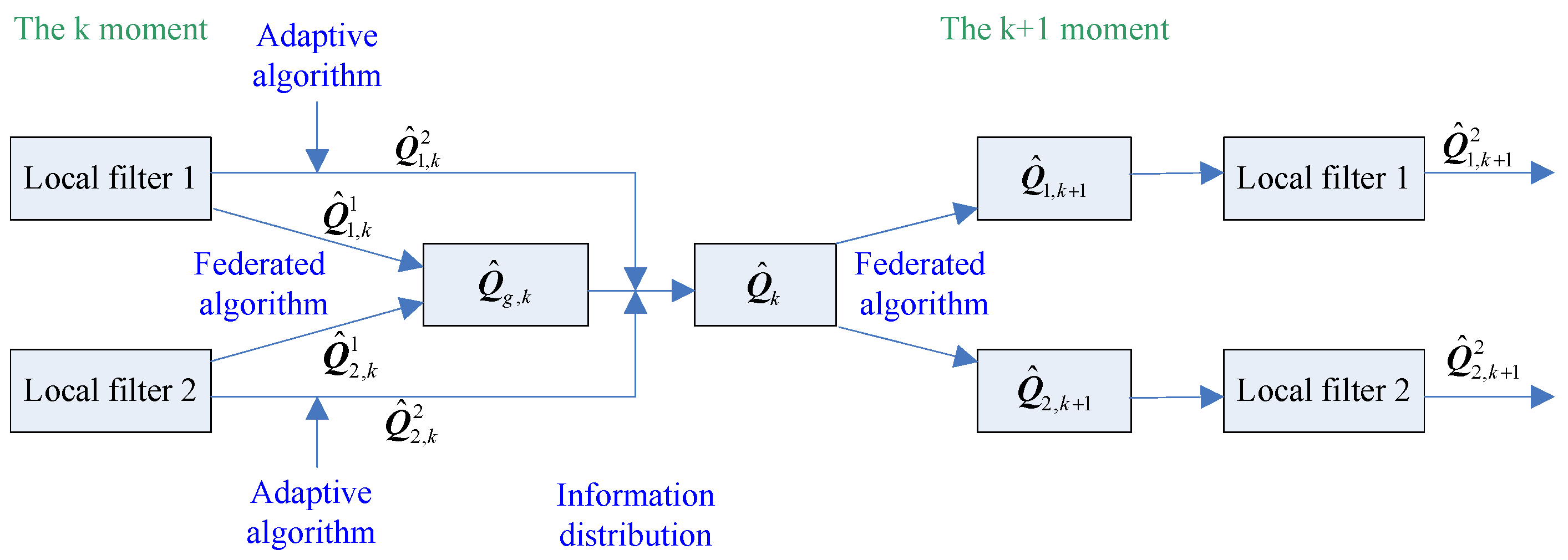
In this paper, for multi-source navigation with time-varying or mis-estimated state noise, the federated adaptive Kalman filter is used for the operation, that is, the local filters adopt the simplified Sage–Husa adaptive algorithm [
8], while, in the overall framework, the federated principle is used for calculations. In view of the fact that both the federated and the adaptive algorithm have updating principles of the state noise covariance, this paper proposes a weighting method to fuse these two principes. As a result, the federated adaptive updating process can adjust the state noise covariance according to the information distribution factor, so that the global filter can maintain stability on the basis of the adaptive changes. The trend of the weighting value can be determined by analyzing the variation characteristics of the system, and the exponential function is selected to fit the system. Compared with the federated Kalman filter and the common federated adaptive Kalman filter in the simulations, it is found that the improved federated adaptive filter is better in position and speed determination, which verifies the effectiveness of the proposed method.
The contributions of this paper are as follows: the (1) SINS (strapdown inertial navigation system)/CNS (celestial navigation system)/GNSS (global navigation satellite system) integrated navigation mode is established based on the measurement data of various sensors, and federated principle is used for distributed computing; (2) for the case with time-varying or mis-estimated state noise, federated Sage–Husa adaptive filter is chosen as the sub-filter’s algorithm, and the state noise covariance is weighted according to the federated and the adaptive principle to ensure the adaptability and stability of the global filter; (3) In the simulation part, the comparison of the navigation accuracy among federated filter, federated adaptive filter and the improved federated adaptive filter is completed.
The following chapters are structured as follows:
Section 2 introduces the principle of federated Kalman filter, including the structure and operation principle of it, as well as the algorithm of the filter.
Section 3 introduces the Sage–Husa adaptive Kalman filter algorithm.
Section 4 introduces the principle of the improved federated adaptive filter, including the selection process of the federated distribution factors and the adaptive weighting of the state noise covariance.
Section 5 constructs the SINS/CNS/GNSS integrated navigation model and gives the state equations and measurement equations of the integrated navigation;
Section 6 demonstrates the effectiveness of the improved federated adaptive filter through the simulations;
Section 7 is the conclusions.
2. Introduction of the Federated Kalman Filter
When the navigation process involves three or more navigation methods, it is difficult to combine the measurement information of each method effectively by using a single filter. For this situation, the researchers have proposed a number of distributed filter methods. The standard distributed algorithm [
9] was proposed, which is intended to establish the relationship between the distributed and centralized filter; considering the unknown correlation of local estimations, there is the covariance crossover algorithm [
10] as well as the federated algorithm [
11].
Federated Kalman filter is a special form of distributed Kalman filter and it was proposed by Carlson in the United States in 1998. It consists of several local filters and one main filter, and it is a decentralized filter method with block estimation and a two-step cascade. It assigns dynamic state and observation information to each local filter and each local filter operates separately. The results of local filters are combined according to the information distribution factors to obtain the result of the global filter. Obviously, the key of the operation lies in the information distribution process.
2.1. Principle and Structure of the Federated Kalman Filter
The federated filter operation process utilizes the measurement information of each subsystem and the common reference system for parallel independent operations. Suppose that there are
N local filters, the subscript of the main filter is
m, and the subscript of the global filter is
g, the state and measurement equations of each local filter and the main filter are as follows:
where
is the state vector of the local filter or main filter,
is the measurement vector,
is the state transition matrix of the
local filter at time
;
is the measurement matrix;
and
are the state noise matrix and measurement noise matrix of the local filter respectively, and they are all Gaussian white noise matrices, the variances are
and
respectively. It should be noted that the main filter has no measurement equation, i.e., when
, only the state equation works.
Suppose that the local optimal estimation
and its corresponding covariance
are obtained at time
, and these local optimal estimations are fused in the global filter according to the optimal fusion estimation algorithm to obtain the global optimal estimation
and its variance
. The state noise covariance matrices of the local filter and the global filter are
and
respectively, and
and
are amplified by
times and then fed back to the local filters for parameter reset, i.e., the parameter value of
k time is obtained:
where
is the information distribution factor. In addition, according to the principle of information conservation, the information distribution factor
needs to satisfy:
At the same time, the federated filter has the following principles of information distribution:
Through the above equations, the federated filter links each local filter with the main filter, and realizes the fusion process through information distribution, and different federated modes can be obtained by setting different information distribution factor
[
12]. The improved federated filter reset method proposed in this paper uses Equations (
2) and (
4) to complete the information fusion process through the allocation and addition of global filter and local filter without the participation of the main filter.
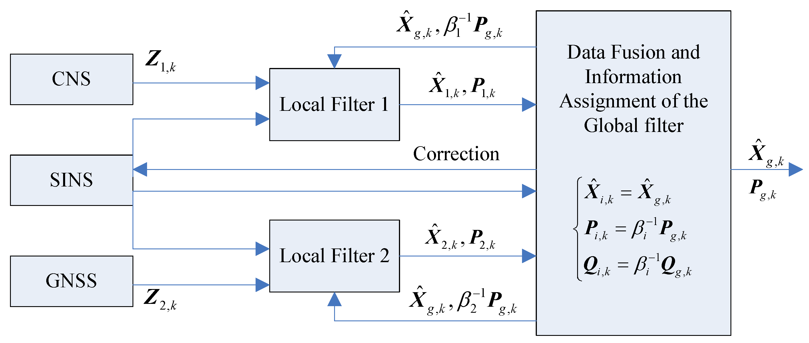
For the integrated navigation of SINS, CNS and GNSS in this paper, two local filters are set—SINS/CNS local filter 1 and SINS/GNSS local filter 2, each of which is independent in data processing. As for the setting of the main filter, it is necessary to consider the actuality of the system. For this system, in the case that the initial state noise estimation is not accurate or the state noise is time-varying, the main filter is not accurate without the measurement equation, so the main filter can be left. The data of each navigation subsystem is input to the corresponding local filter, and the output is the result of information fusion, and the global filter result can be obtained, then the global state estimation is realized. The structure of the federated filter is as
Figure 1:
As can be seen from
Figure 1, on the one hand, the information from the global filter is output to the outside, and, on the other hand, it is fed back to each sub-filter. The existence of the feedback process makes the information fusion process of the distributed filter more efficient and accurate.
2.2. Algorithm Flow of the Federated Kalman Filter
For the federated filter structure without the main filter (i.e.,
), parameters and their changes of the local filter affect the result of the global filter [
13]. Taking the discrete model in Equation (
1) as an example, the steps of the federated filter algorithm are mainly as follows:
a. Initialization:
Firstly, global estimation initialization is performed, and the initial value of the state vector , the initial value of the state covariance , and the initial value of the state noise are known.
b. Information distribution (reset):
Secondly, the information distribution process is as follows:
In this process, the value of
affects the proportion of each local filter, and the principles of subsystems are not the same as each other. The specific selection principle is described in
Section 4.1:
c. Local estimation:
The state measurement is updated:
d. Global integration:
After each round of the filter calculation process, it will return to the information distribution (reset) link to start the next round of calculation.
3. Introduction of the Sage–Husa Adaptive Filter
The Sage–Husa algorithm is an adaptive filter algorithm based on the statistical characteristics of the system [
14]. For the case that the statistical properties of the state and measurement noise are unknown, the maximal posterior estimation principle can be used to obtain the estimated value [
15] to improve the filter accuracy. The estimation algorithm is suitable for general linear time-varying systems. The recursive calculation process is simple and suitable for many fields.
Consider the mathematical model of the linear discrete systems:
where
is the state transition matrix;
is the measurement matrix;
and
are the state noise matrix and the measurement noise matrix, and the covariance matrices are
and
, respectively, and their statistical properties are unknown.
For the systems where the variance
of measurement noise is time-varying or unknown, the general Kalman filter algorithm is difficult to meet the accuracy requirements of the system due to the lack of updating procedures for the system and measurement noise. From the aspect of optimizing the filter performance, the contribution rate of the new data to the filter can be correspondingly improved, so the operator
is needed, satisfying
where
b is the forgetting factor, and
. The corresponding iterative factor’s updating process is as follows:
where
and
are the estimates of the mathematical expectation of the system error and measurement error at time
k, respectively.
and
are the estimates of the variance of the system error and measurement error at time
k, respectively. Combining the above iterative factors with the Kalman filter algorithm, a robust adaptive Kalman filter algorithm which can automatically track noise can be obtained as follows:
The one-step prediction equation:
The mean square error of the one-step prediction:
The estimation of the mean square error:
By adjusting the forgetting factor b, the adaptive process of the system can be fulfilled.
6. Simulation and Analysis
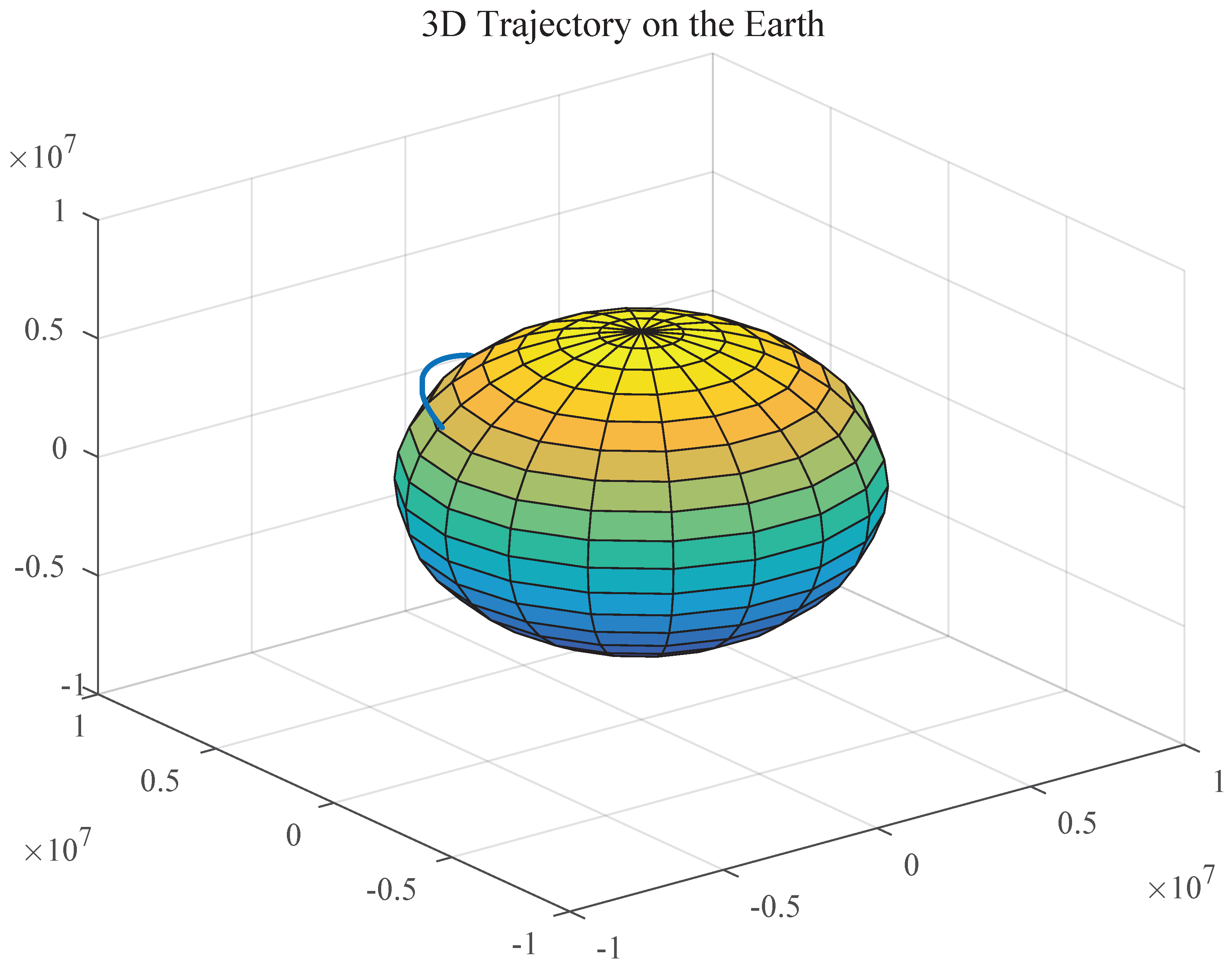
Assume that the trajectory of the aircraft is shown in
Figure 3:
Assume that the basic simulation conditions are: The random drift of SINS gyro is 0.5°/h. The random offset of accelerometer is 50 g; Initial misalignment angle is . Initial state noise covariance estimation is unbiased, which is , and , , where g is the acceleration of gravity; the initial position of the aircraft is of east longitude, of north latitude; the shooting angle is ; the thrust acceleration is 40 m/s at the first 60 s; in the launch inertial system, the initial pitching angle is and remains the same during the first 10 s, then it changes from to in the form of quadratic function during the next 50 s, and then it remains the same during the rest of the time; in addition, the heading angle and rolling angle are both throughout the whole process; the simulation time is 1110 s, the sampling interval is 0.01 s, and 50 Monte Carlo simulations are performed.
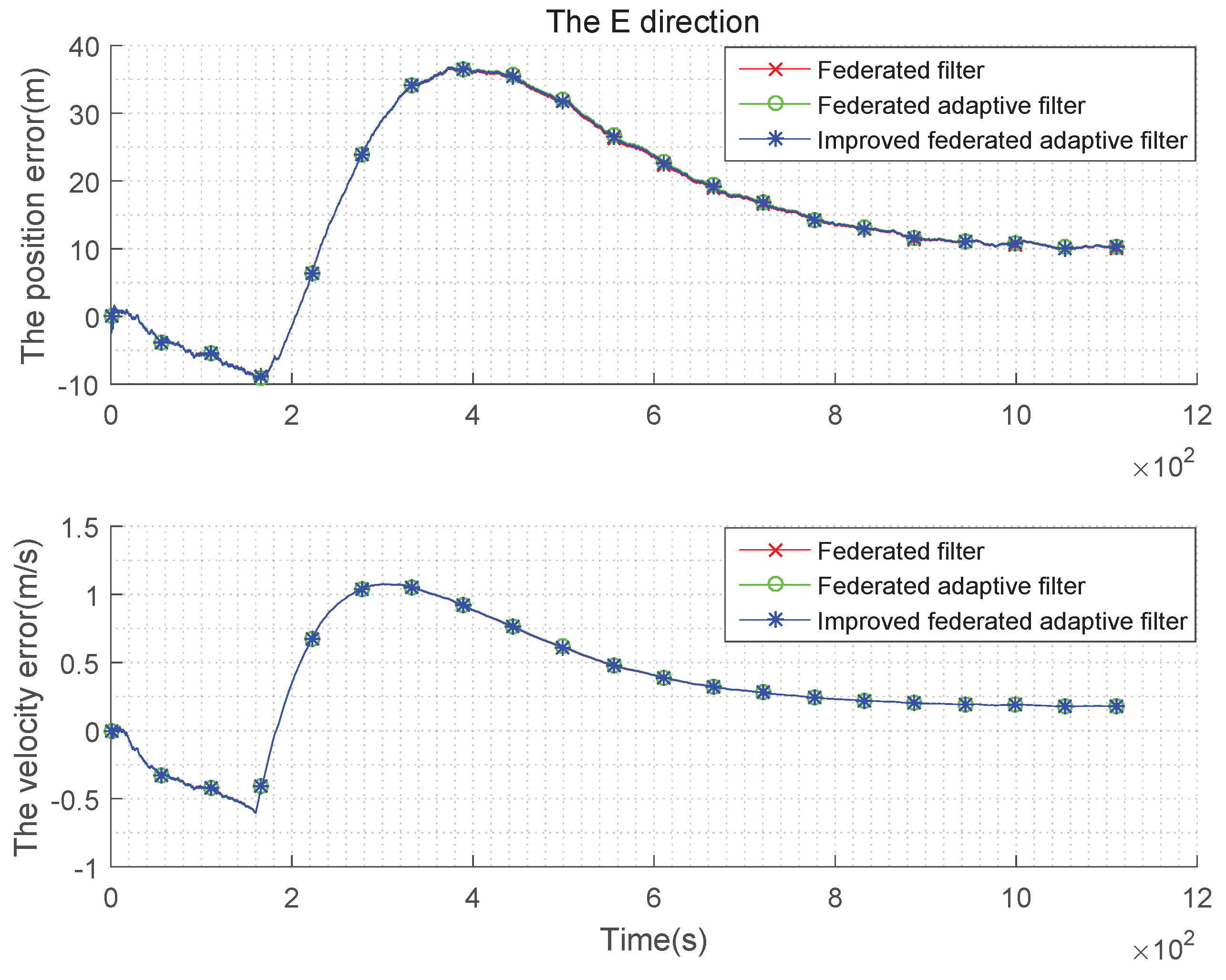
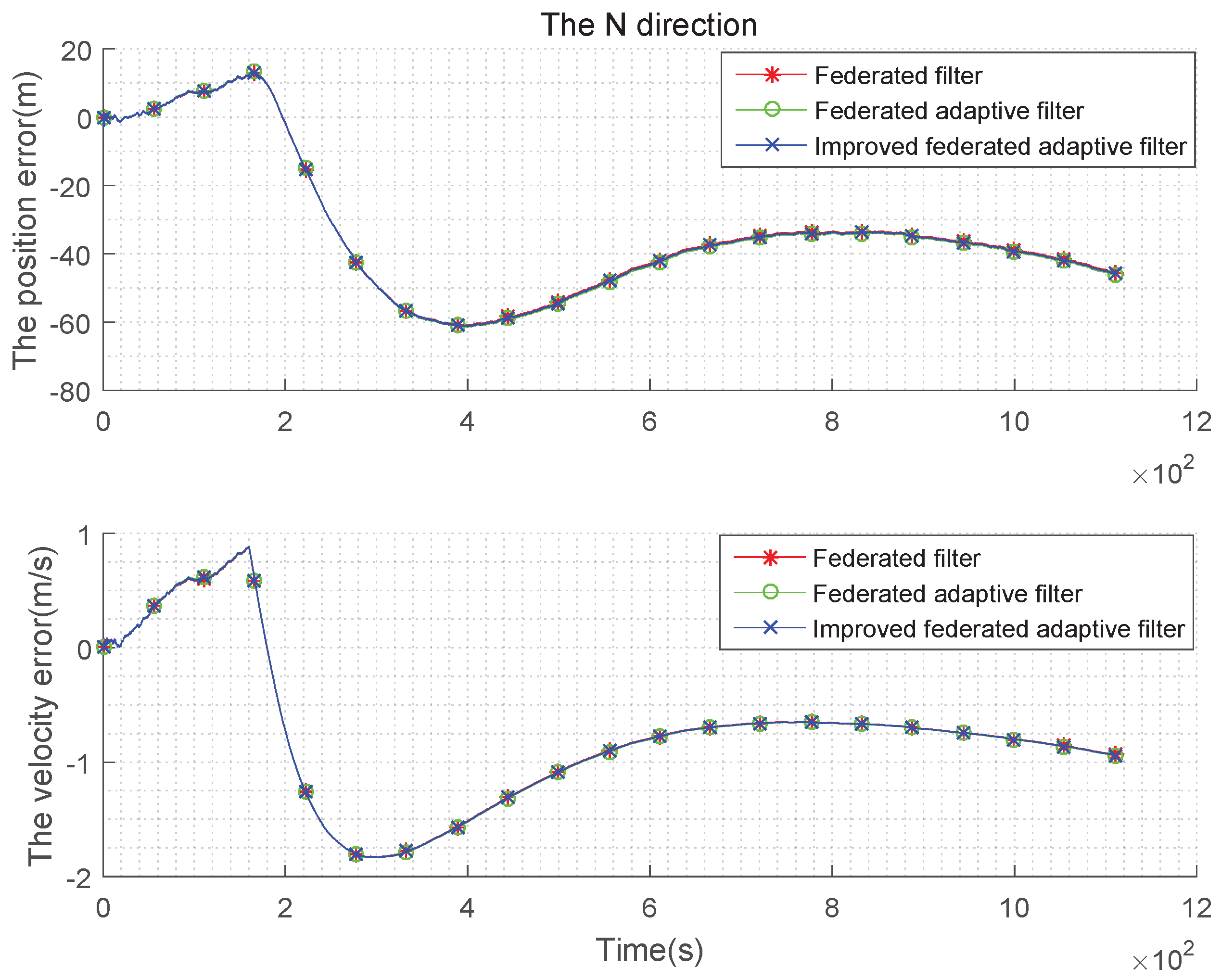
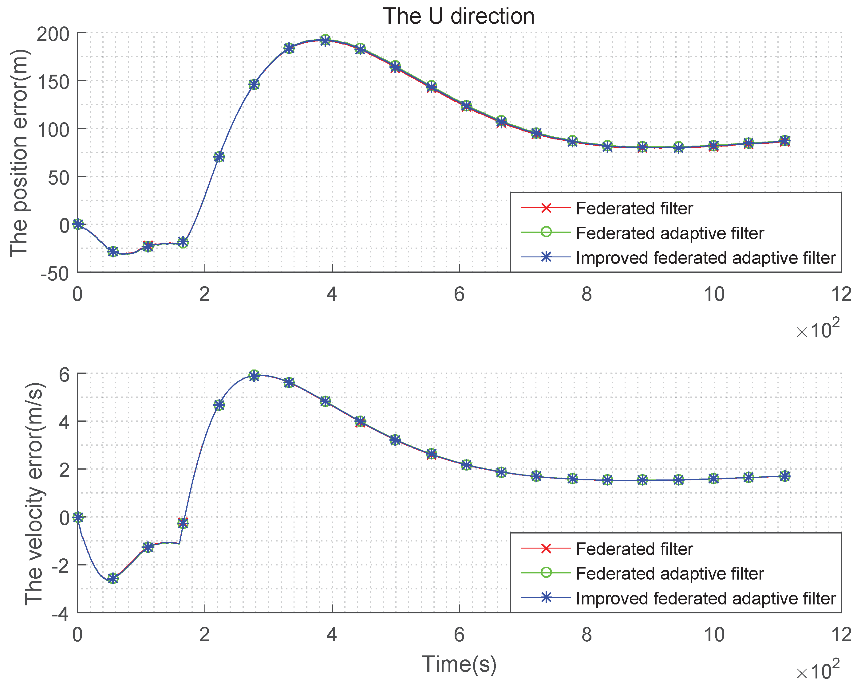
(1) Gaussian state noise and the estimation are unbiased:
The condition setting with Gaussian state noise and unbiased estimation is the same as the basic simulation conditions above. Taking the average of the errors, the improved federated Sage–Husa adaptive filter, federated Sage–Husa adaptive filter and the federated filter are used in integrated navigation, and the simulation error curves are shown in the
Figure 4,
Figure 5 and
Figure 6:
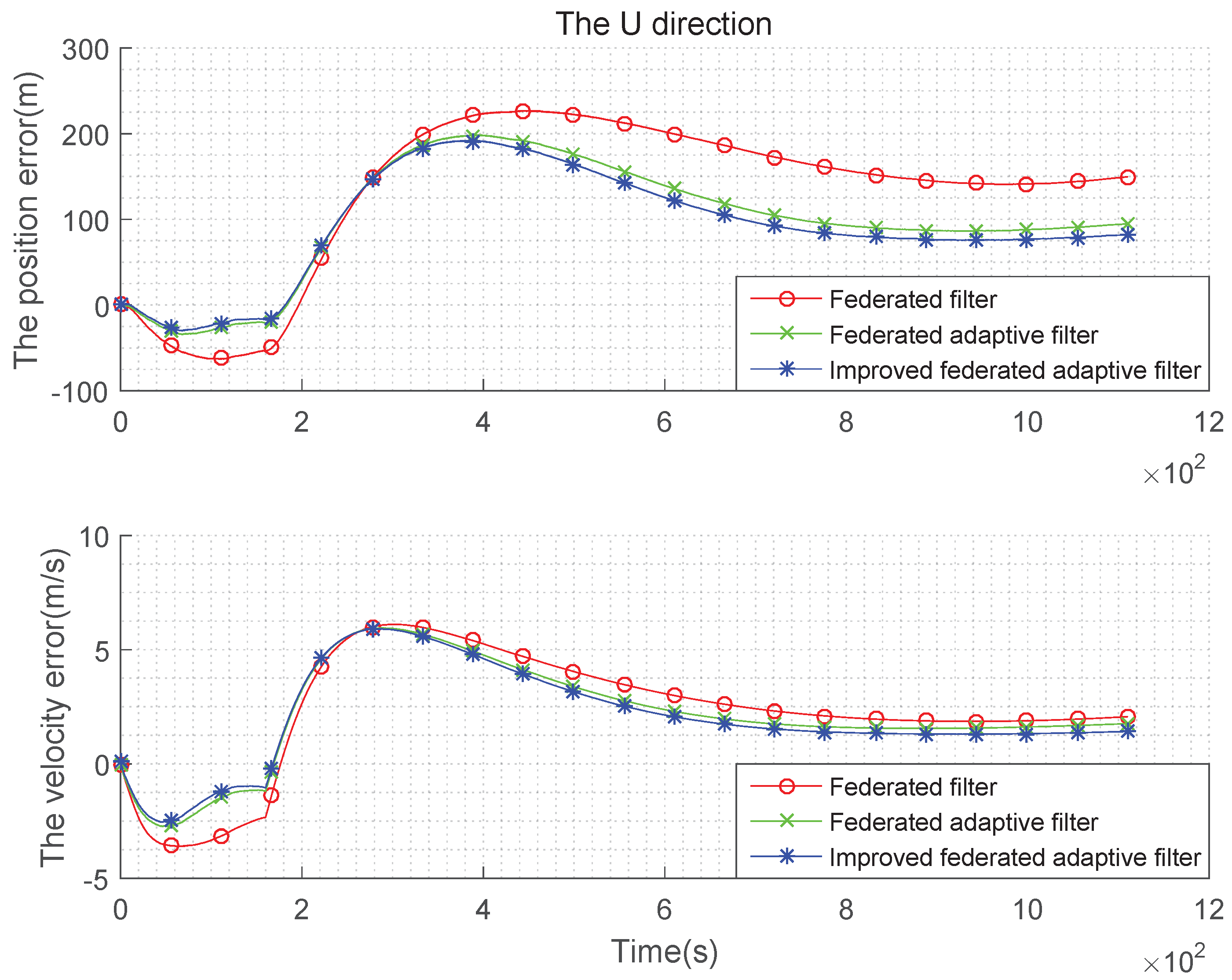
It can be seen from the
Figure 4,
Figure 5 and
Figure 6 that there are almost no differences in the navigation errors of the three methods in the three directions. The following table is a quantitative analysis.
It can be seen from the
Table 1 and
Table 2 that the navigation errors of the three methods in three directions are almost the same, and the subtle differences are too small to be noticed, that is, when the state noise is Gaussian and the estimation is unbiased, the three methods are roughly the same.
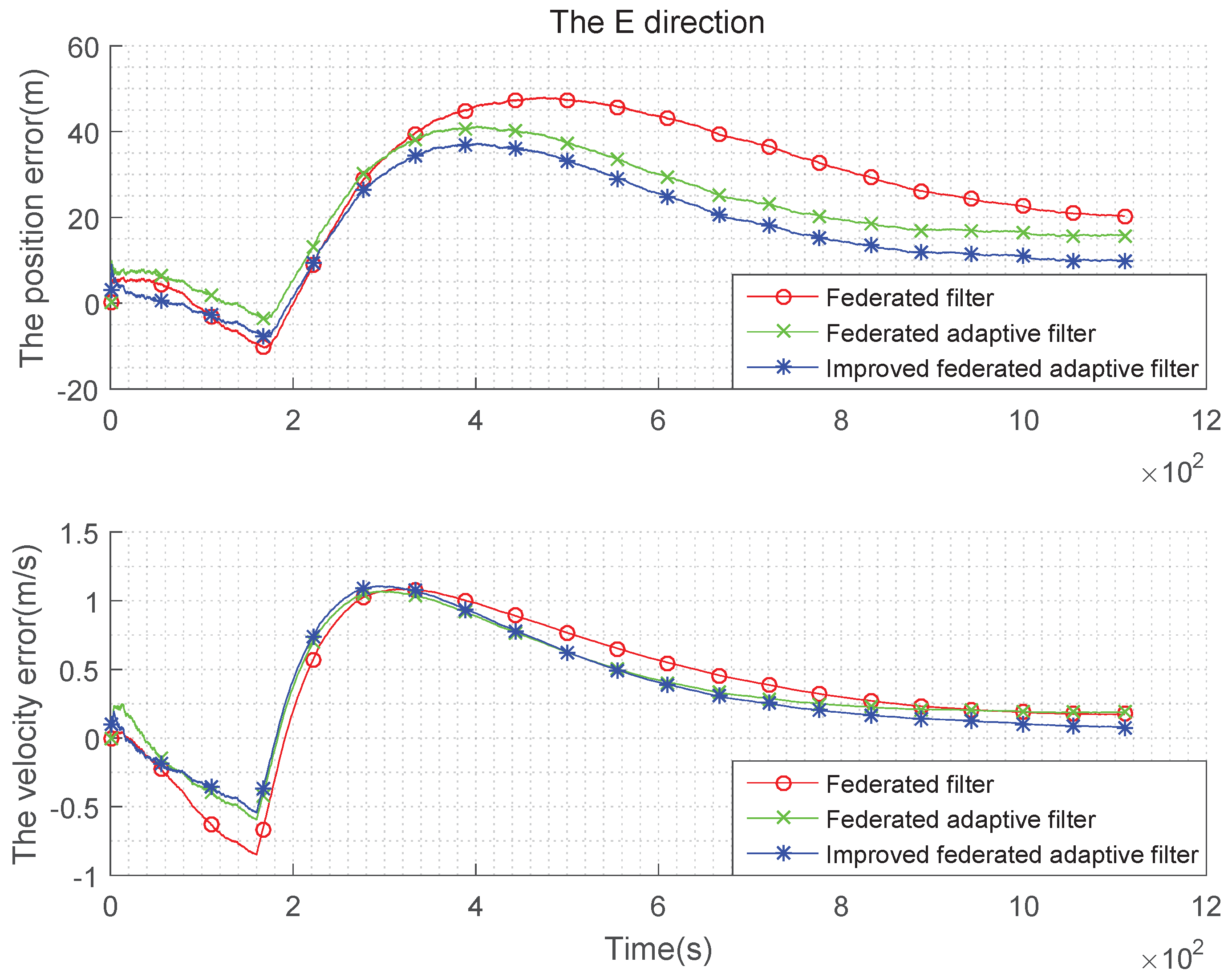
(2) Gaussian state noise and the estimation are biased:
The settings of the parameters are same as those in Tabel (1), and the initial estimation of state error covariance is .
It can be seen from the above
Figure 7,
Figure 8 and
Figure 9 and the
Table 3 and
Table 4 that, when the estimation of the state noise is deviated, even if the state noise is Gaussian, the filter effects of the three methods are different. In the comparison of position and velocity errors, the improved federated adaptive filtering is the best, followed by the federated adaptive filter, the federated filter is not effective because it depends on the initial value of the state noise.
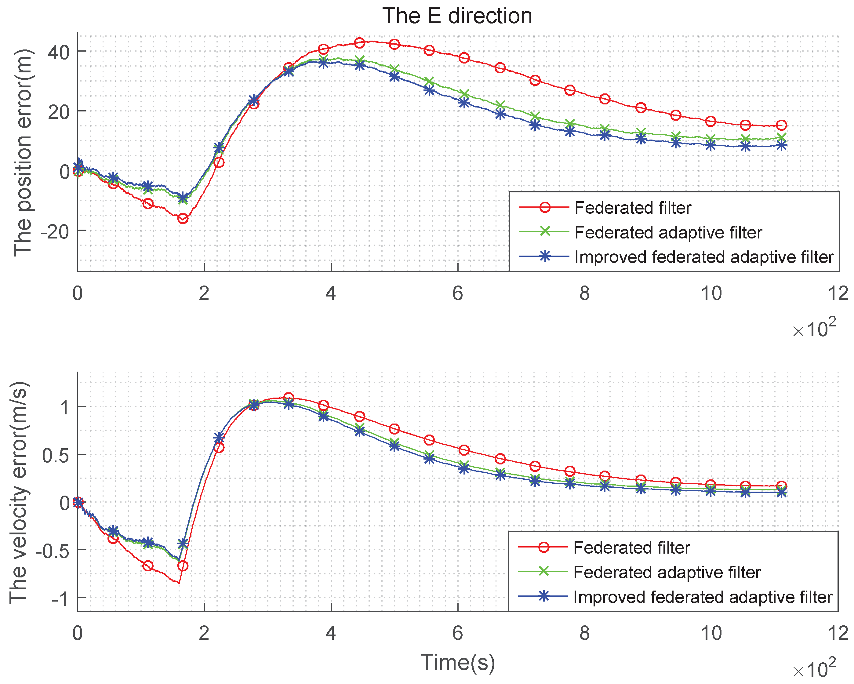
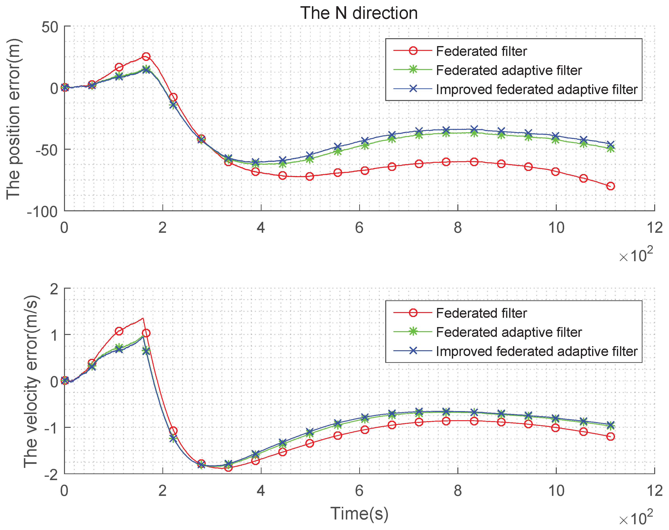
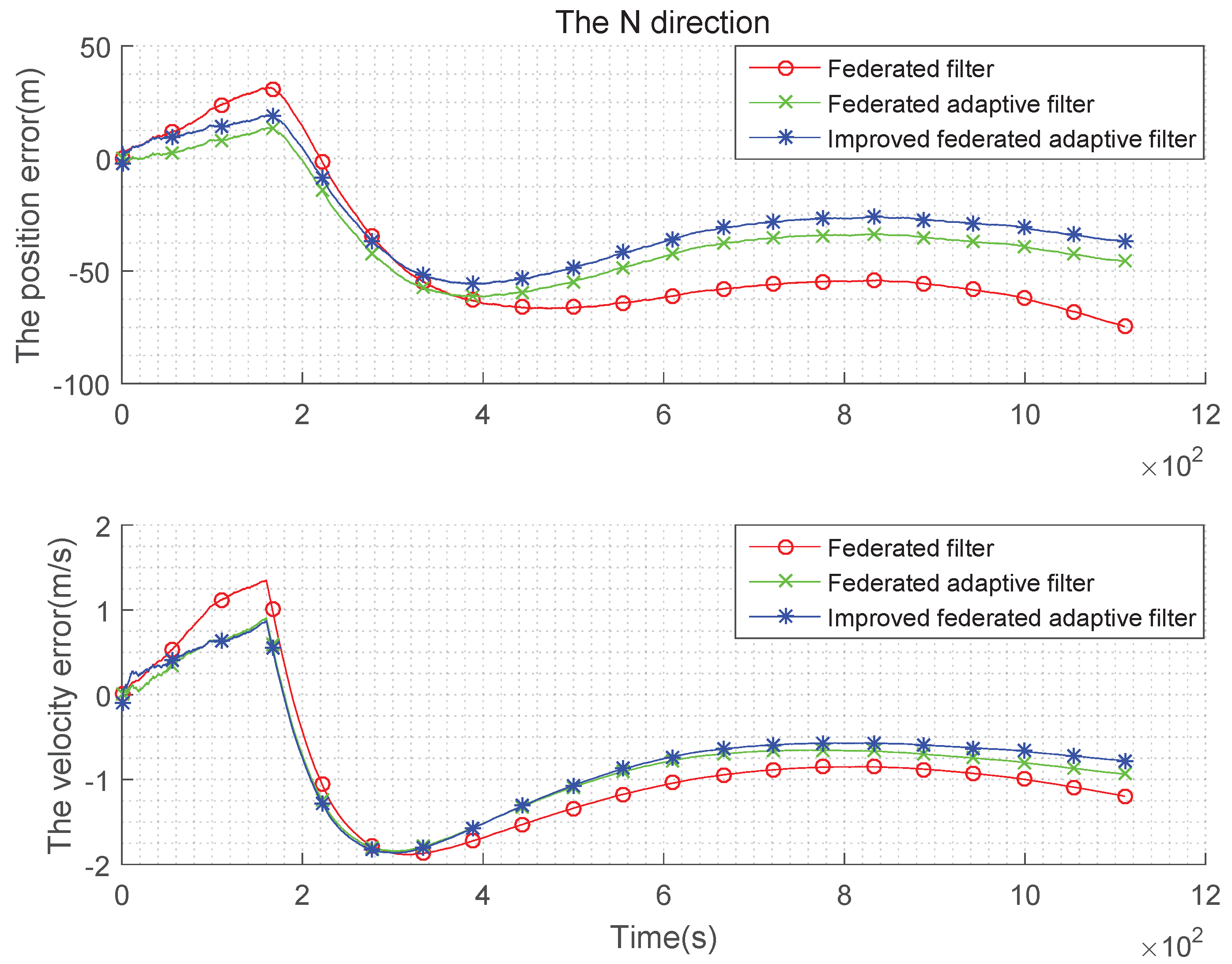
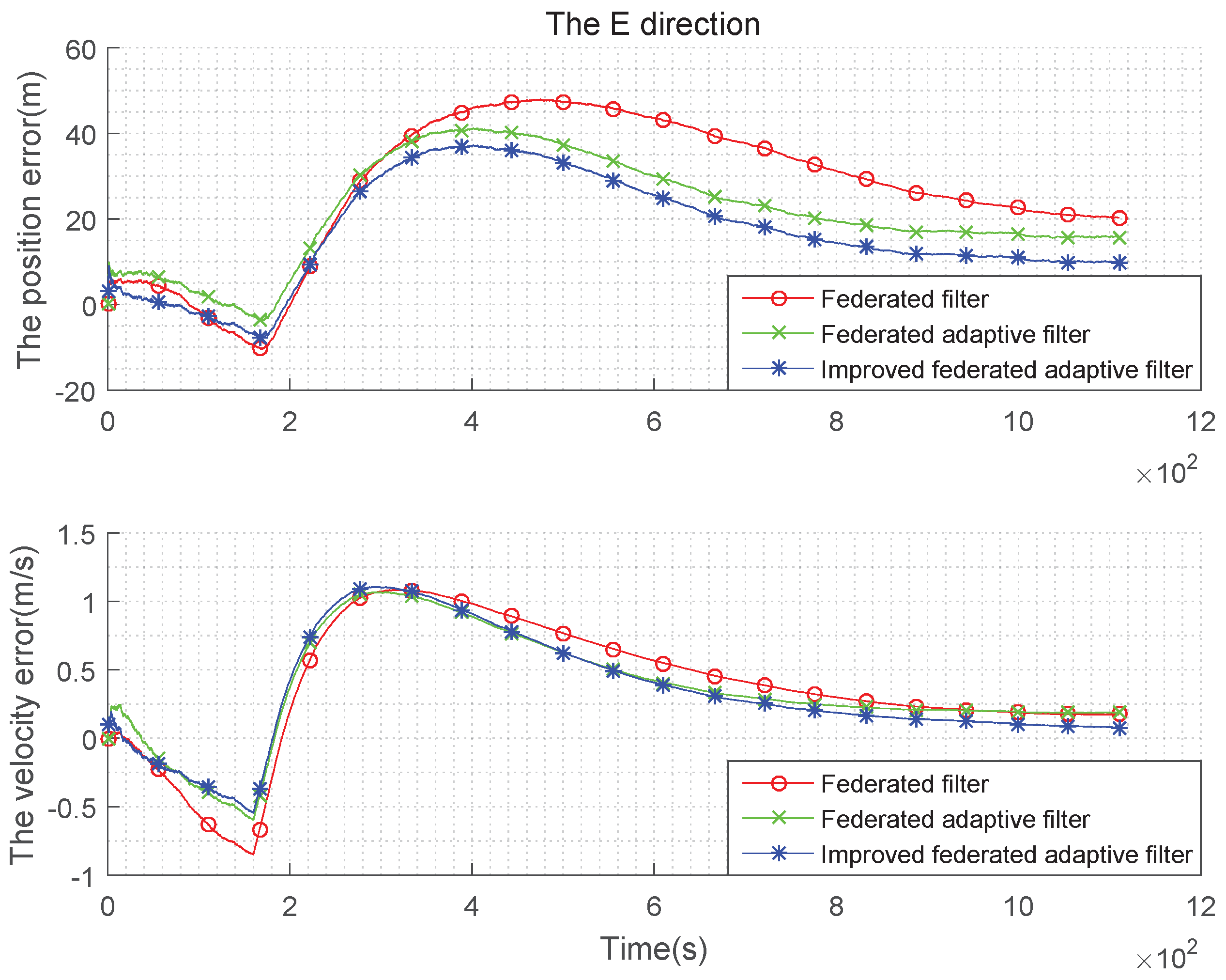
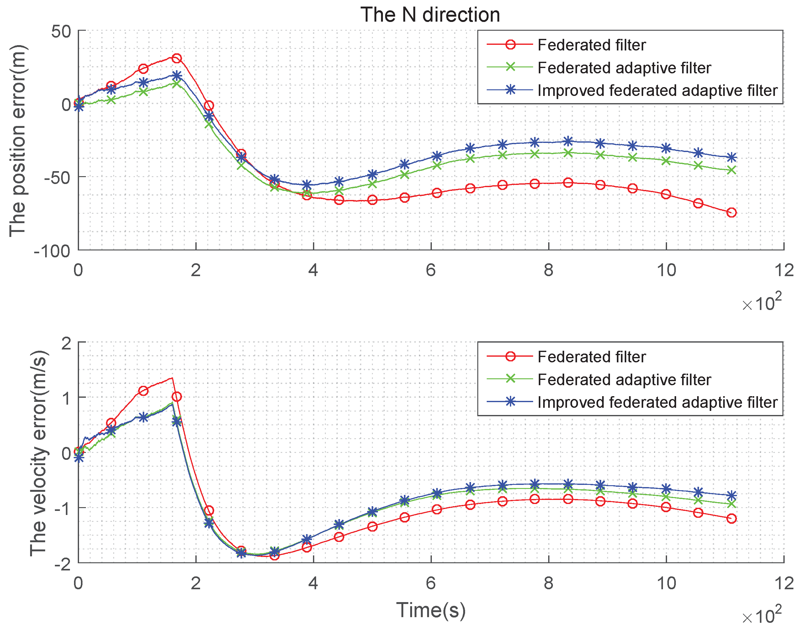
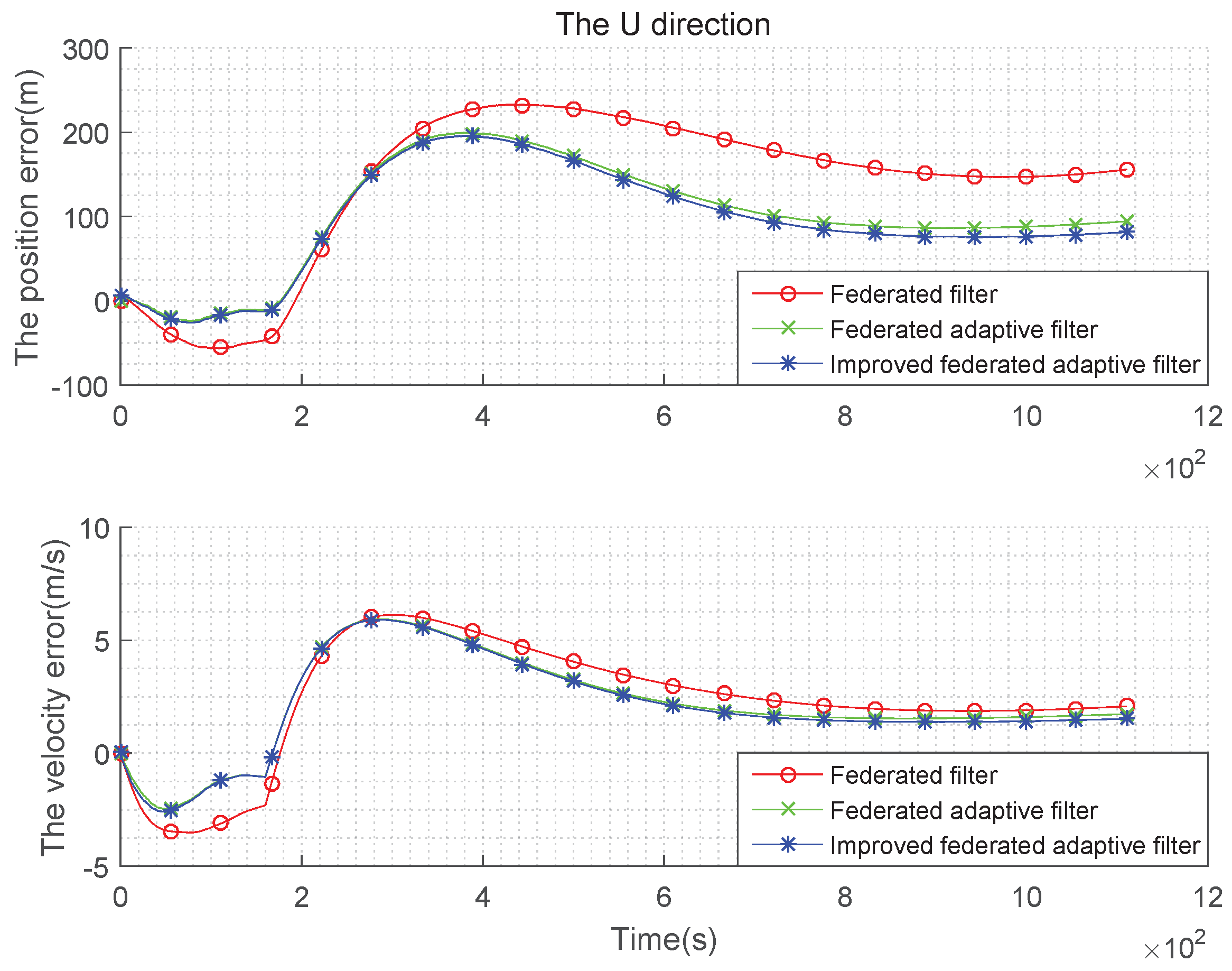
(3) Non-Gaussian state noise and the estimation are biased:
In the test (2), the setting of the parameters is added as follows: The SINS gyro random constant drift is 0.2°/h, the accelerometer’s random offset is 50
g, and the initial misalignment angle is
. The simulation error curve is shown in the
Figure 10,
Figure 11 and
Figure 12:
The above simulation is performed under the condition that the state noise is non-Gaussian and the estimation is biased, the tables are obtained in the case of using the federated Kalman filter, the federated adaptive filter and the improved federated adaptive filter to compare speed with position error in three directions. It can be seen from
Figure 10,
Figure 11 and
Figure 12 that, in the initial time, the three methods have large fluctuations owing to too few samples. As the number of samples increases, the three methods get stable gradually. In addition, when the number of samples increases to a certain extent, the advantages of improved federated adaptive filter gradually appear, which is the best among the three methods, while the federated adaptive method is the second, and the federated Kalman filter is the worst. The error statistics in three directions are shown in
Table 5 and
Table 6.
It can be seen from the comparison of the position and velocity errors that in the integrated navigation process, the effect of the improved federated adaptive filter is better than the other two methods in the three directions.
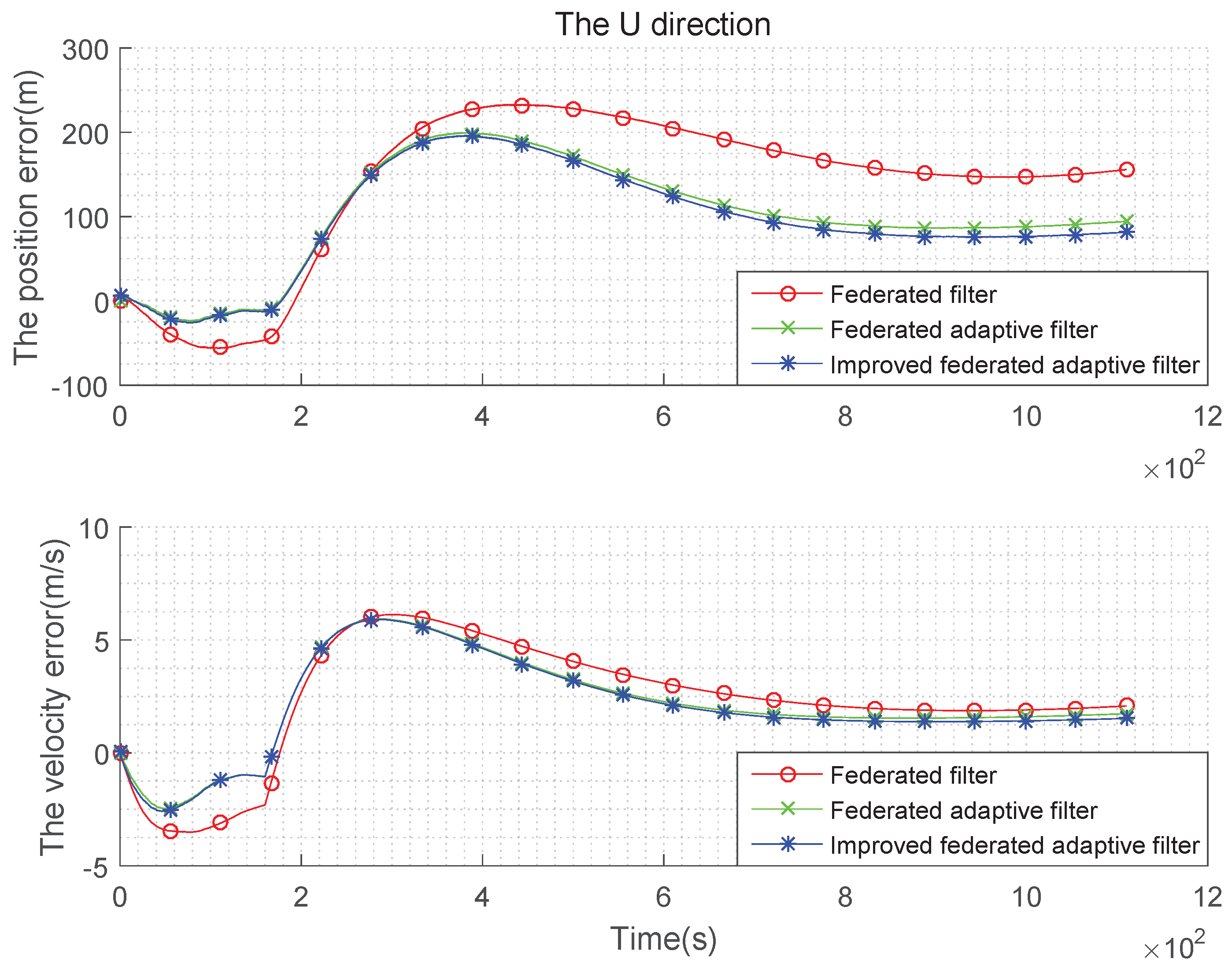
(4) Time-varying state noise and the estimation are biased:
Let the constant offset of the gyroscope in test (3) be set to 0, and it increases to 0.2°/h with time. The random offset of the accelerometer is set to 0 at the beginning, and it evenly increases to 50
g with time. The comparison of the three methods in three directions is as
Figure 13,
Figure 14 and
Figure 15:
It can be seen from the above
Figure 13,
Figure 14 and
Figure 15 and the
Table 7 and
Table 8 that, when the state noise is time-varying, the filter effect of the three methods is similar to the case of the non-Gaussian state noise. Improved federated adaptive filter has the best effect of the position and velocity error, followed by federated adaptive filter, while the federated Kalman filter is the worst.
Comparing the improved federated adaptive filter and federated filter in different situations, comparison of position error under the conditions of test (1) and test (4) can be taken as an example, and the precision changes of the two filters in E-N-U directions are shown in
Table 9.
“+” means the precision is improved, while “−” means the accuracy is reduced. It can be seen from
Table 9 that the precision of the improved federated adaptive filter has few changes for different conditions of state noise, while the federated filter’s precision decreases significantly, which shows that the improved federated adaptive filter has little dependence on the initial noise estimation, but the federated filter depends more.
Therefore, to sum up the above four cases, it can be seen that the improved federated adaptive filter algorithm can perform operations based on the state noise with unknown characteristics, and its filter accuracy is higher than the other two methods. However, since the filter algorithm designed in this paper improves the estimation of the statistical characteristics of the unknown state noise, the difference of the velocity error between the three methods is not as obvious as the position error, and it is related to the system characteristics. In summary, for different systems, the weighting mode and weighting function should be selected according to the characteristics of the system to obtain the optimal result of the federated adaptive filter.


