Capacitive Bio-Inspired Flow Sensing Cupula


Abstract
:1. Introduction
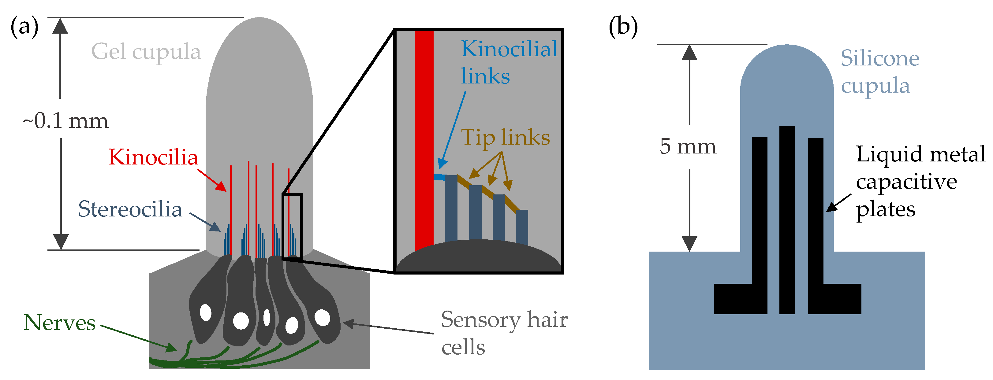
2. Design and Operating Principle
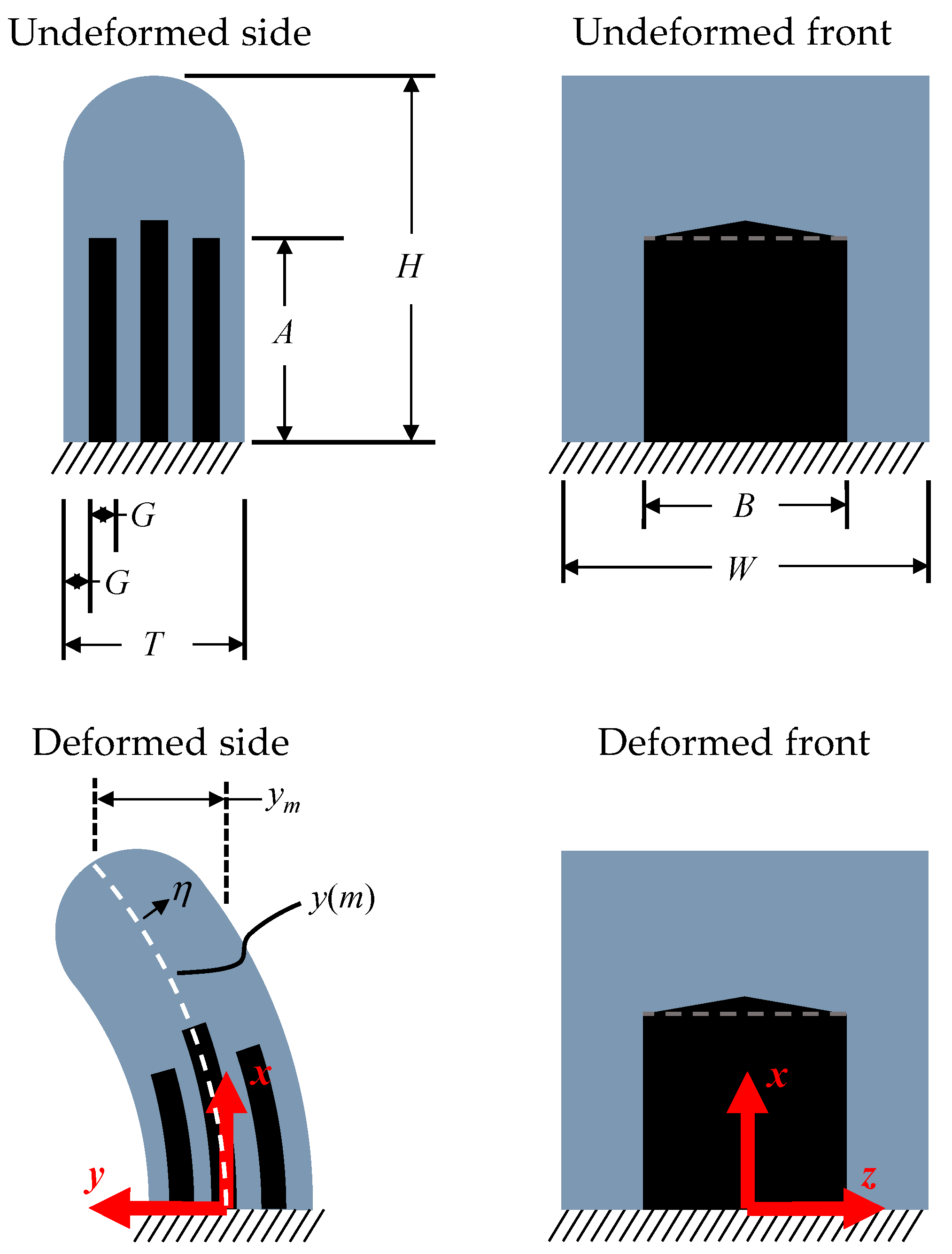
2.1. Kinematics and Capacitance
2.2. Deformation under Flow
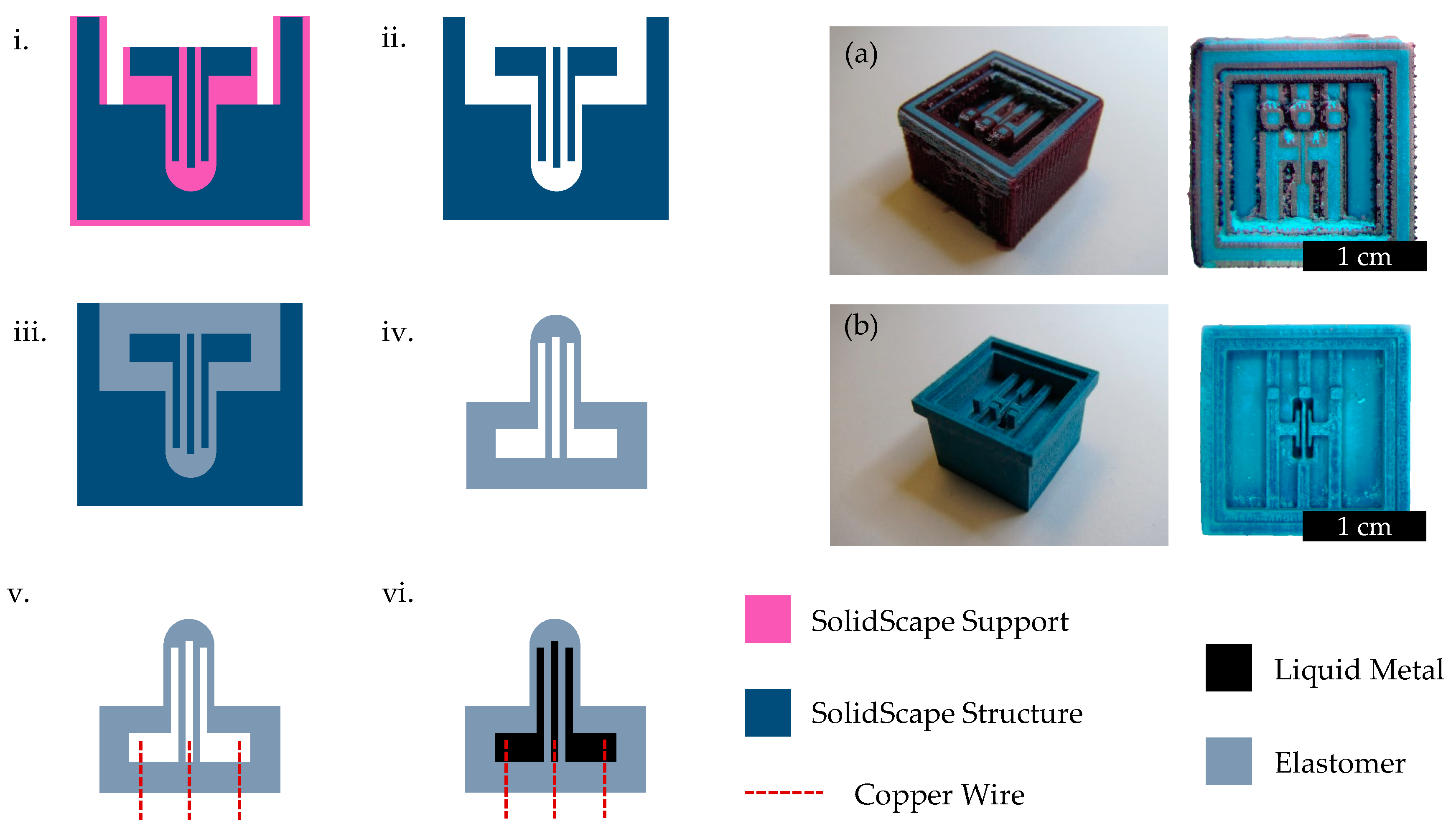
3. Fabrication
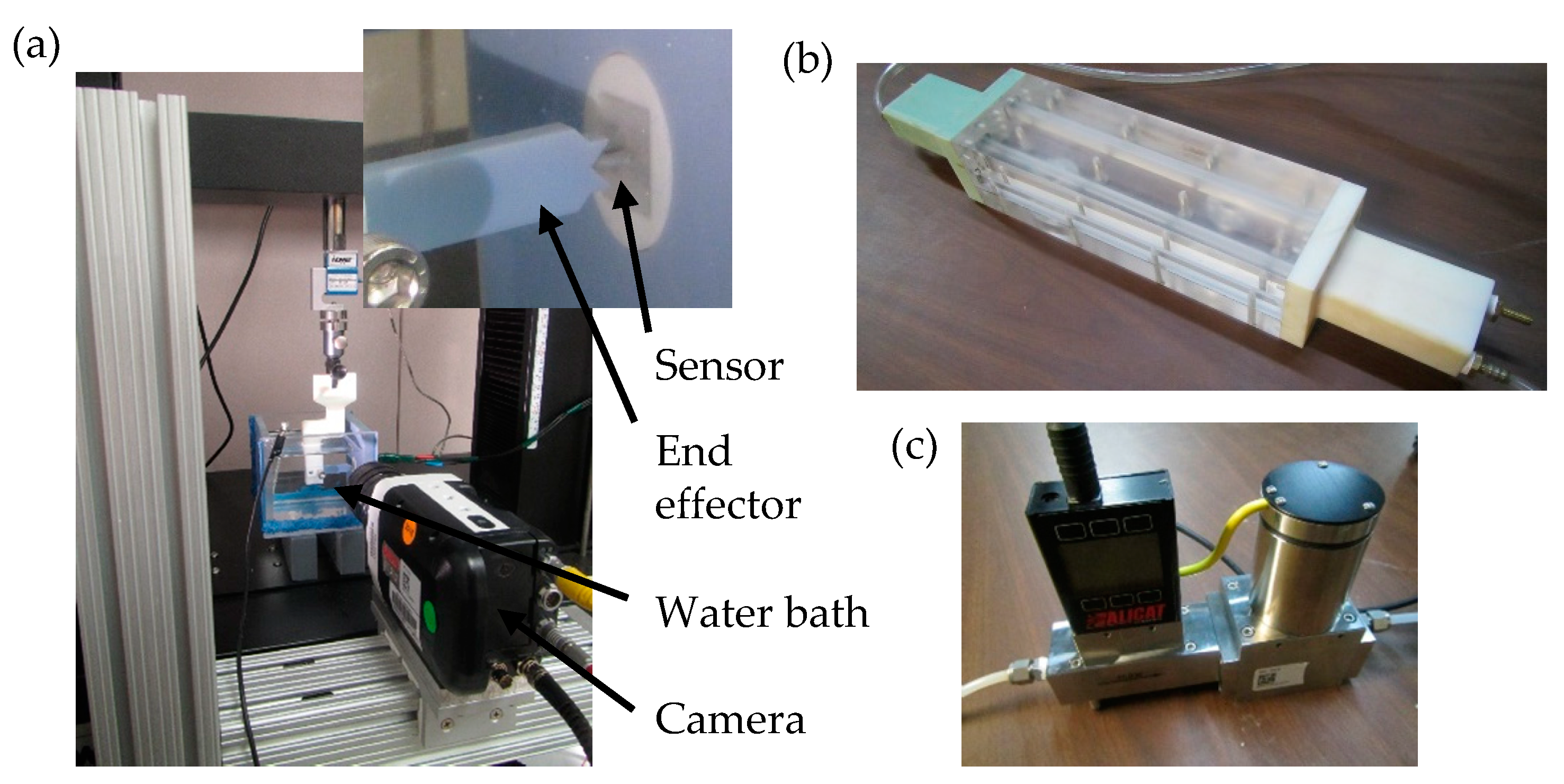
4. Experimental Setups and Methods
4.1. Cupula Displacement Testing
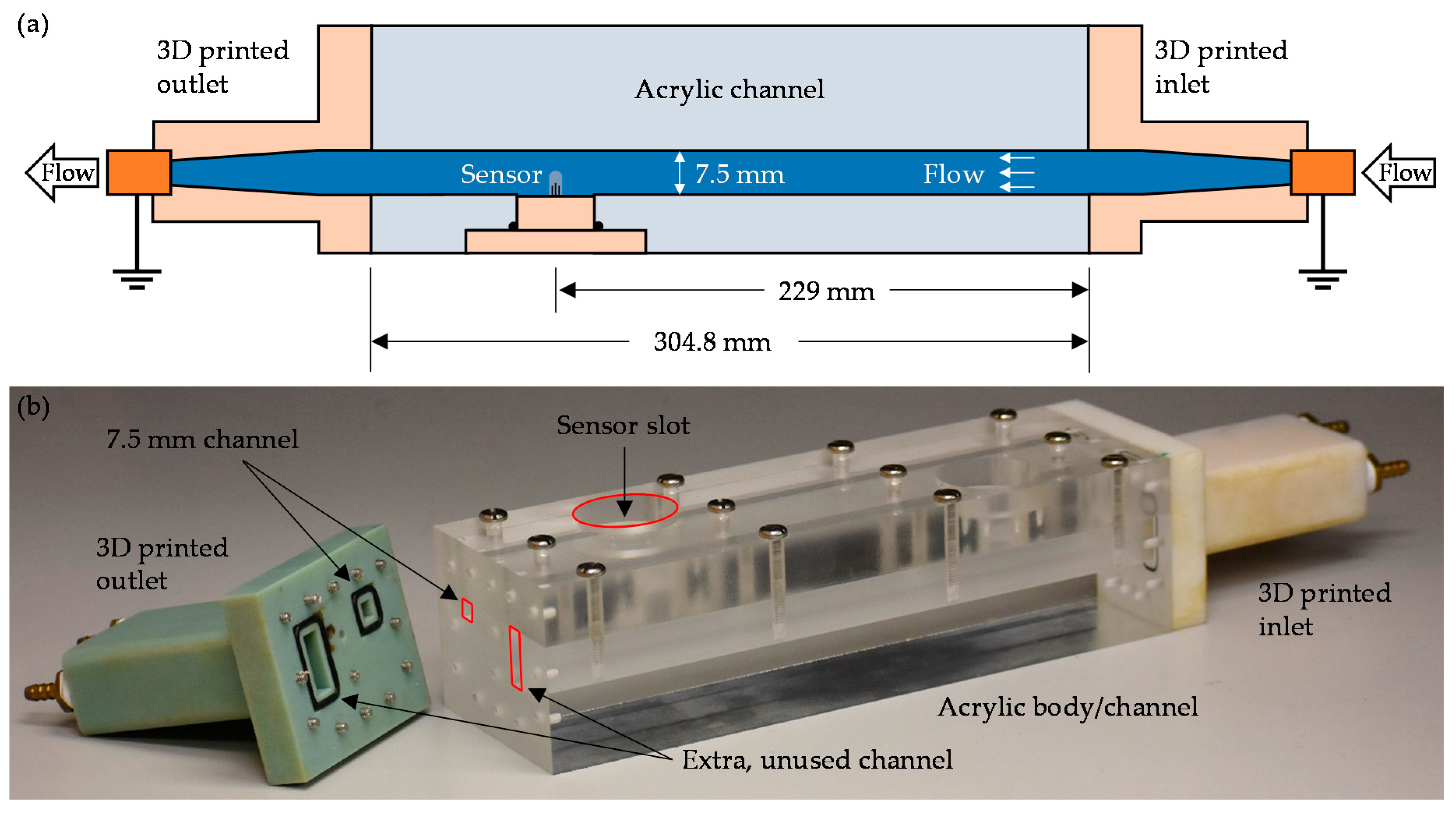
4.2. Flow Testing
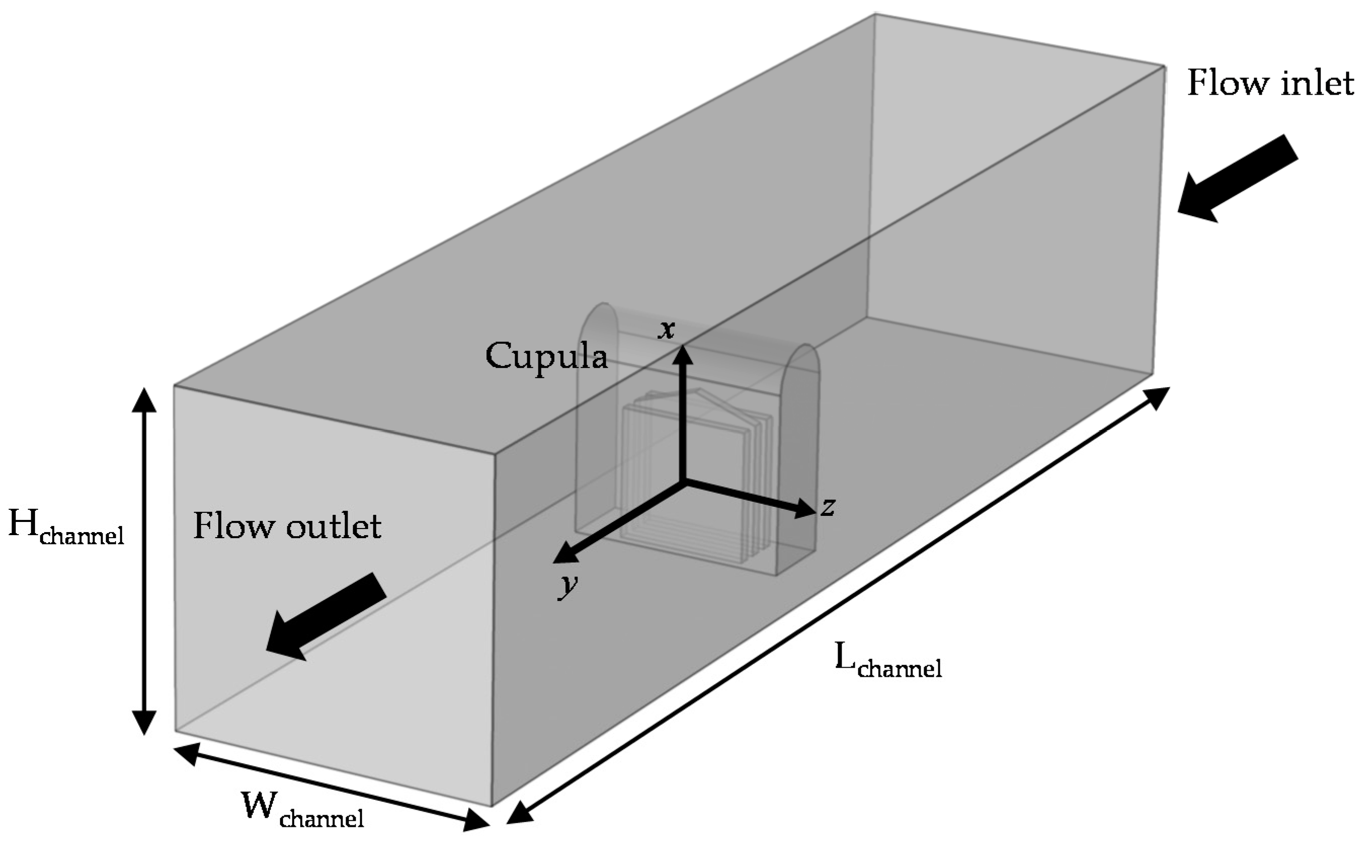
4.3. COMSOL Setup
5. Results and Discussion
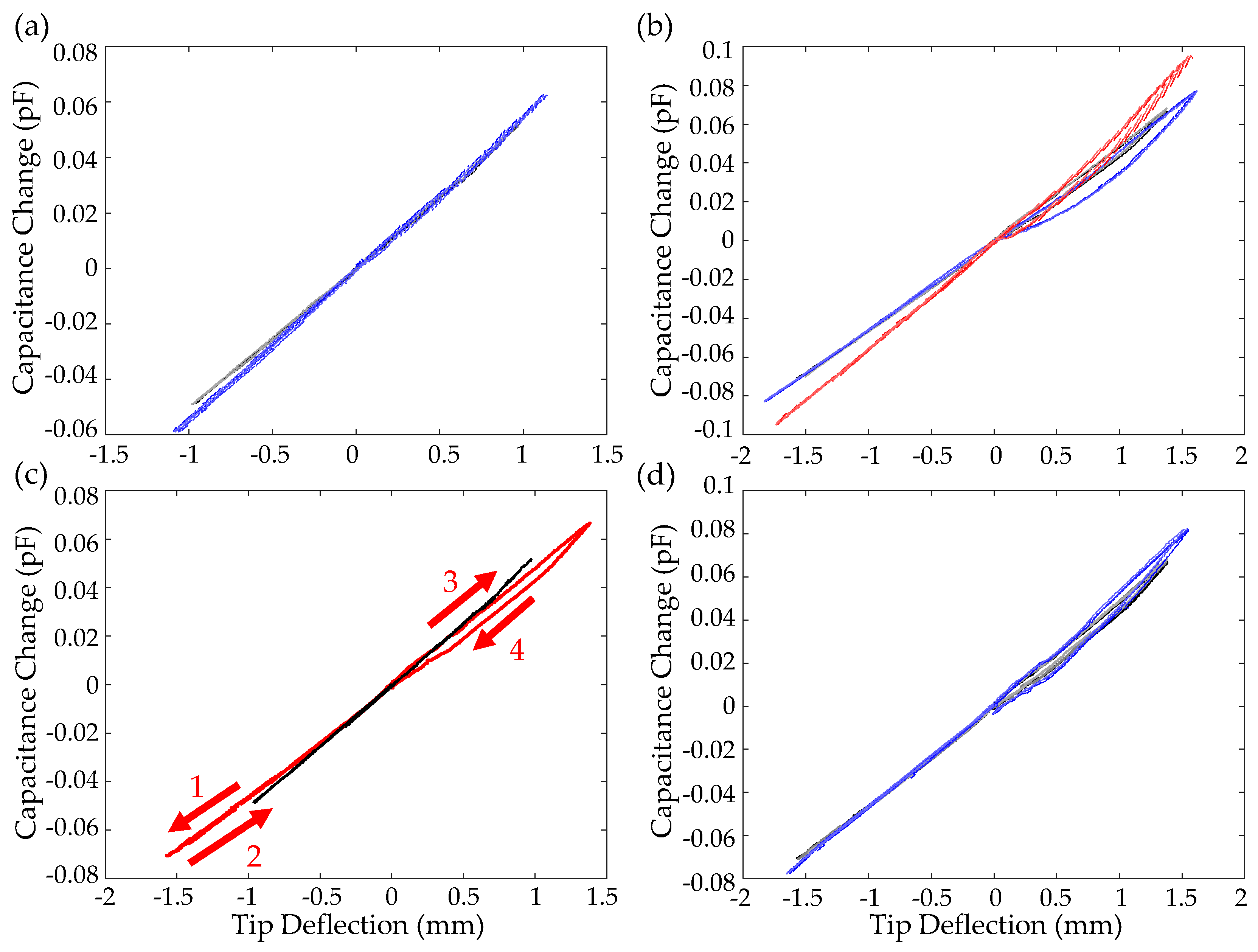
5.1. Capacitance vs. Deflection
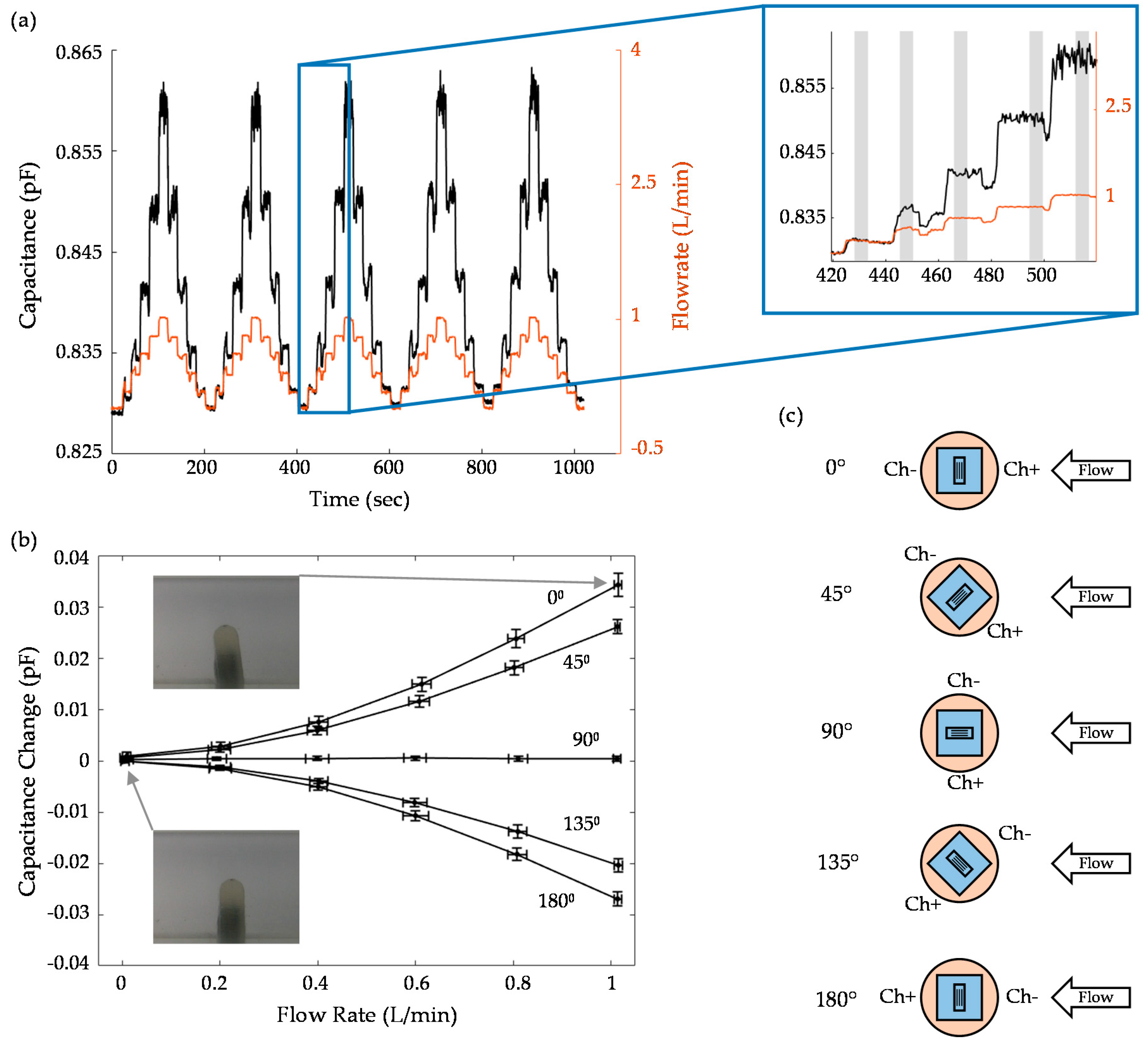
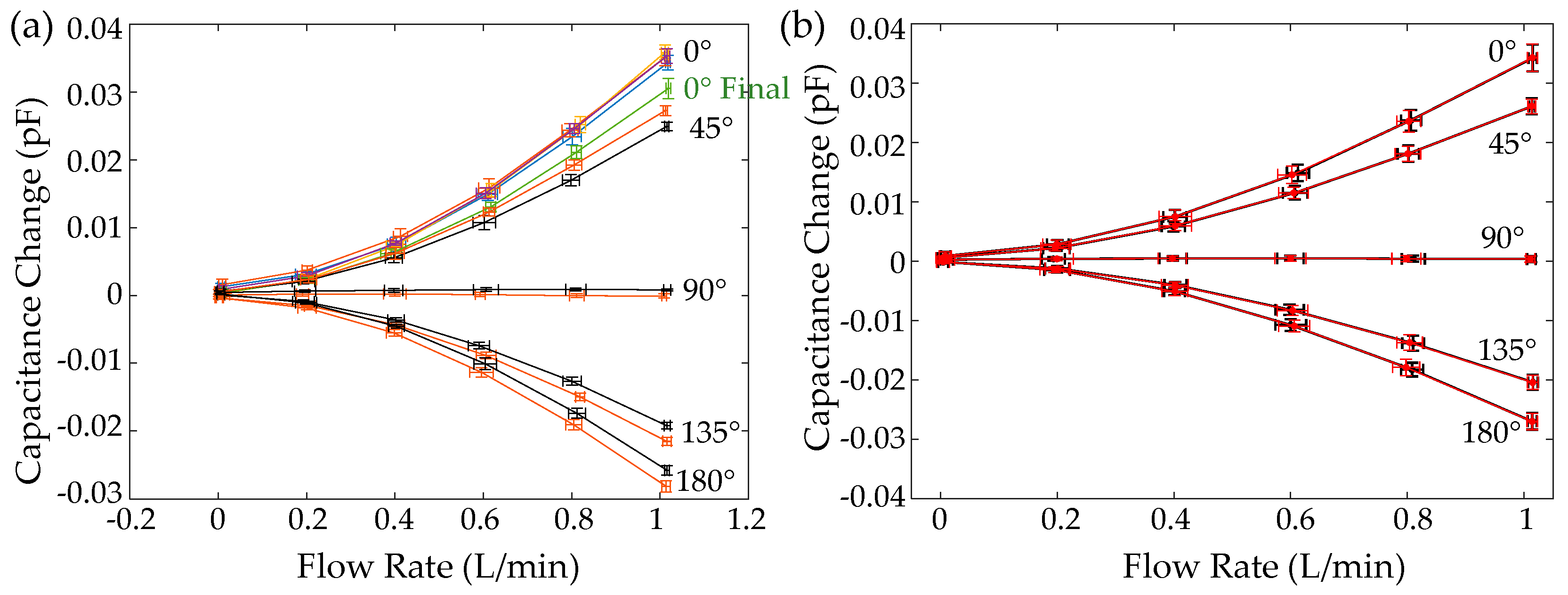
5.2. Capacitance vs. Flow
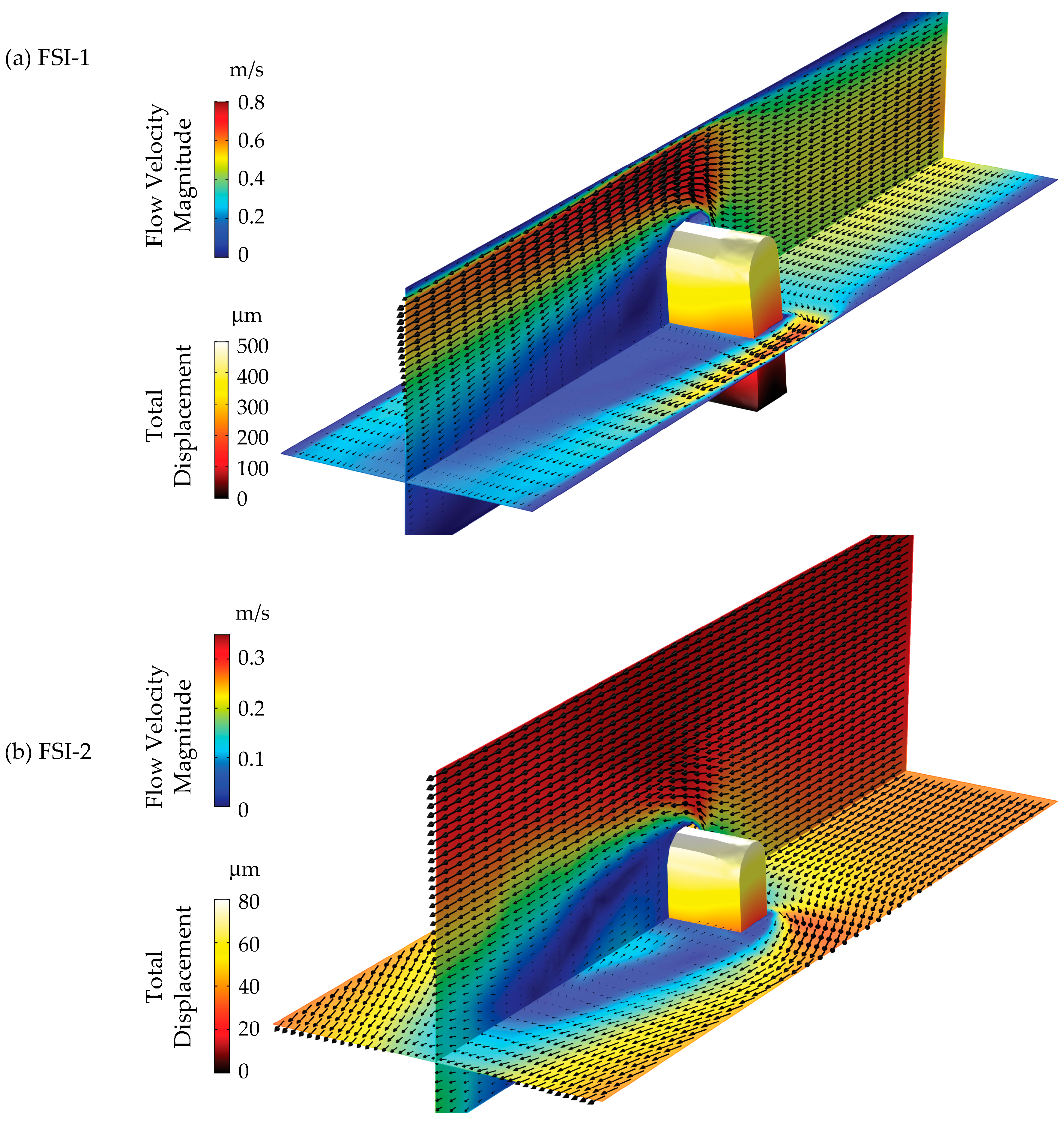
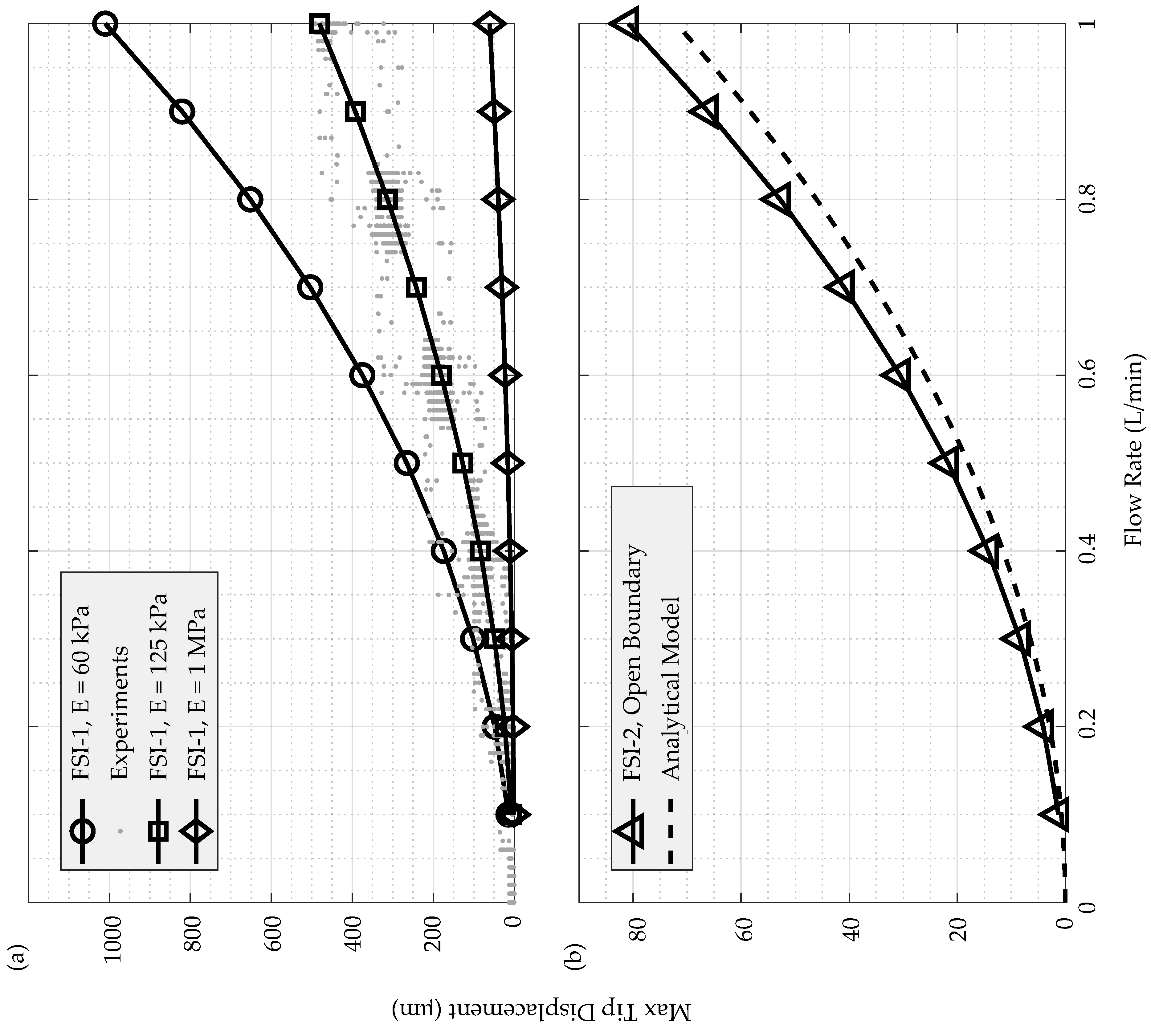
5.3. COMSOL Results
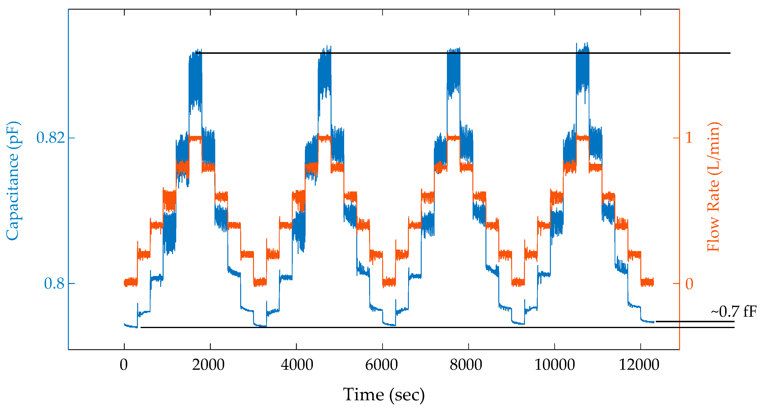
5.4. Sensing Threshold Comparison

| Source | Type | Animal/Cupula Material | Height (mm) | Aspect Ratio | Min DC (mm/s) | Min AC (mm/s) |
|---|---|---|---|---|---|---|
| [70] | Electrochemical | Xenopus Laevis | 0.1 | 3 | -- | 0.025 * |
| [71] | Electrochemical | Xenopus Laevis | 0.1 [70] | 3 [70] | -- | 0.038 |
| [6] | Electrochemical | Cheimarrichthys fosteri | 0.036 [72] ** | -- | 5 | -- |
| [6] | Electrochemical | Pagothenia borchgrevinki | -- | -- | 20 | -- |
| [6] | Electrochemical | Astyanax fasciatus | 0.104 [16] | 4 [16] | 30 | -- |
| [19] | Piezoresistive | SU-8 | 0.6 | 7.5 | 25 | 0.7 |
| [16] | Piezoresistive | Hydrogel-capped SU-8 | 0.825 | 4 | -- | 0.0025 |
| [20] | Piezoresistive | Copper, gold, permalloy | 0.82 | 8.2 | 200 | -- |
| [14] | Piezoelectric | Hydrogel-capped copper | 2.7 | 0.5 | 75 | -- |
| [24] | Piezoelectric | Hydrogel-capped PDMS *** | 1.5 | 1.5 | -- | 0.008 |
| [17] | IPMC **** | PDMS-capped IPMC | 35 | 5 | 75 | -- |
| [30] | Optics | Silicone | 3 | 4.3 | 70 | 0.004 |
| [28] | Capacitive | Epoxy | 40 | 20 | 100 | -- |
| This work | Capacitive | Liquid metal, silicone | 5 | 1 | 60 | -- |
6. Conclusions
Author Contributions
Funding
Acknowledgments
Conflicts of Interest
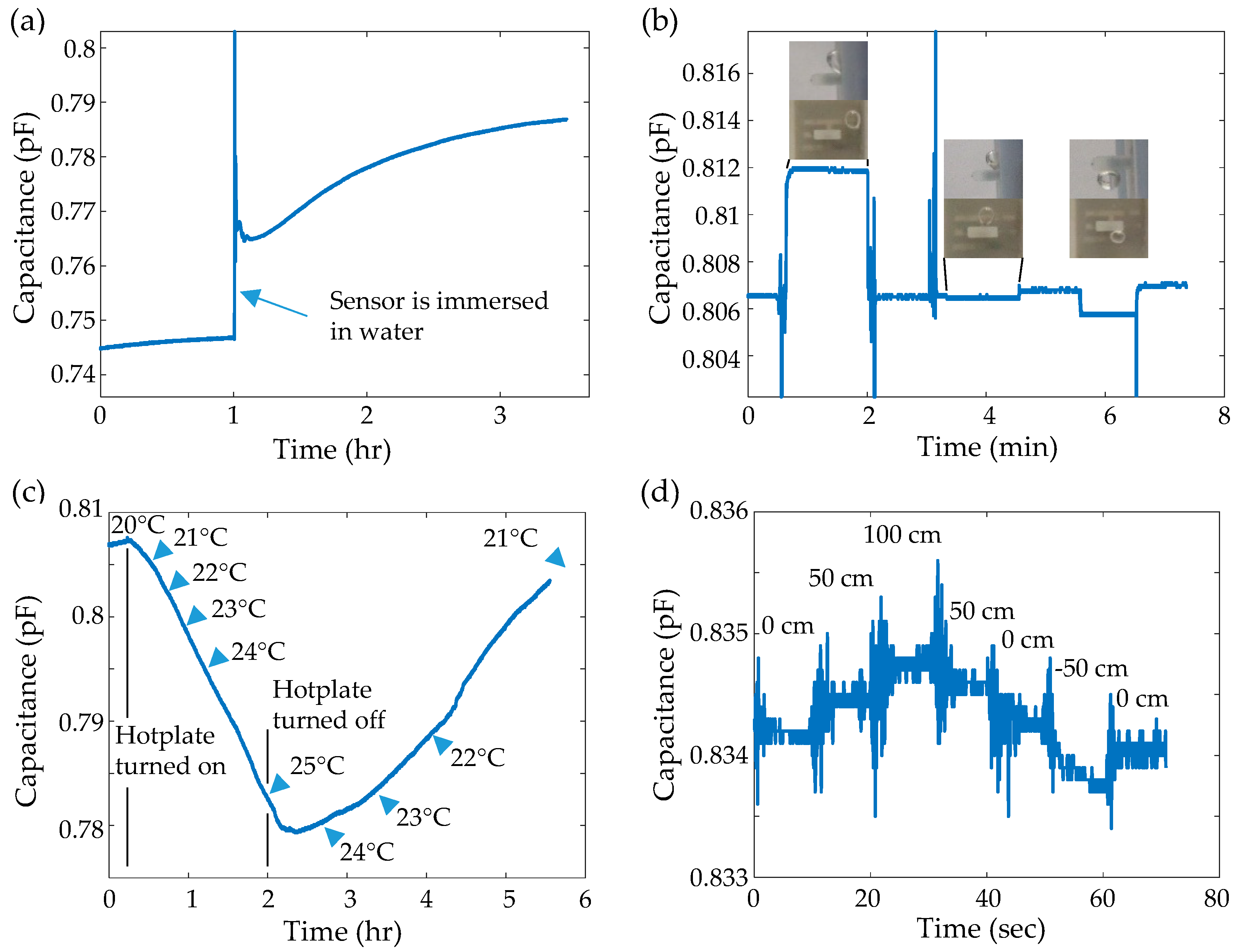
Appendix A. Sensor Drift

Appendix B. Additional Direct Deflection Data

Appendix C. Additional Flow Data


Appendix D. Experimental Setup Images

References
- Barrett, D.S.; Triantafyllou, M.S.; Yue, D.K.P.; Grosenbaugh, M.A.; Wolfgang, M.J. Drag reduction in fish-like locomotion. J. Fluid Mech. 1999, 392, 183–212. [Google Scholar] [CrossRef] [Green Version]
- Geder, J.D.; Ramamurti, R.; Pruessner, M.; Palmisano, J. Maneuvering Performance of a Four-Fin Bio-Inspired UUV. In Proceedings of the 2013 OCEANS, San Diego, CA, USA, 23–27 September 2013. [Google Scholar]
- Sfakiotakis, M.; Lane, D.; Davies, J. Review of fish swimming modes for aquatic locomotion. IEEE J. Ocean. Eng. 1999, 24, 237–252. [Google Scholar] [CrossRef]
- Dean, B.; Bhushan, B.; Nosonovsky, M. Shark-skin surfaces for fluid-drag reduction in turbulent flow: A review. Philos. Trans. R. Soc. A Math. Phys. Eng. Sci. 2010, 368, 4775–4806. [Google Scholar] [CrossRef] [PubMed]
- Videler, J.J.; Weihs, D. Energetic advantages of burst-and-coast swimming of fish at high speeds. J. Exp. Boil. 1982, 97, 169–178. [Google Scholar]
- Montgomery, J.C.; Baker, C.F.; Carton, A.G. The lateral line can mediate rheotaxis in fish. Nature 1997, 389, 960–963. [Google Scholar] [CrossRef]
- Von Campenhausen, C.; Riess, I.; Weissert, R.; Campenhausen, C. Detection of stationary objects by the blind Cave FishAnoptichthys jordani (Characidae). J. Comp. Physiol. A 1981, 143, 369–374. [Google Scholar] [CrossRef]
- Liao, J.C. The role of the lateral line and vision on body kinematics and hydrodynamic preference of rainbow trout in turbulent flow. J. Exp. Boil. 2006, 209, 4077–4090. [Google Scholar] [CrossRef] [Green Version]
- Fernandez, V.I.; Maertens, A.; Yaul, F.M.; Dahl, J.; Lang, J.H.; Triantafyllou, M.S. Lateral-Line-Inspired Sensor Arrays for Navigation and Object Identification. Mar. Technol. Soc. J. 2011, 45, 130–146. [Google Scholar] [CrossRef]
- Zhang, F.; Lagor, F.D.; Yeo, D.; Washington, P.; A Paley, D. Distributed flow sensing for closed-loop speed control of a flexible fish robot. Bioinspiration Biomimetics 2015, 10, 65001. [Google Scholar] [CrossRef]
- McHenry, M.J.; van Netten, S.M. The flexural stiffness of superficial neuroasts in the zebrafish (Danio rerio) lateral line. J. Exp. Biol. 2007, 210, 4244–4253. [Google Scholar] [CrossRef]
- van Netten, S.M. Hydrodynamic detection by cupulae in a lateral line canal: Functional relations between physics and physiology. Biol. Cybern. 2006, 94, 67–85. [Google Scholar] [CrossRef] [PubMed]
- Kindt, K.S.; Finch, G.; Nicolson, T. Kinocilia mediate mechanosensitivity in developing zebrafish hair cells. Dev. Cell 2012, 23, 329–341. [Google Scholar] [CrossRef] [PubMed]
- Bora, M.; Kottapalli, A.G.P.; Miao, J.M.; Triantafyllou, M.S. Fish-inspired self-powered microelectromechanical flow sensor with biomimetic hydrogel cupula. APL Mater. 2017, 5, 104902. [Google Scholar] [CrossRef] [Green Version]
- Hudspeth, A.J.; Choe, Y.; Mehta, A.D.; Martin, P. Putting ion channels to work: Mechanoelectrical transduction, adaptation, and amplification by hair cells. Proc. Natl. Acad. Sci. USA 2000, 97, 11765–11772. [Google Scholar] [CrossRef] [PubMed] [Green Version]
- McConney, M.E.; Chen, N.; Lu, D.; Hu, H.A.; Coombs, S.; Liu, C.; Tsukruk, V.V. Biologically inspired design of hydrogel-capped hair sensors for enhanced underwater flow detection. Soft Matter 2009, 5, 292–295. [Google Scholar] [CrossRef]
- Lei, H.; Sharif, M.A.; Paley, D.A.; McHenry, M.J.; Tan, X. Performance inprovement of IPMC flow sensors with a biologically-inspired cupula structure. In Proceedings of the SPIE Smart Structures And Materials + Nondestructive Evaluation And Health Monitoring, Las Vegas, NV, USA, 21–24 March 2016. [Google Scholar]
- Liu, G.; Wang, A.; Wang, X.; Liu, P. A Review of Artificial Lateral Line in Sensor Fabrication and Bionic Applications for Robot Fish. Appl. Bionics Biomech. 2016, 2016, 1–15. [Google Scholar] [CrossRef] [PubMed]
- Chen, N.; Tucker, C.; Engel, J.; Yang, Y.; Pandya, S.; Liu, C. Design and Characterization of Artificial Haircell Sensor for Flow Sensing With Ultrahigh Velocity and Angular Sensitivity. J. Microelectromech. Syst. 2007, 16, 999–1014. [Google Scholar] [CrossRef]
- Fan, Z.; Chen, J.; Zou, J.; Bullen, D.; Liu, C.; Delcomyn, F. Design and fabrication of artificial lateral line flow sensors. J. Micromech. Microeng. 2002, 12, 655–661. [Google Scholar] [CrossRef] [Green Version]
- Bruinink, C.; Jaganatharaja, R.; De Boer, M.; Berenschot, E.; Kolster, M.; Lammerink, T.; Wiegerink, R.; Krijnen, G.J. Advancements in Technology and Design of Biomimetic Flow-Sensor Arrays. In Proceedings of the 2009 IEEE 22nd International Conference on Micro Electro Mechanical Systems, Sorrento, Italy, 25–29 January 2009. [Google Scholar]
- Dijkstra, M.; Van Baar, J.J.; Wiegerink, R.J.; Lammerink, T.S.J.; De Boer, J.H.; Krijnen, G.J. Artificial sensory hairs based on the flow sensitive receptor hairs of crickets. J. Micromech. Microeng. 2005, 15, S132–S138. [Google Scholar] [CrossRef]
- Izadi, N.; De Boer, M.J.; Berenschot, J.W.; Krijnen, G.J. Fabrication of superficial neuromast inspired capacitive flow sensors. J. Micromech. Microeng. 2010, 20, 85041. [Google Scholar] [CrossRef]
- Asadnia, M.; Kottapalli, A.G.P.; Karavitaki, K.D.; Warkiani, M.E.; Miao, J.; Corey, D.P.; Triantafyllou, M. From Biological Cilia to Artificial Flow Sensors: Biomimetic Soft Polymer Nanosensors with High Sensing Performance. Sci. Rep. 2016, 6, 32955. [Google Scholar] [CrossRef] [PubMed]
- Engel, J.; Chen, J.; Liu, C.; Bullen, D. Polyurethane Rubber All-Polymer Artificial Hair Cell Sensor. J. Microelectromech. Syst. 2006, 15, 729–736. [Google Scholar] [CrossRef]
- Jiang, Y.; Ma, Z.; Fu, J.; Zhang, D.; Mariani, S. Development of a Flexible Artificial Lateral Line Canal System for Hydrodynamic Pressure Detection. Sensors 2017, 17, 1220. [Google Scholar] [CrossRef] [PubMed]
- Gul, J.Z.; Su, K.Y.; Choi, K.H. Fully 3D Printed Multi-Material Soft Bio-Inspired Whisker Sensor for Underwater-Induced Vortex Detection. Soft Robot. 2018, 5, 122–132. [Google Scholar] [CrossRef] [PubMed]
- Stocking, J.B.; Eberhardt, W.C.; Shakhsheer, Y.A.; Calhoun, B.H.; Paulus, J.R.; Appleby, M. A Capacitance-based Whisker-like Artificial Sensor for Fluid Motion Sensing. In Proceedings of the IEEE Sensors 2010, Kona, HI, USA, 1–4 November 2010. [Google Scholar]
- Abdulsadda, A.T.; Tan, X. An artificial lateral line system using IPMC sensor arrays. Int. J. Smart Nano Mater. 2012, 3, 226–242. [Google Scholar] [CrossRef] [Green Version]
- Klein, A.; Bleckmann, H.; Barthlott, W.; Koch, K. Determination of object position, vortex shedding frequency and flow velocity using artificial lateral line canals. Beilstein J. Nanotechnol. 2011, 2, 276–283. [Google Scholar] [CrossRef] [Green Version]
- Amjadi, M.; Kyung, K.-U.; Park, I.; Sitti, M. Stretchable, Skin-Mountable, and Wearable Strain Sensors and Their Potential Applications: A Review. Adv. Funct. Mat. 2016, 26, 1678–1698. [Google Scholar] [CrossRef]
- Wissman, J.; Perez-Rosado, A.; Edgerton, A.; Levi, B.M.; Karakas, Z.N.; Kujawski, M.; Philipps, A.; Papavizas, N.; Fallon, D.; A Bruck, H.; et al. New compliant strain gauges for self-sensing dynamic deformation of flapping wings on miniature air vehicles. Smart Mater. Struct. 2013, 22, 85031. [Google Scholar] [CrossRef]
- Rocha, R.P.; Lopes, P.A.; De Almeida, A.T.; Tavakoli, M.; Majidi, C. Fabrication and characterization of bending and pressure sensors for a soft prosthetic hand. J. Micromech. Microeng. 2018, 28, 34001. [Google Scholar] [CrossRef]
- Park, Y.-L.; Chen, B.-R.; Wood, R.J. Design and Fabrication of Soft Artificial Skin Using Embedded Microchannels and Liquid Conductors. IEEE Sens. J. 2012, 12, 2711–2718. [Google Scholar] [CrossRef]
- Boley, J.W.; White, E.L.; Chiu, G.T.-C.; Kramer, R.K. Direct Writing of Gallium-Indium Alloy for Stretchable Electronics. Adv. Funct. Mater. 2014, 24, 3501–3507. [Google Scholar] [CrossRef]
- Kim, S.; Lee, J.; Choi, B. Stretching and Twisting Sensing with Liquid Metal Strain Gauges Printed on Silicone Elastomers. IEEE Sens. J. 2015, 15, 6077–6078. [Google Scholar] [CrossRef]
- Tabatabai, A.; Fassler, A.; Usiak, C.; Majidi, C. Liquid-Phase Gallium-Indium Alloy Electronics with Microcontact Printing. Langmuir 2013, 29, 6194–6200. [Google Scholar] [CrossRef]
- Li, B.; Gao, Y.; Fontecchio, A.; Visell, Y. Soft capacitive tactile sensing arrays fabricated via direct filament casting. Smart Mater. Struct. 2016, 25, 075009. [Google Scholar] [CrossRef] [Green Version]
- Wissman, J.; Lu, T.; Majidi, C. Soft-Matter Electronics with Stencil Lithography. In Proceedings of the IEEE Sensors 2013, Baltimore, MD, USA, 3–6 November 2013. [Google Scholar]
- Wong, R.D.P.; Posner, J.D.; Santos, V.J. Flexible microfluidic normal force sensor skin for tactile feedback. Sens. Actuators A Phys. 2012, 179, 62–69. [Google Scholar] [CrossRef]
- Nittala, A.S.; Withana, A.; Pourjafarian, N.; Steimle, J. Multi-Touch Skin: A Thin and Flexible Multi-Touch Sensor for On-Skin Input. In Proceedings of the 2018 CHI Conference on Human Factors in Computing Systems, Montreal, QC, Canada, 21–26 April 2018. [Google Scholar]
- Scheeper, P.R.; van der Donk, A.G.H.; Olthuis, W.; Bergveld, P. A review of silicon microphones. Sens. Actuators A Phys. 1994, 44, 1–11. [Google Scholar] [CrossRef] [Green Version]
- Izadi, N. Bio-Inspired MEMS Aquatic Flow Sensor Arrays. Ph.D. Thesis, University of Twente, Enschede, The Netherlands, 2011. [Google Scholar]
- Dally, J.W.; Bonenberger, R.J. Equations for Deflections of Cantilever Beams. In Design Analysis of Structural Elements; College House Enterprises, LLC: Knoxville, TN, USA, 2004. [Google Scholar]
- Timoshenko, S.; Goodier, J.N. Theory of Elasticity; McGraw-Hill Book Company, Inc.: New York, NY, USA, 1951. [Google Scholar]
- Ramachandran, V.; Bartlett, M.D.; Wissman, J.; Majidi, C. Elastic instabilities of a ferroelastomer beam for soft reconfigurable electronics. Extreme Mech. Lett. 2016, 9, 282–290. [Google Scholar] [CrossRef] [Green Version]
- Munson, B.R.; Young, D.F.; Okiishi, T.H.; Huebsch, W.W. Chapter 9: Flow Over Immersed Bodies. In Fundamentals of Fluid Mechanics, 6th ed.; John Wiley & Sons (Asia) Pte Ltd.: Hoboken, NJ, USA, 2010; pp. 493–510. [Google Scholar]
- Khan, M.H.; Sooraj, P.; Sharma, A.; Agrawal, A. Flow around a cube for Reynolds numbers between 500 and 55,000. Exp. Therm. Fluid Sci. 2018, 93, 257–271. [Google Scholar] [CrossRef]
- Dickey, M.D. Stretchable and Soft Electronics using Liquid Metals. Adv. Mater. 2017, 29, 1606425. [Google Scholar] [CrossRef]
- Lu, T.; Finkenauer, L.; Wissman, J.; Majidi, C. Rapid Prototyping for Soft-Matter Electronics. Adv. Funct. Mater. 2014, 24, 3351–3356. [Google Scholar] [CrossRef]
- Pan, C.; Kumar, K.; Li, J.; Markvicka, E.J.; Herman, P.R.; Majidi, C. Visually Imperceptible Liquid-Metal Circuits for Transparent, Stretchable Electronics with Direct Laser Writing. Adv. Mater. 2018, 30, 1706937. [Google Scholar] [CrossRef] [PubMed]
- Li, G.; Wu, X.; Lee, D.-W. Selectively plated stretchable liquid metal wires for transparent electronics. Sens. Actuators B Chem. 2015, 221, 1114–1119. [Google Scholar] [CrossRef]
- Ozutemiz, K.B.; Wissman, J.; Ozdoganlar, O.B.; Majidi, C. EGaIn-Metal Interfacing for Liquid Metal Circuitry and Microelectronics Integration. Adv. Mater. Interfaces 2018, 5, 1701596. [Google Scholar] [CrossRef]
- Ladd, C.; So, J.-H.; Muth, J.; Dickey, M.D. 3D Printing of Free Standing Liquid Metal Microstructures. Adv. Mater. 2013, 25, 5081–5085. [Google Scholar] [CrossRef]
- Gannarapu, A.; Gozen, B.A. Freeze-Printing of Liquid Metal Alloys for Manufacturing of 3D, Conductive, and Flexible Networks. Adv. Mater. Technol. 2016, 1, 1600047. [Google Scholar] [CrossRef]
- Fassler, A.; Majidi, C. 3D structures of liquid-phase GaIn alloy embedded in PDMS with freeze casting. Lab Chip 2013, 13, 4442. [Google Scholar] [CrossRef]
- Therriault, D.; Shepherd, R.F.; White, S.R.; Lewis, J.A. Fugitive Inks for Direct-Write Assembly of Three-Dimensional Microvascular Networks. Adv. Mater. 2005, 17, 395–399. [Google Scholar] [CrossRef]
- Patrick, J.; Krull, B.; Garg, M.; Mangun, C.; Moore, J.; Sottos, N.; White, S. Robust sacrificial polymer templates for 3D interconnected microvasculature in fiber-reinforced composites. Compos. Part A Appl. Sci. Manuf. 2017, 100, 361–370. [Google Scholar] [CrossRef]
- Schumacher, C.M.; Loepfe, M.; Fuhrer, R.; Grass, R.N.; Stark, W.J. 3D printed lost-wax casted soft silicone monoblocks enable heart-inspired pumping by internal combustion. RSC Adv. 2014, 4, 16039–16042. [Google Scholar] [CrossRef]
- Park, C.H.; Rios, H.F.; Jin, Q.; Bland, M.E.; Flanagan, C.L.; Hollister, S.J.; Giannobile, W.V. Biomimetic Hybrid Scaffolds for Engineering Human Tooth-Ligament Interfaces. Biomaterials 2010, 31, 5945–5952. [Google Scholar] [CrossRef]
- Maltezos, G.; Johnston, M.; Maltezos, D.G.; Scherer, A. Replication of three-dimensional valves from printed wax molds. Sens. Actuators A Phys. 2007, 135, 620–624. [Google Scholar] [CrossRef]
- Maltezos, G.; Garcia, E.; Hanrahan, G.; Gomez, F.A.; Vyawhare, S.; Van Dam, R.M.; Chen, Y.; Scherer, A.; Van Dam, M. Design and fabrication of chemically robust three-dimensional microfluidic valves. Lab Chip 2007, 7, 1209. [Google Scholar] [CrossRef] [PubMed]
- Lin, Y.; Gordon, O.; Khan, M.R.; Vasquez, N.; Genzer, J.; Dickey, M.D. Vacuum filling of complex microchannels with liquid metal. Lab Chip 2017, 17, 3043–3050. [Google Scholar] [CrossRef] [PubMed]
- Park, Y.-L.; Majidi, C.; Kramer, R.; Bérard, P.; Wood, R.J. Hyperelastic pressure sensing with a liquid-embedded elastomer. J. Micromech. Microeng. 2010, 20, 125029. [Google Scholar] [CrossRef]
- Yu, Y.; Sanchez, D.; Lu, N. Work of adhesion/separation between soft elastomers of different mixing ratios. J. Mater. Res. 2015, 30, 2702–2712. [Google Scholar] [CrossRef] [Green Version]
- Eom, S.; Lim, S.; Martín, F.; Naqui, J. Stretchable Complementary Split Ring Resonator (CSRR)-Based Radio Frequency (RF) Sensor for Strain Direction and Level Detection. Sensors 2016, 16, 1667. [Google Scholar] [CrossRef] [PubMed]
- Bartlett, M.D.; Fassler, A.; Kazem, N.; Markvicka, E.J.; Mandal, P.; Majidi, C. Stretchable, High-k Dielectric Elastomers through Liquid-Metal Inclusions. Adv. Mater. 2016, 28, 3726–3731. [Google Scholar] [CrossRef] [PubMed]
- Matty, R.R. Vortex Shedding from Square Plates near a Ground Plane: An Experimental Study. Master’s Thesis, Texas Tech University, Lubbock, TX, USA, 1979. [Google Scholar]
- Chen, J.M.; Fang, Y.-C. Strouhal numbers of inclined flat plates. J. Wind Eng. Ind. Aerodyn. 1996, 61, 99–112. [Google Scholar] [CrossRef]
- Görner, P. Untersuchungen zur Morphologie und Elektrophysiologie des Seitenlinienorgans vom Krallenfrosch (Xenopus laevis Daudin). J. Comp. Physiol. A 1963, 47, 316–338. [Google Scholar]
- Kroese, A.B.A.; Van Der Zalm, J.M.; Bercken, J.V.D.; Zalm, J.M. Frequency response of the lateral-line organ of xenopus laevis. Pflügers Archiv Eur. J. Physiol. 1978, 375, 167–175. [Google Scholar] [CrossRef]
- Carton, A.G.; Montgomery, J.C. A comparison of Lateral Line Morphology of Blue Cod and Torrentfish: Two Sandperches of the Family Pinguipedidae. Environ. Boil. Fishes 2004, 70, 123–131. [Google Scholar] [CrossRef]
- Bossuyt, J.; Meneveau, C.; Meyers, J. Effect of a layout on asymptotic boundary layer regime in deep wind farms. Phys. Rev. Fluids 2018, 3, 124603. [Google Scholar] [CrossRef]
- Vu Quoc, T.; Nguyen Dac, H.; Pham Quoc, T.; Nguyen Dinh, D.; Chu Duc, T. A printed circuit board capacitive sensor for air bubble inside fluidic flow detection. Microsys. Technol. 2015, 21, 911–918. [Google Scholar] [CrossRef]
- Hardwick, A.J.; Walton, A.J. The acoustic bubble capacitor: A new method for sizing gas bubbles in liquids. Meas. Sci. Technol. 1995, 6, 202–205. [Google Scholar] [CrossRef]


© 2019 by the authors. Licensee MDPI, Basel, Switzerland. This article is an open access article distributed under the terms and conditions of the Creative Commons Attribution (CC BY) license (http://creativecommons.org/licenses/by/4.0/).
Share and Cite
Wissman, J.P.; Sampath, K.; Freeman, S.E.; Rohde, C.A. Capacitive Bio-Inspired Flow Sensing Cupula. Sensors 2019, 19, 2639. https://doi.org/10.3390/s19112639
Wissman JP, Sampath K, Freeman SE, Rohde CA. Capacitive Bio-Inspired Flow Sensing Cupula. Sensors. 2019; 19(11):2639. https://doi.org/10.3390/s19112639
Chicago/Turabian StyleWissman, James P., Kaushik Sampath, Simon E. Freeman, and Charles A. Rohde. 2019. "Capacitive Bio-Inspired Flow Sensing Cupula" Sensors 19, no. 11: 2639. https://doi.org/10.3390/s19112639