Real-Time Task Assignment Approach Leveraging Reinforcement Learning with Evolution Strategies for Long-Term Latency Minimization in Fog Computing


Abstract
:1. Introduction
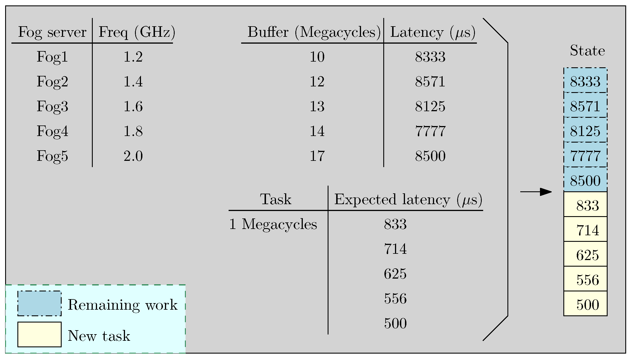
- We propose a reinforcement learning model for the real-time task assignment in fog networks with the objective of minimizing long-term latency. The method for crafting states of the system is novel and is an important contribution to the success of the model.
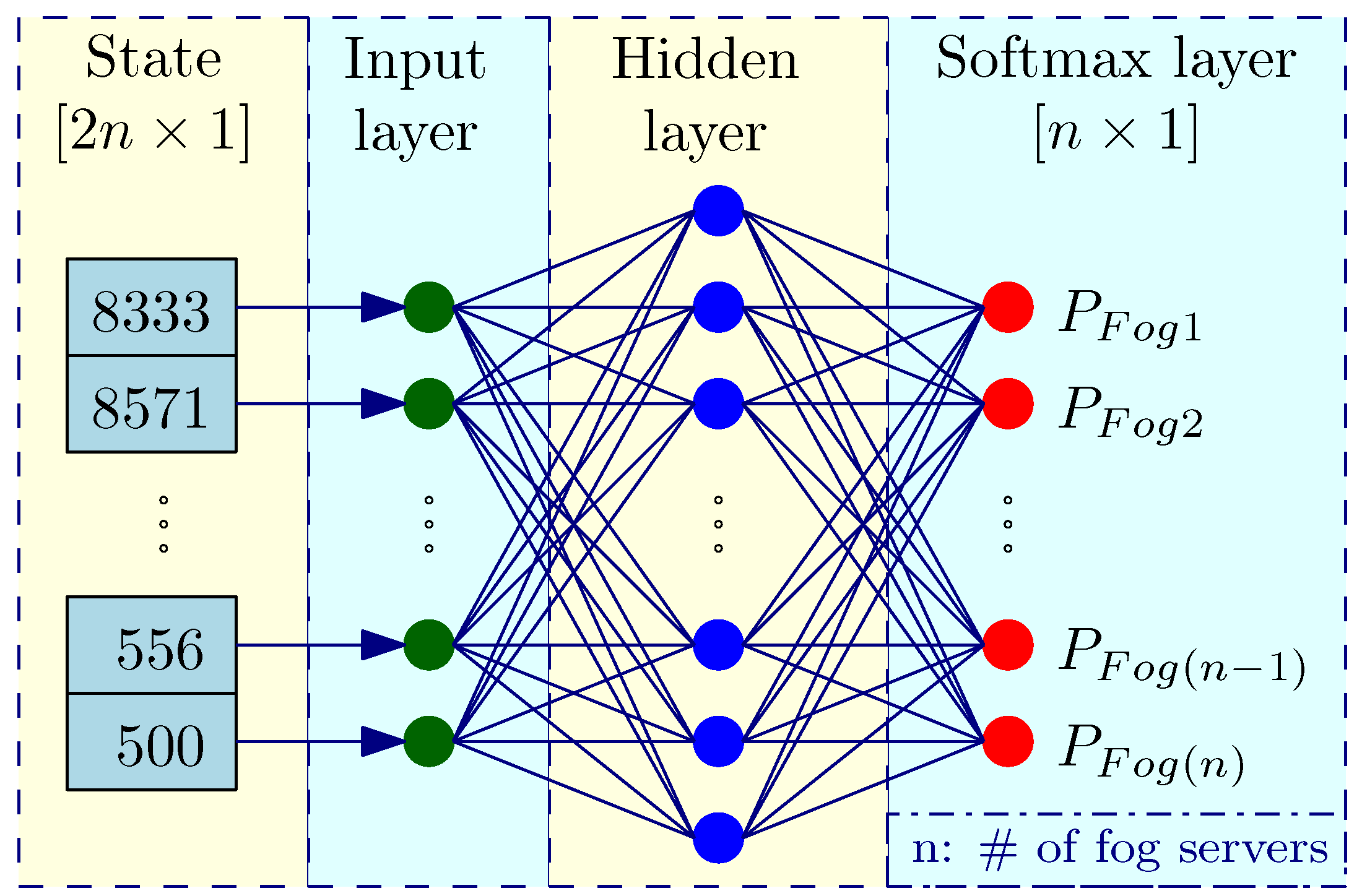
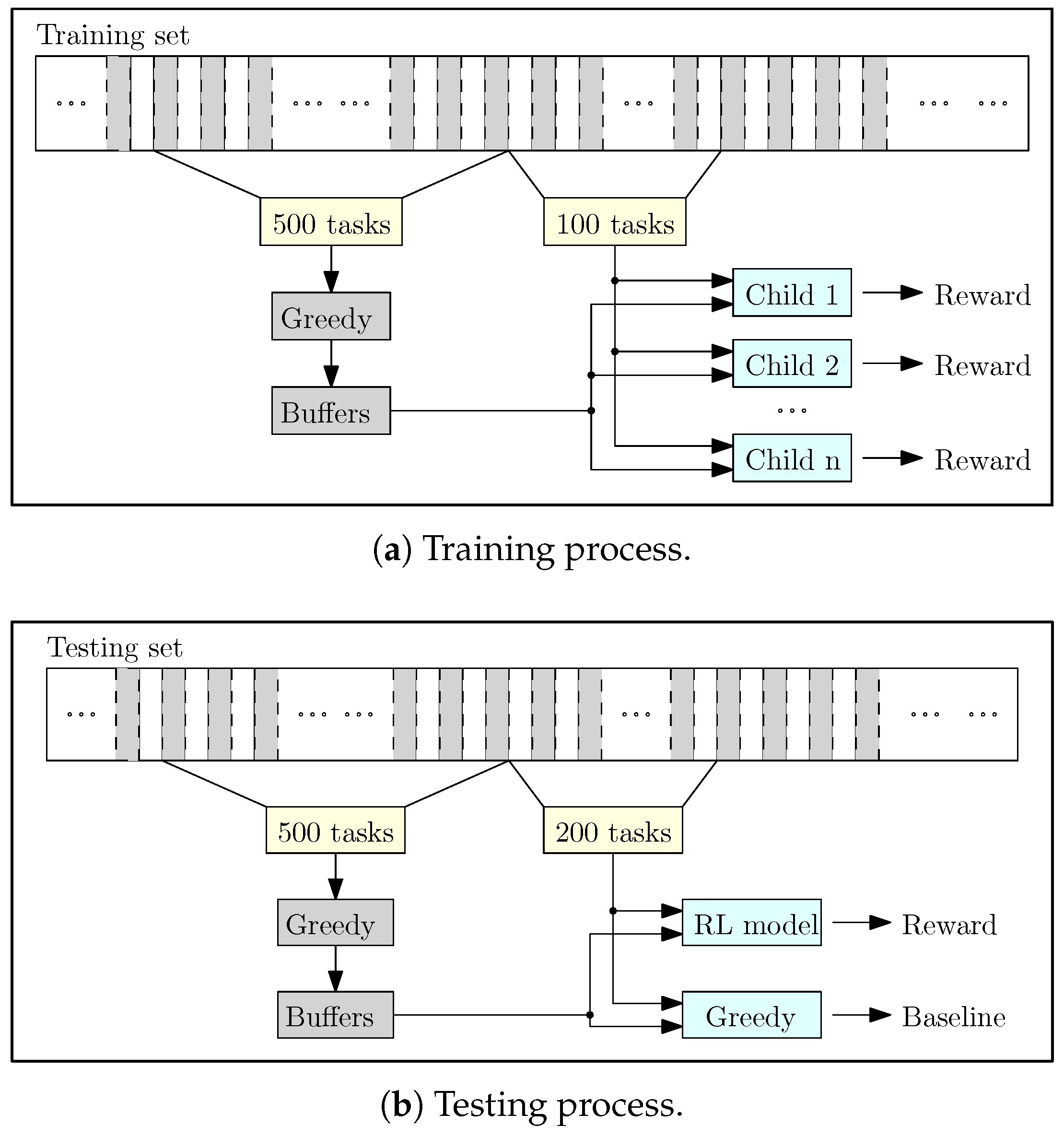
- We propose the evolution strategies as a learning method for the reinforcement learning model for optimizing the server selection function, i.e., the trainable neural network. The algorithm has low computational complexity and simplicity in implementation. Additionally, the algorithm is remarkably parallel due to the independence in evaluation of its children. Therefore, it is suitable for modern computers with parallel CPUs.
- We prove by comprehensive experiments that the proposed model is scalable when the system escalates the number of IoT devices or the number of fog servers. The model attains 15.3% higher reward than the greedy method in a system with 100 IoT devices and five fog servers; and 16.1% with 200 IoT devices and 10 fog servers.
2. Related Work
3. System Model
3.1. Real-Time Task Assignment Problem
3.2. Reinforcement Learning Model
3.3. Action Selection Function
4. Evolution Strategies
| Algorithm 1 Reinforcement learning with evolution strategies. | |
| 1: Given | |
| 2: Parent NN with weight matrix | |
| 3: number of children m | |
| 4: learning_rate | |
| 5: Start | |
| 6: for iteration in a predefined range do | |
| 7: for h in range m do | |
| 8: Parent NN + random noise | () |
| 9: Evaluate | |
| 10: Calculate | |
| 11: | |
| 12: Parent NN → Parent NN + | |
| 13: Evaluate Parent NN | |
| 14: End | |
| Return the highest performing Parent NN | |
5. Experiments
5.1. Experimental Setup
5.1.1. Data Collection
5.1.2. Fog Server and System Setup
5.2. Experimental Method
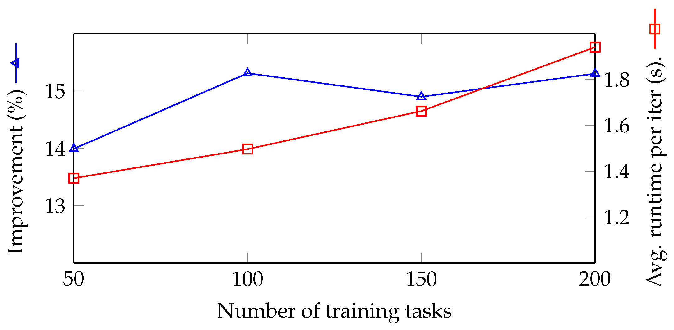
5.3. Results
6. Conclusions
Author Contributions
Funding
Conflicts of Interest
References
- Mouradian, C.; Naboulsi, D.; Yangui, S.; Glitho, R.H.; Morrow, M.J.; Polakos, P.A. A Comprehensive Survey on Fog Computing: State-of-the-art and Research Challenges. IEEE Commun. Surv. Tutor. 2017, 20, 416–464. [Google Scholar] [CrossRef]
- Abbas, N.; Zhang, Y.; Taherkordi, A.; Skeie, T. Mobile edge computing: A survey. IEEE Internet Things J. 2018, 5, 450–465. [Google Scholar] [CrossRef]
- Dao, N.N.; Vu, D.N.; Lee, Y.; Park, M.; Cho, S. MAEC-X: DDoS prevention leveraging multi-access edge computing. In Proceedings of the IEEE International Conference on Information Networking (ICOIN), Chiang Mai, Thailand, 10–12 January 2018; pp. 245–248. [Google Scholar]
- Shih, Y.Y.; Chung, W.H.; Pang, A.C.; Chiu, T.C.; Wei, H.Y. Enabling low-latency applications in fog-radio access networks. IEEE Netw. 2017, 31, 52–58. [Google Scholar] [CrossRef]
- Rahman, G.S.; Peng, M.; Zhang, K.; Chen, S. Radio Resource Allocation for Achieving Ultra-Low Latency in Fog Radio Access Networks. IEEE Access 2018, 6, 17442–17454. [Google Scholar] [CrossRef]
- Dao, N.N.; Lee, Y.; Cho, S.; Kim, E.; Chung, K.S.; Keum, C. Multi-tier multi-access edge computing: The role for the fourth industrial revolution. In Proceedings of the IEEE International Conference on Information and Communication Technology Convergence (ICTC), Jeju, Korea, 18–20 October 2017; pp. 1280–1282. [Google Scholar]
- Peng, M.; Yan, S.; Zhang, K.; Wang, C. Fog-computing-based radio access networks: Issues and challenges. IEEE Netw. 2016, 30, 46–53. [Google Scholar] [CrossRef]
- Vu, D.N.; Dao, N.N.; Jang, Y.; Na, W.; Kwon, Y.B.; Kang, H.; Jung, J.J.; Cho, S. Joint energy and latency optimization for upstream IoT offloading services in fog radio access networks. Trans. Emerg. Telecommun. Technol. 2018, 29, e3497. [Google Scholar] [CrossRef]
- Sutton, R.S.; Barto, A.G. Reinforcement Learning: An Introduction; MIT Press: Cambridge, UK, 1998; Volume 1. [Google Scholar]
- He, Y.; Yu, F.R.; Zhao, N.; Leung, V.C.; Yin, H. Software-defined networks with mobile edge computing and caching for smart cities: A big data deep reinforcement learning approach. IEEE Commun. Mag. 2017, 55, 31–37. [Google Scholar] [CrossRef]
- He, Y.; Zhao, N.; Yin, H. Integrated Networking, Caching, and Computing for Connected Vehicles: A Deep Reinforcement Learning Approach. IEEE Trans. Veh. Technol. 2018, 67, 44–55. [Google Scholar] [CrossRef]
- Michalewicz, Z. Evolution strategies and other methods. In Genetic Algorithms + Data Structures = Evolution Programs; Springer: Berlin/Heidelberg, Germany, 1996; pp. 159–177. [Google Scholar]
- Salimans, T.; Ho, J.; Chen, X.; Sutskever, I. Evolution strategies as a scalable alternative to reinforcement learning. arXiv, 2017; arXiv:1703.03864. [Google Scholar]
- Bishop, C.; Bishop, C.M. Neural Networks for Pattern Recognition; Oxford University Press: Oxford, UK, 1995. [Google Scholar]
- Nasrabadi, N.M. Pattern recognition and machine learning. J. Electron. Imaging 2007, 16, 049901. [Google Scholar]
- Mahmud, R.; Kotagiri, R.; Buyya, R. Fog computing: A taxonomy, survey and future directions. In Internet of Everything; Springer: Berlin/Heidelberg, Germany, 2018; pp. 103–130. [Google Scholar]
- Mukherjee, M.; Shu, L.; Wang, D. Survey of Fog Computing: Fundamental, Network Applications, and Research Challenges. IEEE Commun. Surv. Tutor. 2018, 20, 1826–1857. [Google Scholar] [CrossRef]
- Mach, P.; Becvar, Z. Mobile edge computing: A survey on architecture and computation offloading. IEEE Commun. Surv. Tutor. 2017, 19, 1628–1656. [Google Scholar] [CrossRef]
- Markakis, E.K.; Karras, K.; Sideris, A.; Alexiou, G.; Pallis, E. Computing, Caching, and Communication at the Edge: The Cornerstone for Building a Versatile 5G Ecosystem. IEEE Commun. Mag. 2017, 55, 152–157. [Google Scholar] [CrossRef]
- Kim, S. 5G Network Communication, Caching, and Computing Algorithms Based on the Two-Tier Game Model. ETRI J. 2018, 40, 61–71. [Google Scholar] [CrossRef] [Green Version]
- Paščinski, U.; Trnkoczy, J.; Stankovski, V.; Cigale, M.; Gec, S. QoS-aware orchestration of network intensive software utilities within software defined data centres. J. Grid Comput. 2018, 16, 85–112. [Google Scholar] [CrossRef]
- Hu, Y.; Wang, J.; Zhou, H.; Martin, P.; Taal, A.; de Laat, C.; Zhao, Z. Deadline-aware deployment for time critical applications in clouds. In Proceedings of the European Conference on Parallel Processing, Compostela, Spain, 28 August–1 September 2017; pp. 345–357. [Google Scholar]
- Chamola, V.; Tham, C.K.; Chalapathi, G.S. Latency aware mobile task assignment and load balancing for edge cloudlets. In Proceedings of the IEEE International Conference on Pervasive Computing and Communications Workshops (PerCom Workshops), Kona, HI, USA, 13–17 March 2017; pp. 587–592. [Google Scholar]
- Dao, N.N.; Vu, D.N.; Lee, Y.; Cho, S.; Cho, C.; Kim, H. Pattern-Identified Online Task Scheduling in Multitier Edge Computing for Industrial IoT Services. Mob. Inf. Syst. 2018, 2018, 2101206. [Google Scholar] [CrossRef]
- Ali, M.; Riaz, N.; Ashraf, M.I.; Qaisar, S.; Naeem, M. Joint Cloudlet Selection and Latency Minimization in Fog Networks. IEEE Trans. Ind. Inform. 2018, 99. [Google Scholar] [CrossRef]
- Dao, N.N.; Lee, J.; Vu, D.N.; Paek, J.; Kim, J.; Cho, S.; Chung, K.S.; Keum, C. Adaptive resource balancing for serviceability maximization in fog radio access networks. IEEE Access 2017, 5, 14548–14559. [Google Scholar] [CrossRef]
- Witten, I.H.; Frank, E.; Hall, M.A.; Pal, C.J. Data Mining: Practical Machine Learning Tools and Techniques; Morgan Kaufmann: Burlington, MA, USA, 2016. [Google Scholar]
- Mnih, V.; Kavukcuoglu, K.; Silver, D.; Rusu, A.A.; Veness, J.; Bellemare, M.G.; Graves, A.; Riedmiller, M.; Fidjeland, A.K.; Ostrovski, G.; et al. Human-level control through deep reinforcement learning. Nature 2015, 518, 529. [Google Scholar] [CrossRef] [PubMed]
- Van Hasselt, H.; Guez, A.; Silver, D. Deep Reinforcement Learning with Double Q-Learning. In Proceedings of the AAAI, Phoenix, AZ, USA, 12–17 February 2016; Volume 16, pp. 2094–2100. [Google Scholar]
- Wang, Z.; Schaul, T.; Hessel, M.; Hasselt, H.; Lanctot, M.; Freitas, N. Dueling Network Architectures for Deep Reinforcement Learning. In Proceedings of the International Conference on Machine Learning, New York, NY, USA, 19–24 June 2016; pp. 1995–2003. [Google Scholar]
- Hornik, K.; Stinchcombe, M.; White, H. Multilayer feedforward networks are universal approximators. Neural Netw. 1989, 2, 359–366. [Google Scholar] [CrossRef]
- Silver, D.; Huang, A.; Maddison, C.J.; Guez, A.; Sifre, L.; Van Den Driessche, G.; Schrittwieser, J.; Antonoglou, I.; Panneershelvam, V.; Lanctot, M.; et al. Mastering the game of Go with deep neural networks and tree search. Nature 2016, 529, 484–489. [Google Scholar] [CrossRef] [PubMed]
- LeCun, Y.; Bengio, Y.; Hinton, G. Deep learning. Nature 2015, 521, 436. [Google Scholar] [CrossRef] [PubMed]
- Goodfellow, I.; Bengio, Y.; Courville, A.; Bengio, Y. Deep Learning; MIT Press: Cambridge, MA, USA, 2016; Volume 1. [Google Scholar]
- Such, F.P.; Madhavan, V.; Conti, E.; Lehman, J.; Stanley, K.O.; Clune, J. Deep Neuroevolution: Genetic Algorithms Are a Competitive Alternative for Training Deep Neural Networks for Reinforcement Learning. arXiv, 2017; arXiv:1712.06567. [Google Scholar]
- Mnih, V.; Kavukcuoglu, K.; Silver, D.; Graves, A.; Antonoglou, I.; Wierstra, D.; Riedmiller, M. Playing atari with deep reinforcement learning. arXiv, 2013; arXiv:1312.5602. [Google Scholar]
- Schwarzkopf, M.; Konwinski, A.; Abd-El-Malek, M.; Wilkes, J. Omega: Flexible, scalable schedulers for large compute clusters. In Proceedings of the 8th ACM European Conference on Computer Systems, Prague, Czech Republic, 14–17 April 2013; pp. 351–364. [Google Scholar]
- Hindman, B.; Konwinski, A.; Zaharia, M.; Ghodsi, A.; Joseph, A.D.; Katz, R.H.; Shenker, S.; Stoica, I. Mesos: A Platform for Fine-Grained Resource Sharing in the Data Center. In Proceedings of the 8th USENIX Conference on Networked Systems Design and Implementation, Boston, MA, USA, 30 March–1 April 2011; Volume 11, p. 22. [Google Scholar]
- Bernstein, D. Containers and cloud: From lxc to docker to kubernetes. IEEE Cloud Comput. 2014, 1, 81–84. [Google Scholar] [CrossRef]
- Vecchiola, C.; Chu, X.; Buyya, R. Aneka: A software platform for .NET-based cloud computing. High Speed Large Scale Sci. Comput. 2009, 18, 267–295. [Google Scholar]


| Term | Explanation | Unit |
|---|---|---|
| Fog(n) | n-th fog server | |
| Exp(n) | n-th experiment | |
| Capability (i.e., frequency) of Fog(n) | Number of cycles that Fog(n) can complete per second | Hz |
| Size of a task | Number of bits in a task | bit |
| Complexity of a task | Number of cycles needed to solve a bit of the task | cycles/bit |
| Remaining tasks in a buffer | Tasks in the buffer at a given time | |
| Latency of Fog(n) | Computational latency of Fog(n) for completing the remaining tasks in its buffer | second |
| System latency | Maximum latency among all fog servers | second |
| (a) Greedy methods. | |||||||
| Time | Task | Size (Mbits) | Complexity (Cycles/bit) | Expected latency (Fog1-Fog2) | Fog1 latency | Fog2 latency | System latency |
| 0 ms | 0 | 0 | 0 | ||||
| Task1 | 1 | 10 | 5 ms–10 ms | 5 ms | 0 | 5 ms | |
| 2 ms | 3 ms | 0 | |||||
| Task2 | 1 | 7 | 3.5 ms–7 ms | 6.5 ms | 0 | ||
| Task3 | 1 | 8 | 4 ms–8 ms | 6.5 ms | 8 ms | 8 ms | |
| (b) Long-term latency optimization. | |||||||
| Time | Task | Size (Mbits) | Complexity (Cycles/bit) | Expected latency (Fog1-Fog2) | Fog1 latency | Fog2 latency | System latency |
| 0 ms | 0 | 0 | 0 | ||||
| Task1 | 1 | 10 | 5 ms–10 ms | 5 ms | 0 | 5 ms | |
| 2 ms | 3 ms | 0 | |||||
| Task2 | 1 | 7 | 3.5 ms–7 ms | 3 ms | 7 ms | ||
| Task3 | 1 | 8 | 4 ms–8 ms | 7 ms | 7 ms | 7 ms | |
| Parameter | Experiment | Initial |
|---|---|---|
| # of Fog servers | 5, 10 | 5 |
| # of IoT nodes | 100, 200 | 100 |
| # of training tasks | 50, 100, 150, 200 | 100 |
| Learning rate | 0.002 | Fixed |
| # of children | 5, 10, 15, 20 | 10 |
| Deviation of children | 0.2 | Fixed |
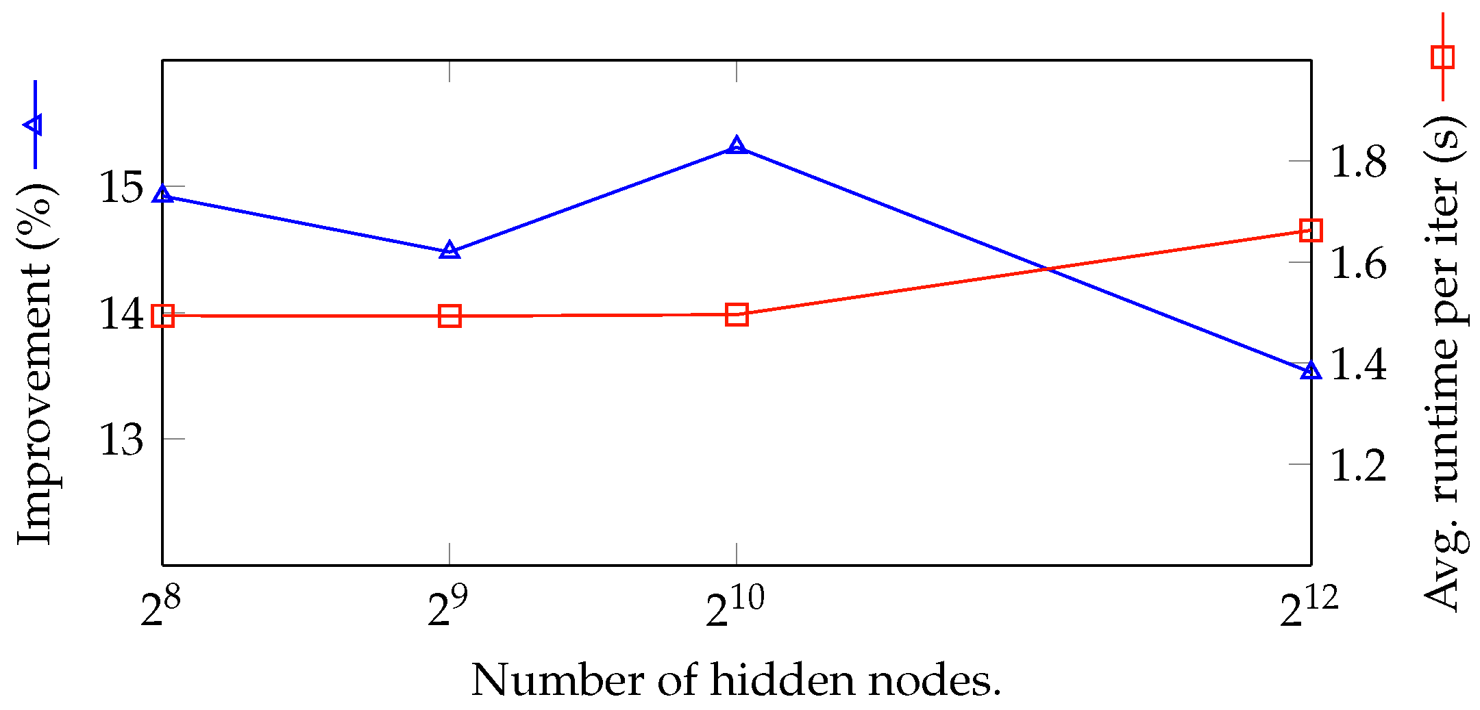
| # of hidden nodes in NN | 256, 512, 1024, 4096 | 1024 |
| Experiment | # of Servers | # of IoT Devices | # of Training Tasks | # of Children | # of Hidden Nodes in NN | Our Model | Greedy Method | Improvement (%) | Average Runtime Per Iter (s) |
|---|---|---|---|---|---|---|---|---|---|
| 1 | 5 | 100 | 100 | 10 | 1024 | 357.305 | 309.867 | 15.309 | 1.496 |
| 2 | 10 | 200 | 100 | 10 | 1024 | 346.509 | 298.455 | 16.101 | 1.667 |
| 3 | 5 | 100 | 50 | 10 | 1024 | 353.208 | 309.867 | 13.989 | 1.369 |
| 1 | 5 | 100 | 100 | 10 | 1024 | 357.305 | 309.867 | 15.309 | 1.496 |
| 4 | 5 | 100 | 150 | 10 | 1024 | 356.030 | 309.867 | 14.898 | 1.662 |
| 5 | 5 | 100 | 200 | 10 | 1024 | 357.2822 | 309.867 | 15.302 | 1.941 |
| 6 | 5 | 100 | 100 | 5 | 1024 | 352.169 | 309.867 | 13.652 | 1.345 |
| 1 | 5 | 100 | 100 | 10 | 1024 | 357.305 | 309.867 | 15.309 | 1.496 |
| 7 | 5 | 100 | 100 | 15 | 1024 | 359.002 | 309.867 | 15.857 | 1.659 |
| 8 | 5 | 100 | 100 | 20 | 1024 | 357.031 | 309.867 | 15.221 | 1.838 |
| 9 | 5 | 100 | 100 | 10 | 256 | 356.107 | 309.867 | 14.923 | 1.494 |
| 10 | 5 | 100 | 100 | 10 | 512 | 354.732 | 309.867 | 14.479 | 1.493 |
| 1 | 5 | 100 | 100 | 10 | 1024 | 357.305 | 309.867 | 15.309 | 1.496 |
| 11 | 5 | 100 | 100 | 10 | 4096 | 351.781 | 309.867 | 13.526 | 1.663 |
© 2018 by the authors. Licensee MDPI, Basel, Switzerland. This article is an open access article distributed under the terms and conditions of the Creative Commons Attribution (CC BY) license (http://creativecommons.org/licenses/by/4.0/).
Share and Cite
Mai, L.; Dao, N.-N.; Park, M. Real-Time Task Assignment Approach Leveraging Reinforcement Learning with Evolution Strategies for Long-Term Latency Minimization in Fog Computing. Sensors 2018, 18, 2830. https://doi.org/10.3390/s18092830
Mai L, Dao N-N, Park M. Real-Time Task Assignment Approach Leveraging Reinforcement Learning with Evolution Strategies for Long-Term Latency Minimization in Fog Computing. Sensors. 2018; 18(9):2830. https://doi.org/10.3390/s18092830
Chicago/Turabian StyleMai, Long, Nhu-Ngoc Dao, and Minho Park. 2018. "Real-Time Task Assignment Approach Leveraging Reinforcement Learning with Evolution Strategies for Long-Term Latency Minimization in Fog Computing" Sensors 18, no. 9: 2830. https://doi.org/10.3390/s18092830