Evaluation of Water Indices for Surface Water Extraction in a Landsat 8 Scene of Nepal


Abstract
:1. Introduction
2. Materials and Methods
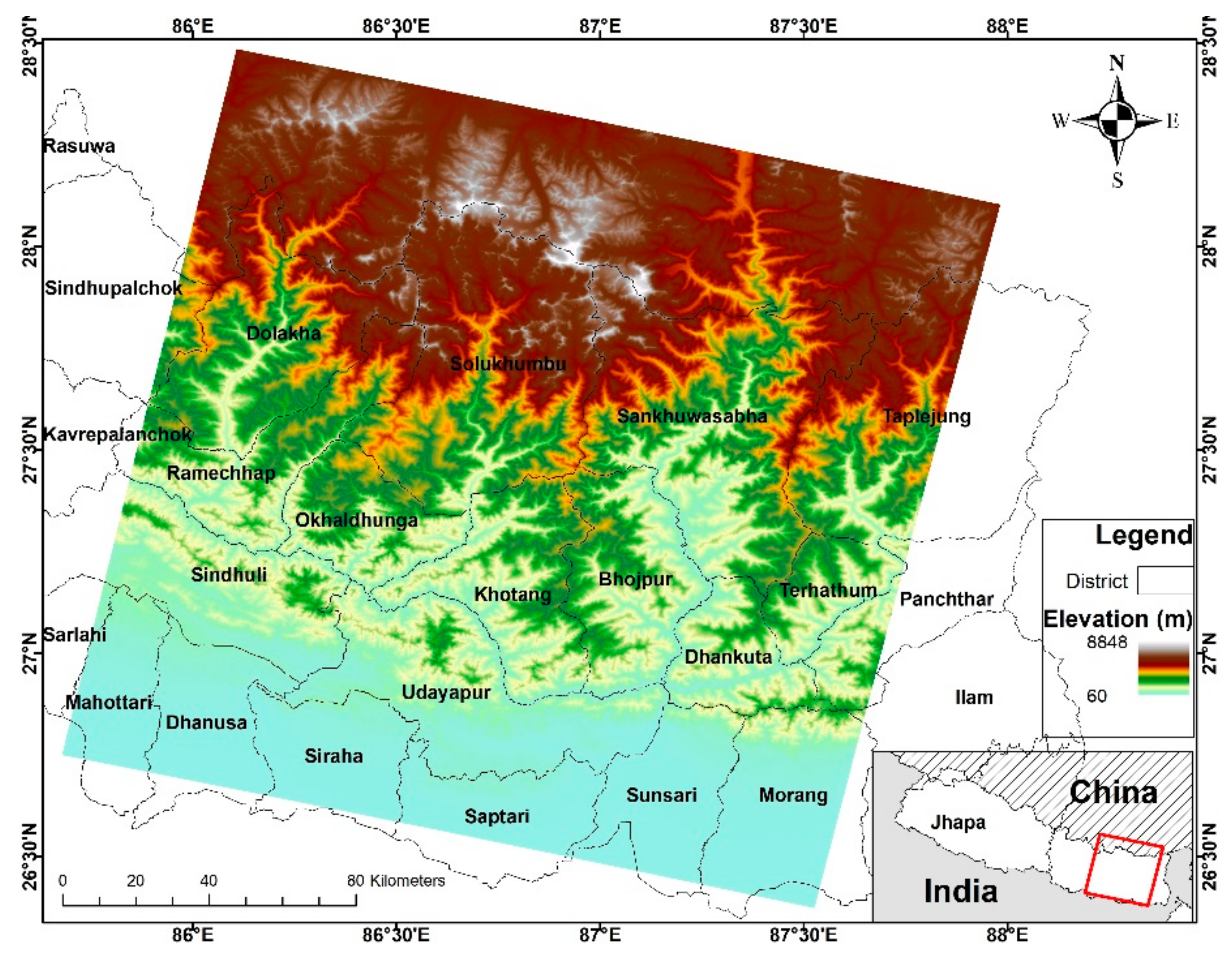
2.1. Test Area
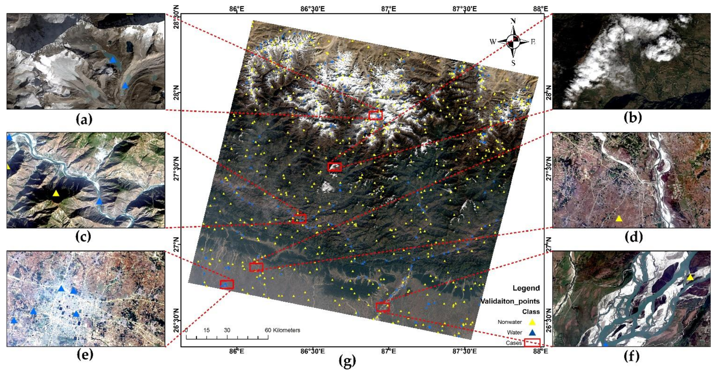
2.2. Data
2.3. Water Indices for Surface Water Extraction
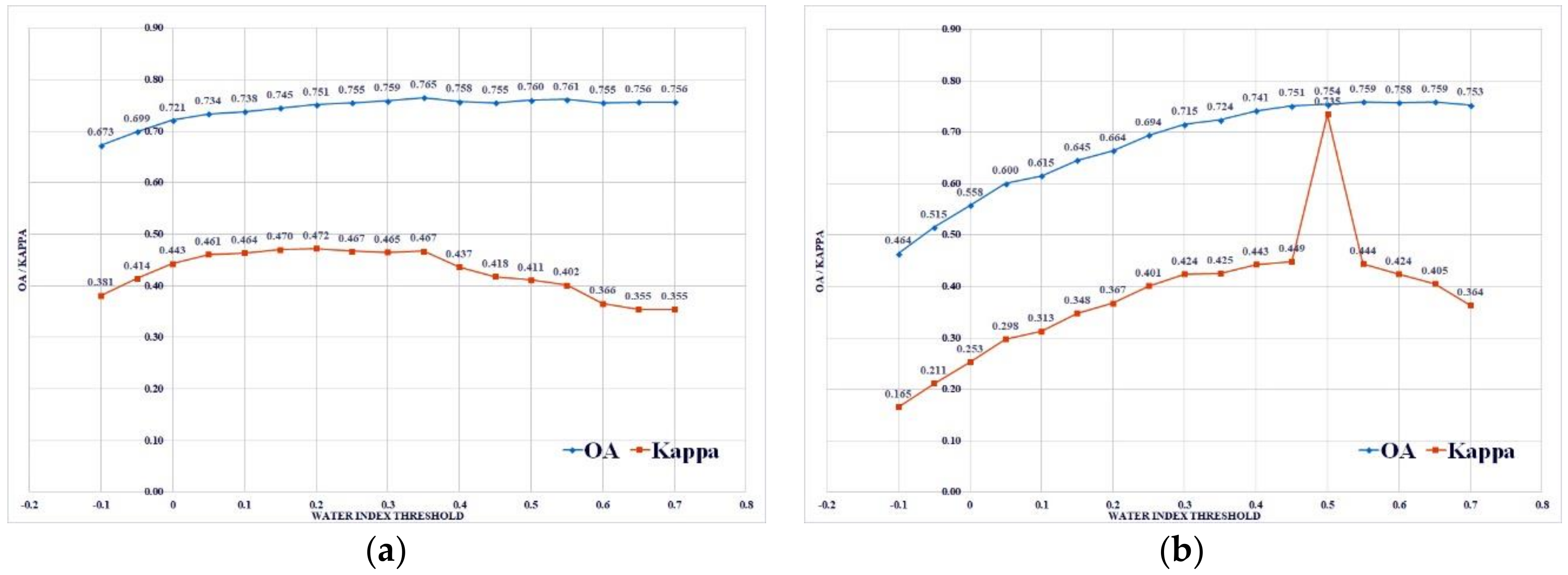
2.4. Accuracy Assessment
- True positive (TP): The number of correctly extracted water pixels;
- False negative (FN): The number of undetected water pixels;
- False positive (FP): The number of incorrectly extracted water pixels; and
- True negative (TN): The number of correctly rejected non-water pixels.
3. Results and Discussion
4. Conclusions
- (a)
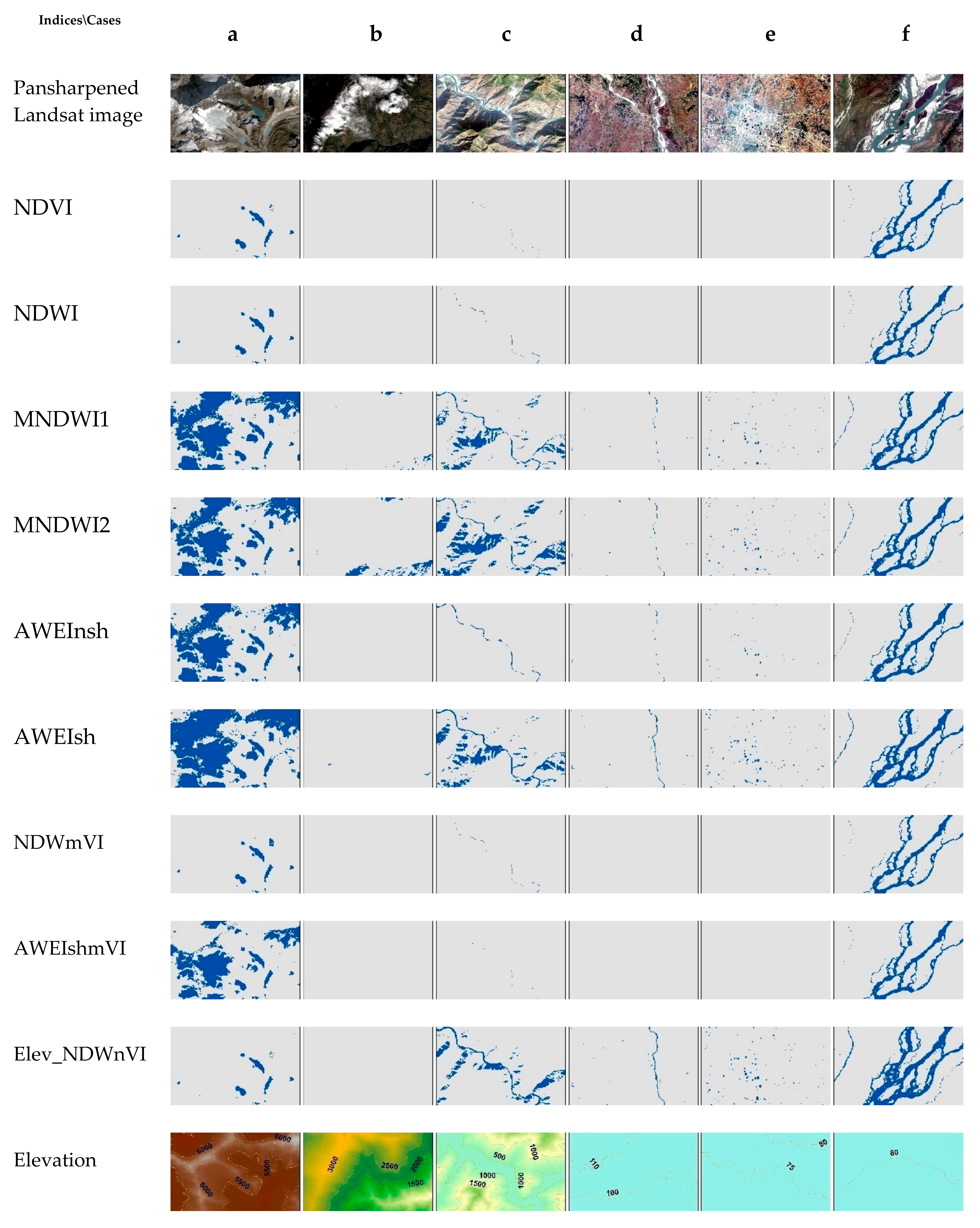
- The standard threshold of all the water indices was able to extract most of the surface water pixels, i.e., high PA, but with many misclassified non-water pixels, i.e., low UA. Based on visual and quantitative evaluations, the standard threshold is not useful in deriving a surface water map in scene with diverse characteristics.
- (b)
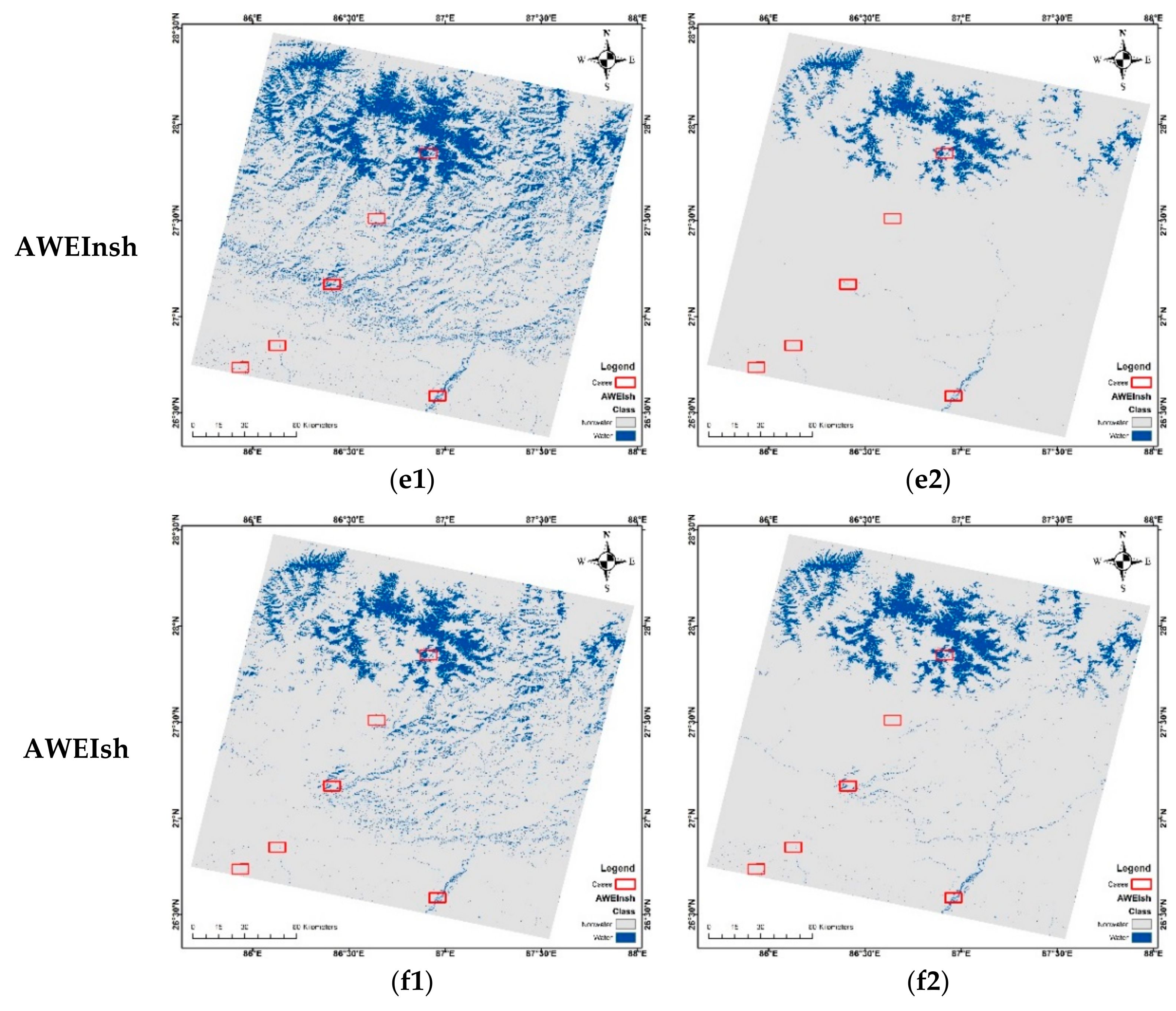
- The optimum threshold improves the detection ability in most of the cases with higher OA, but lower kappa. With an optimum threshold, NDVI and NDWI were good at detecting pure pixels and rejecting the rest, whereas MNDWI and AWEI were able to detect mixed pixels of small ponds and rivers, but unable to reject snow cover and shadow in the Himalayas.
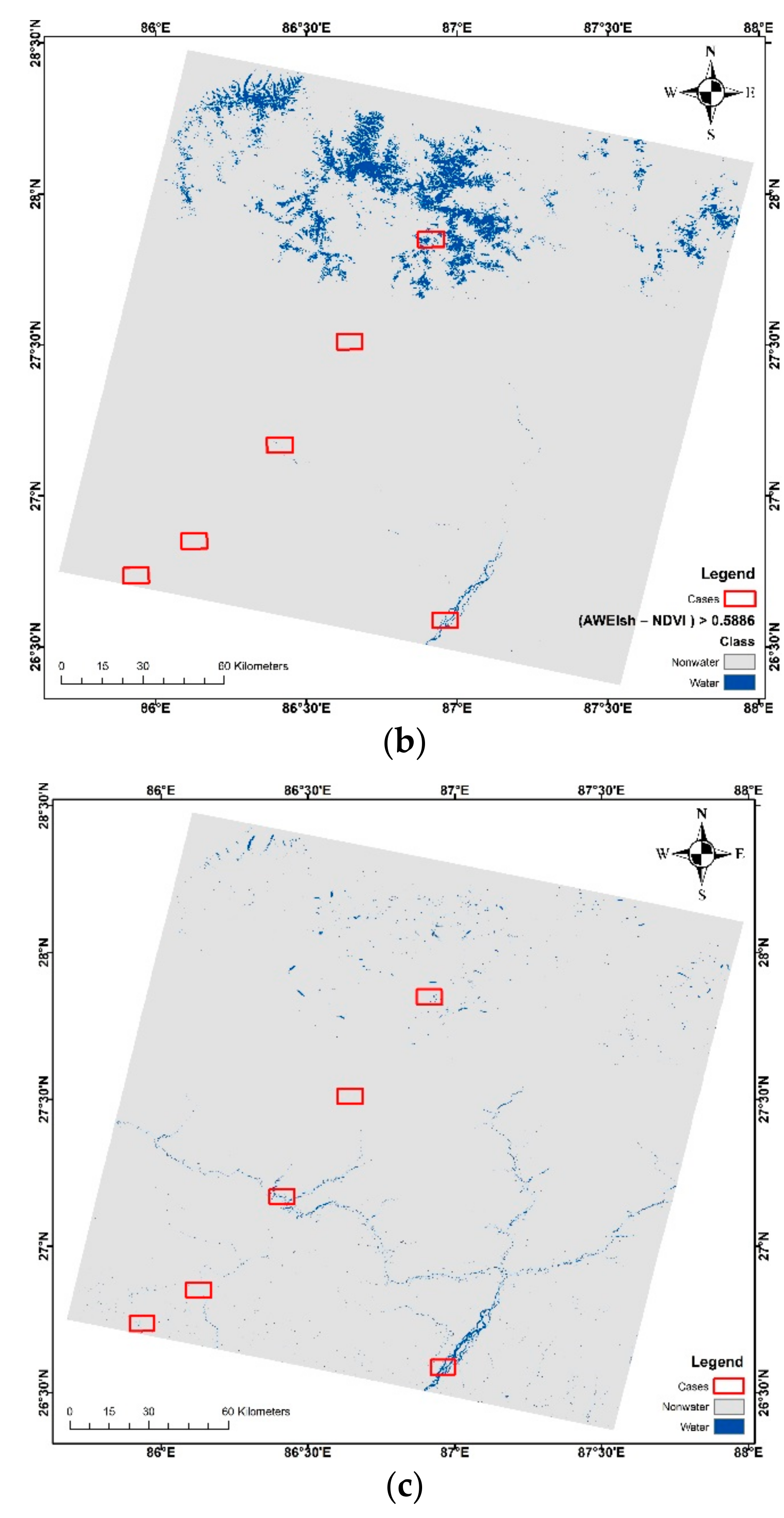
- (c)
- The combined approach for NDWI and AWEIsh with NDVI did not improve the detection ability in the scene.
- (d)
- Segmentation of the scene with elevation showed that NDVI and NDWI can be used for accurate surface water detection for different elevation range and water types. The proposed elevation above and below 665 m used NDVI and NDWI for the surface water detection, respectively. The OA for the proposed method was 0.9638 and the kappa was 0.8979. However, it was susceptible to shadows.
Author Contributions
Funding
Acknowledgments
Conflicts of Interest
References
- Vorosmarty, C.J.; Green, P.; Salisbury, J.; Lammers, R.B. Global water resources: Vulnerability from climate change and population growth. Science 2000, 289, 284–288. [Google Scholar] [CrossRef] [PubMed]
- Pekel, J.; Cottam, A.; Gorelick, N.; Belward, A.S. High-resolution mapping of global surface water and its long-term changes. Nature 2016, 540, 418–422. [Google Scholar] [CrossRef] [PubMed]
- Melesse, A.M.; Weng, Q.; Thenkabail, P.S.; Senay, G.B. Remote sensing sensors and applications in environmental resources mapping and modelling. Sensors 2007, 7, 3209–3241. [Google Scholar] [CrossRef] [PubMed]
- Lee, J.K.; Acharya, T.D.; Lee, D.H. Exploring land cover classification accuracy of Landsat 8 image using spectral index layer stacking in hilly region of South Korea. Sens. Mater. 2018, 30, 1–15. [Google Scholar]
- Acharya, T.D.; Lee, D.H.; Yang, I.T.; Lee, J.K. Identification of water bodies in a Landsat 8 OLI image using a J48 decision tree. Sensors 2016, 16, 1075. [Google Scholar] [CrossRef] [PubMed]
- Karpatne, A.; Khandelwal, A.; Chen, X.; Mithal, V.; Faghmous, J.; Kumar, V. Global monitoring of inland water dynamics: State-of-the-art, challenges, and opportunities. In Computational Sustainability; Lässig, J., Kersting, K., Morik, K., Eds.; Springer International Publishing: Cham, Switzerland, 2016; pp. 121–147. [Google Scholar]
- Tulbure, M.G.; Broich, M. Spatiotemporal dynamic of surface water bodies using Landsat time-series data from 1999 to 2011. ISPRS J. Photogramm. Remote Sens. 2013, 79, 44–52. [Google Scholar] [CrossRef]
- Nath, R.K.; Deb, S.K. Water-body area extraction from high resolution satellite images—An introduction, review, and comparison. Int. J. Image Process. 2010, 3, 353–372. [Google Scholar]
- Sivanpillai, R.; Miller, S.N. Improvements in mapping water bodies using ASTER data. Ecol. Inf. 2010, 5, 73–78. [Google Scholar] [CrossRef]
- Sethre, P.R.; Rundquist, B.C.; Todhunter, P.E. Remote detection of Prairie Pothole Ponds in the Devils Lake Basin, North Dakota. GISci. Remote Sens. 2005, 42, 277–296. [Google Scholar] [CrossRef]
- Klein, I.; Dietz, A.J.; Gessner, U.; Galayeva, A.; Myrzakhmetov, A.; Kuenzer, C. Evaluation of seasonal water body extents in Central Asia over the past 27 years derived from medium-resolution remote sensing data. Int. J. Appl. Earth Obs. Geoinf 2014, 26, 335–349. [Google Scholar] [CrossRef]
- Frazier, P.S.; Page, K.J. Water body detection and delineation with Landsat TM data. Photogramm. Eng. Remote Sens. 2000, 66, 1461–1468. [Google Scholar]
- Work, E.A., Jr.; Gilmer, D.S. Utilization of satellite data for inventorying prairie ponds and lakes. Photogramm. Eng. Remote Sens. 1976, 42, 685–694. [Google Scholar]
- Malahlela, O.E. Inland waterbody mapping: Towards improving discrimination and extraction of inland surface water features. Int. J. Remote Sens. 2016, 37, 4574–4589. [Google Scholar] [CrossRef]
- Feyisa, G.L.; Meilby, H.; Fensholt, R.; Proud, S.R. Automated water extraction index: A new technique for surface water mapping using Landsat imagery. Remote Sens. Environ. 2014, 140, 23–35. [Google Scholar] [CrossRef]
- Ji, L.; Zhang, L.; Wylie, B. Analysis of Dynamic thresholds for the normalized difference water index. Photogramm. Eng. Remote Sens. 2009, 75, 1307–1317. [Google Scholar] [CrossRef]
- Xu, H. Modification of normalised difference water index (NDWI) to enhance open water features in remotely sensed imagery. Int. J. Remote Sens. 2006, 27, 3025–3033. [Google Scholar] [CrossRef]
- Rogers, A.S.; Kearney, M.S. Reducing signature variability in unmixing coastal marsh Thematic Mapper scenes using spectral indices. Int. J. Remote Sens. 2004, 25, 2317–2335. [Google Scholar] [CrossRef]
- McFeeters, S.K. The use of the Normalized Difference Water Index (NDWI) in the delineation of open water features. Int. J. Remote Sens. 1996, 17, 1425–1432. [Google Scholar] [CrossRef]
- Wang, X.; Liu, Y.; Ling, F.; Liu, Y.; Fang, F. Spatio-temporal change detection of Ningbo Coastline using Landsat Time-Series images during 1976–2015. ISPRS Int. J. Geo-Inf. 2017, 6, 68. [Google Scholar] [CrossRef]
- Acharya, T.D.; Yang, I.T.; Subedi, A.; Lee, D.H. Change detection of Lakes in Pokhara, Nepal using Landsat data. Proceedings 2017, 1, 17. [Google Scholar] [CrossRef]
- Ryu, J.; Won, J.; Min, K.D. Waterline extraction from Landsat TM data in a tidal flat: A case study in Gomso Bay, Korea. Remote Sens. Environ. 2002, 83, 442–456. [Google Scholar] [CrossRef]
- Fisher, A.; Danaher, T. A water index for SPOT5 HRG satellite imagery, New South Wales, Australia, determined by linear discriminant analysis. Remote Sens. 2013, 5, 5907. [Google Scholar] [CrossRef]
- Shen, L.; Li, C. Water body extraction from Landsat ETM+ imagery using adaboost algorithm. In Proceedings of the 18th International Conference on Geoinformatics, Beijing, China, 18–20 June 2010; IEEE: Beijing, China; pp. 1–4. [Google Scholar]
- Xiao, X.; Boles, S.; Frolking, S.; Salas, W.; Moore, B.; Li, C.; He, L.; Zhao, R. Observation of flooding and rice transplanting of paddy rice fields at the site to landscape scales in China using VEGETATION sensor data. Int. J. Remote Sens. 2002, 23, 3009–3022. [Google Scholar] [CrossRef]
- Rokni, K.; Ahmad, A.; Selamat, A.; Hazini, S. Water feature extraction and change detection using multitemporal Landsat imagery. Remote Sens. 2014, 6, 4173–4189. [Google Scholar] [CrossRef]
- Acharya, T.D.; Subedi, A.; Yang, I.T.; Lee, D.H. Combining water indices for water and background threshold in Landsat image. Proceedings 2018, 2, 143. [Google Scholar] [CrossRef]
- Acharya, T.D.; Yang, I.T.; Lee, D.H. Surface Water Area Delineation in Landsat OLI Image using Reflectance and SRTM DEM derivatives. In Proceedings of the 2016 Conference on Geo-Spatial Information, Gunsan, Korea, 6–7 October 2016; The Korean Society for Geospatial Information Science: Gunsan, Korea; pp. 233–234. [Google Scholar]
- Lu, S.; Wu, B.; Yan, N.; Wang, H. Water body mapping method with HJ-1A/B satellite imagery. Int. J. Appl. Earth Obs. Geoinf. 2011, 13, 428–434. [Google Scholar] [CrossRef]
- Menarguez, M. Global Water Body Mapping from 1984 to 2015 Using Global High Resolution Multispectral Satellite Imagery; University of Oklahoma: Norman, OK, USA, 2015. [Google Scholar]
- Jiang, H.; Feng, M.; Zhu, Y.; Lu, N.; Huang, J.; Xiao, T. An automated method for extracting rivers and lakes from Landsat imagery. Remote Sens. 2014, 6, 5067–5089. [Google Scholar] [CrossRef]
- Huang, C.; Chen, Y.; Zhang, S.; Wu, J. Detecting, extracting, and monitoring surface water from space using optical sensors: A review. Rev. Geophys. 2018, 56, 333–360. [Google Scholar] [CrossRef]
- Zhou, Y.; Dong, J.; Xiao, X.; Xiao, T.; Yang, Z.; Zhao, G.; Zou, Z.; Qin, Y. Open surface water mapping algorithms: A comparison of water-related spectral indices and sensors. Water 2017, 9, 256. [Google Scholar] [CrossRef]
- Taravat, A.; Rajaei, M.; Emadodin, I.; Hasheminejad, H.; Mousavian, R.; Biniyaz, E. A spaceborne multisensory, multitemporal approach to monitor water level and storage variations of lakes. Water 2016, 8, 478. [Google Scholar] [CrossRef]
- Landsat 8. Available online: http://landsat.usgs.gov/landsat8.php (accessed on 31 July 2017).
- Farr, T.G.; Rosen, P.A.; Caro, E.; Crippen, R.; Duren, R.; Hensley, S.; Kobrick, M.; Paller, M.; Rodriguez, E.; Roth, L.; et al. The shuttle radar topography mission. Rev. Geophys. 2007, 45, 1–33. [Google Scholar] [CrossRef]
- Acharya, T.D.; Yang, I.T.; Lee, D.H. Comparative analysis of digital elevation models between aw3d30, srtm30 and airborne lidar: A case of Chuncheon, South Korea. J. Korean Soc. Surv. Geodesy Photogramm. Cartogr. 2018, 36, 17–24. [Google Scholar]
- Rouse, J.W.; Haas, R.H.; Schell, J.A.; Deering, D.W. Monitoring vegetation systems in the Great Plains with ERTS (Earth Resources Technology Satellite). In Proceedings of the Third Earth Resources Technology Satellite Symposium, Greenbelt, ON, Canada, 10–14 December 1973; pp. 309–317. [Google Scholar]
- McHugh, M.L. Interrater reliability: The kappa statistic. Biochem. Med. 2012, 22, 276–282. [Google Scholar] [CrossRef]
- Yang, X.; Chen, L. Evaluation of automated urban surface water extraction from Sentinel-2A imagery using different water indices. J. Appl. Remote Sens. 2017, 11, 026016. [Google Scholar] [CrossRef]
- Xie, H.; Luo, X.; Xu, X.; Pan, H.; Tong, X. Evaluation of Landsat 8 OLI imagery for unsupervised inland water extraction. Int. J. Remote Sens. 2016, 37, 1826–1844. [Google Scholar] [CrossRef]


| Satellite/Sensor | Band | Wavelength (µm) | Name | Resolution (m) |
|---|---|---|---|---|
| Landsat 8/OLI | 1 | 0.435–0.451 | Coastal Aerosol (CA) | 30 |
| 2 | 0.452–0.512 | Blue | ||
| 3 | 0.533–0.590 | Green | ||
| 4 | 0.636–0.673 | Red | ||
| 5 | 0.851–0.879 | Near Infrared (NIR) | ||
| 6 | 1.566–1.651 | Shortwave NIR 1 (SWIR1) | ||
| 7 | 2.107–2.294 | Shortwave NIR 2 (SWIR2) | ||
| 9 | 1.363–1.384 | Panchromatic | 15 |
| Multiband Index | Equation | Water Value | Reference |
|---|---|---|---|
| Normalized Difference Vegetation Index | NDVI = (NIR − Red)/(NIR + Red) | Negative | [38] |
| Normalized Difference Water Index | NDWI = (Green − NIR)/(Green + NIR) | Positive | [19] |
| Modified Normalized Difference Water Index | MNDWI1 = (Green − SWIR1)/(Green + SWIR1) MNDWI2 = (Green − SWIR2)/(Green + SWIR2) | Positive | [17] |
| Automated Water Extraction Index | AWEIsh = Blue + 2.5 × Green − 1.5 × (NIR + SWIR1) − 0.25 × SWIR2 AWEInsh = 4 × (Green − SWIR1) − (0.25 × NIR + 2.75 × SWIR1) | Positive | [15] |
| Reference Data | |||
|---|---|---|---|
| Water | Non-Water | ||
| Classified data | Water | TP | FP |
| Non-water | FN | TN | |
| Multiband Index | NDVI | NDWI | MNDWI1 | MNDWI2 | AWEInsh | AWEIsh |
|---|---|---|---|---|---|---|
| Optimum thresholds | −0.2955 | 0.3877 | 0.35 | 0.5 | 0.1897 | 0.1112 |
| Index | Standard Threshold | Optimum Threshold | ||||||
|---|---|---|---|---|---|---|---|---|
| PA | UA | OA | Kappa | PA | UA | OA | Kappa | |
| NDVI | 0.8495 | 0.4907 | 0.76 | 0.4641 | 0.5 | 0.949 | 0.8775 | 0.589 |
| NDWI | 0.9301 | 0.5 | 0.7675 | 0.4988 | 0.5323 | 0.8919 | 0.8762 | 0.5966 |
| MNDWI1 | 0.9785 | 0.4539 | 0.7212 | 0.4432 | 0.7742 | 0.4865 | 0.7575 | 0.4366 |
| MNDWI2 | 0.9946 | 0.3439 | 0.5575 | 0.2529 | 0.8763 | 0.4697 | 0.7412 | 0.443 |
| AWEInsh | 0.8495 | 0.4788 | 0.75 | 0.4484 | 0.6183 | 0.5134 | 0.775 | 0.4115 |
| AWEIsh | 0.9839 | 0.4598 | 0.7275 | 0.4535 | 0.9409 | 0.5287 | 0.7912 | 0.5401 |
| S. No. | Given Abb. | Segmentation | Index | Threshold | PA | UA | OA | Kappa |
|---|---|---|---|---|---|---|---|---|
| 1 | NDWmVI | - | NDWI—NDVI | 0.6638 | 0.5376 | 0.9091 | 0.8800 | 0.6079 |
| 2 | AWEIshmVI | - | AWEIsh—NDVI | 0.5886 | 0.4946 | 0.6093 | 0.8088 | 0.4265 |
| 3 | Elev_NDWnVI | Elevation > 665 m | NDVI | −0.295 | 0.9140 | 0.929 | 0.9638 | 0.8979 |
| Elevation < 665 m | NDWI | −0.05 |
© 2018 by the authors. Licensee MDPI, Basel, Switzerland. This article is an open access article distributed under the terms and conditions of the Creative Commons Attribution (CC BY) license (http://creativecommons.org/licenses/by/4.0/).
Share and Cite
Acharya, T.D.; Subedi, A.; Lee, D.H. Evaluation of Water Indices for Surface Water Extraction in a Landsat 8 Scene of Nepal. Sensors 2018, 18, 2580. https://doi.org/10.3390/s18082580
Acharya TD, Subedi A, Lee DH. Evaluation of Water Indices for Surface Water Extraction in a Landsat 8 Scene of Nepal. Sensors. 2018; 18(8):2580. https://doi.org/10.3390/s18082580
Chicago/Turabian StyleAcharya, Tri Dev, Anoj Subedi, and Dong Ha Lee. 2018. "Evaluation of Water Indices for Surface Water Extraction in a Landsat 8 Scene of Nepal" Sensors 18, no. 8: 2580. https://doi.org/10.3390/s18082580