A Service-Constrained Positioning Strategy for an Autonomous Fleet of Airborne Base Stations


Abstract
:1. Introduction
2. System Overview
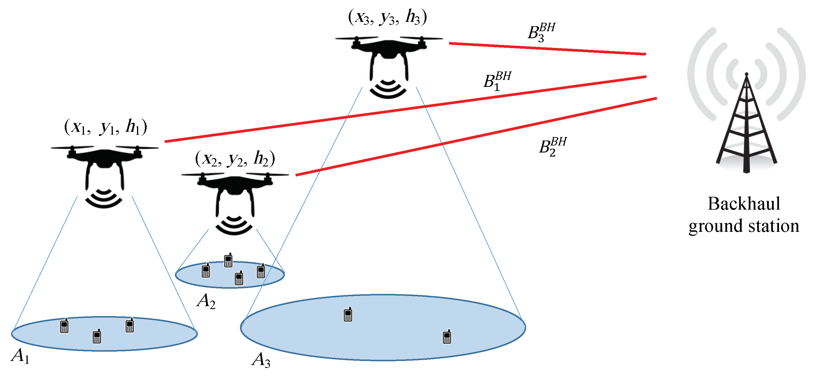
2.1. Scenario
2.2. Channel Model
3. Single Cell User Scheduling
3.1. Round Robin Scheduler
3.2. Equal Rate Scheduler
4. Positioning and Communication for a Fleet of UAVs
4.1. Problem Formulation
4.2. Derivation of the UAV Trajectories
4.2.1. Gradient of the Cost Function
4.2.2. Gradient of the Wireless Backhaul Constraint Functions
| Algorithm 1 Positioning Strategy. | |
| 1: | Start iteration |
| 2: | for do |
| 3: | if then |
| 4: | Add index i to the unfulfilled constraints vector |
| 5: | end if |
| 6: | end for |
| 7: | ifthen |
| 8: | Add the index to |
| 9: | end if |
| 10: | if is empty then |
| 11: | go to 20 |
| 12: | else |
| 13: | Randomly select one constraint of |
| 14: | end if |
| 15: | if selected then |
| 16: | go to 24 |
| 17: | else [the selected index is ] |
| 18: | go to 27 |
| 19: | end if |
| 20: | Calculate for each region using Equation (22) |
| 21: | Identify the region with the lowest |
| 22: | Find the UAVs to be moved |
| 23: | Update the positions of the selected UAVs using Equation (28) and taking into account the restrictions imposed by the maximum feasible velocities. Then, go to 29 |
| 24: | Find the UAVs to be moved |
| 25: | Update the positions of the selected UAVs using Equation (32) and taking into account the restrictions imposed by the maximum feasible velocities |
| 26: | Update using Equation (33) and go to 28 |
| 27: | Subtract a portion from all the bandwidths |
| 28: | Empty |
| 29: | End iteration |
4.3. Practical Implementation Aspects
5. Energy Consumption
5.1. Vertical Flight

5.2. Forward Flight
6. Evaluation and Results
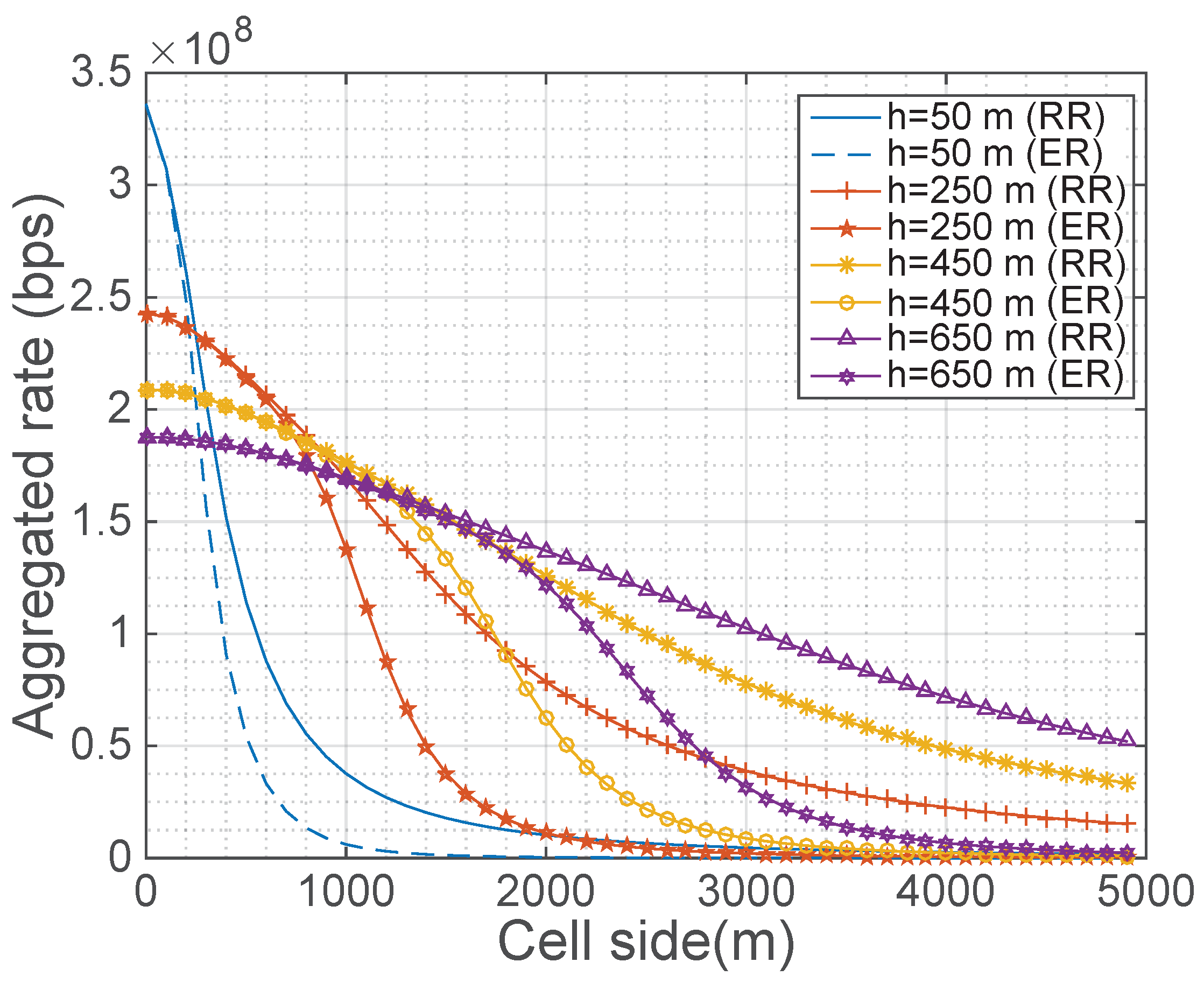
6.1. Scheduling Evaluation
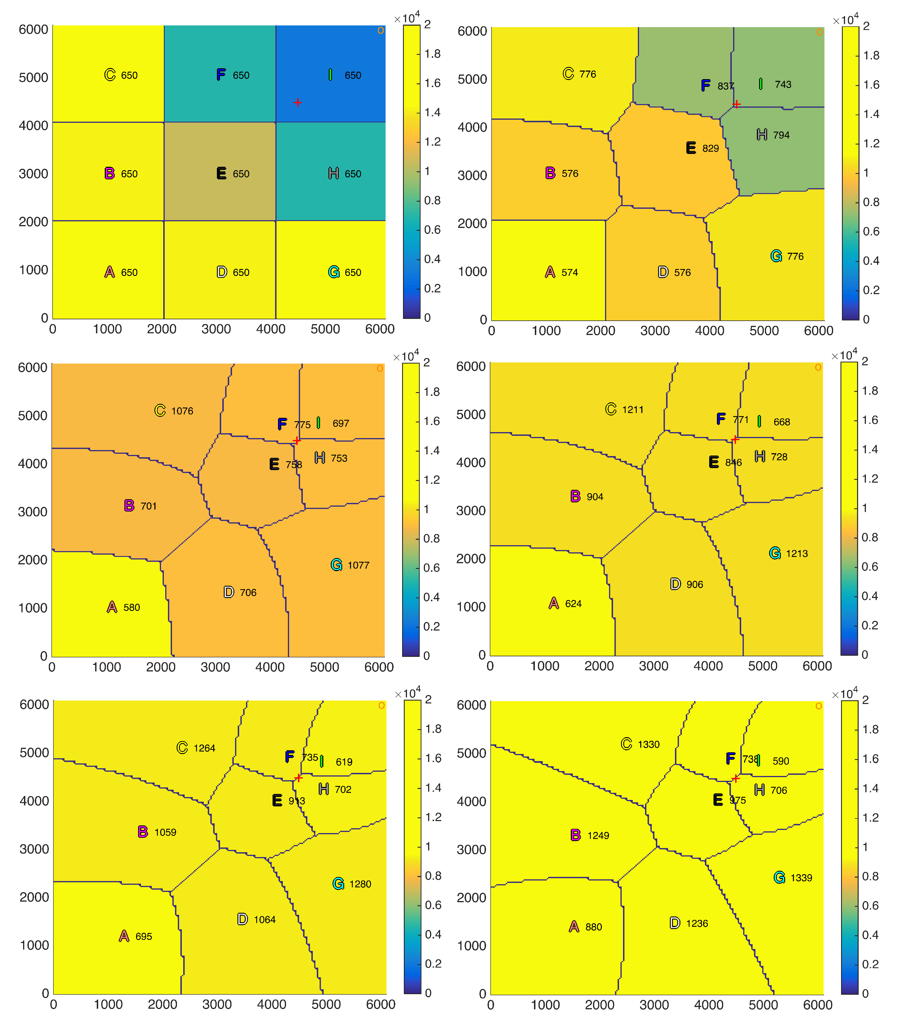
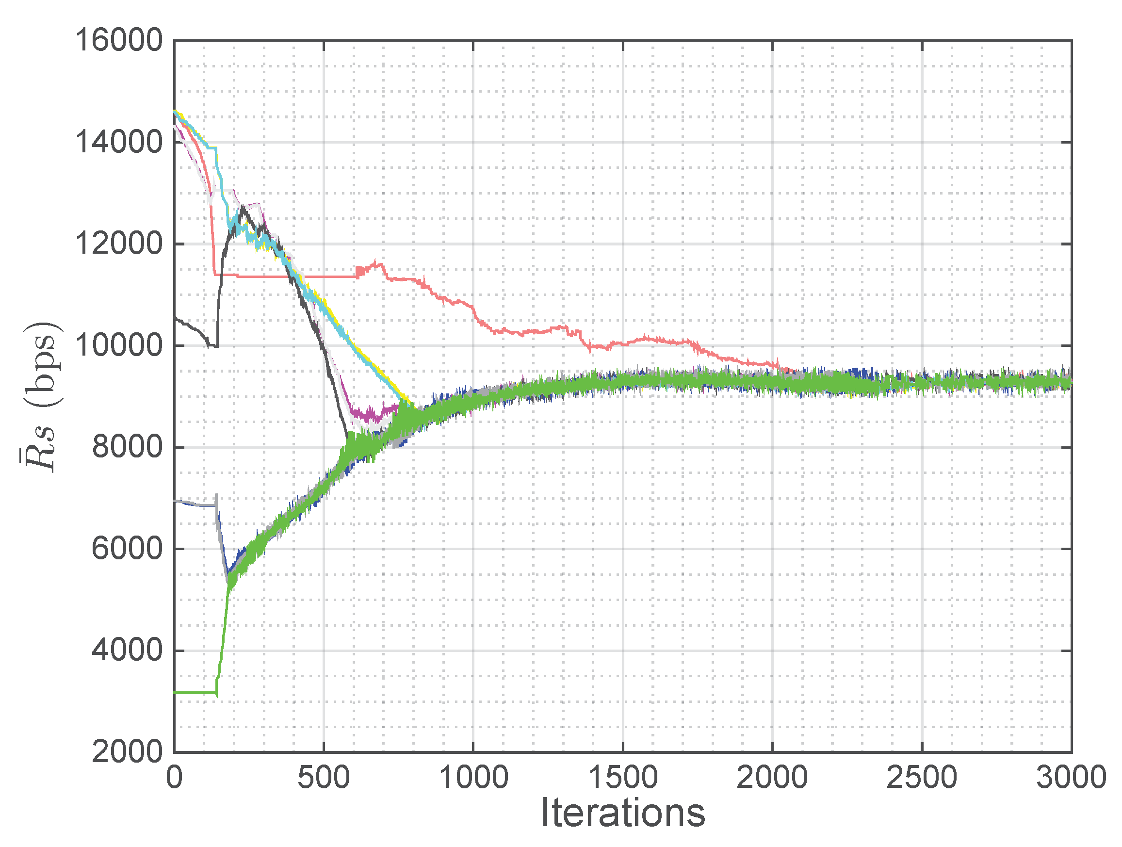
6.2. Positioning Strategy Evaluation
6.3. Comparison to Previous Works
6.3.1. Spiral Algorithm
6.3.2. k-Means Algorithm
6.3.3. Comparison
6.4. Non-Static Scenarios
6.4.1. One UAV Decays
6.4.2. Displacement of the Concentration of Users
6.4.3. Scattering of the Concentration of Users
6.5. Energy Consumption Evaluation
7. Conclusions
Author Contributions
Funding
Conflicts of Interest
References
- Ahmed, N.; Kanhere, S.S.; Jha, S. On the importance of link characterization for aerial wireless sensor networks. IEEE Commun. Mag. 2016, 54, 52–57. [Google Scholar] [CrossRef]
- Feng, Q.; McGeehan, J.; Tameh, E.K.; Nix, A.R. Path loss models for air-to-ground radio channels in urban environments. In Proceedings of the 2006 IEEE 63rd Vehicular Technology Conference (VTC), Melbourne, Australia, 7–10 May 2006; pp. 2901–2905. [Google Scholar]
- Al-Hourani, A.; Kandeepan, S.; Jamalipour, A. Modeling air-to-ground path loss for low altitude platforms in urban environments. In Proceedings of the 2014 IEEE Global Communications Conference (GLOBECOM), Austin, TX, USA, 8–12 December 2014; pp. 2898–2904. [Google Scholar]
- Mozaffari, M.; Saad, W.; Bennis, M.; Debbah, M. Drone small cells in the clouds: Design, deployment and performance analysis. In Proceedings of the 2015 IEEE Global Communications Conference (GLOBECOM), San Diego, CA, USA, 6–10 December 2015; pp. 1–6. [Google Scholar]
- Chandrasekharan, S.; Gomez, K.; Al-Hourani, A.; Kandeepan, S.; Rasheed, T.; Goratti, L.; Reynaud, L.; Grace, D.; Bucaille, I.; Wirth, T.; et al. Designing and implementing future aerial communication networks. IEEE Commun. Mag. 2016, 54, 26–34. [Google Scholar] [CrossRef] [Green Version]
- Holis, J.; Pechac, P. Elevation dependent shadowing model for mobile communications via high altitude platforms in built-up areas. IEEE Trans. Antennas Propag. 2008, 56, 1078–1084. [Google Scholar] [CrossRef]
- Hourani, A.; Chandrasekharan, S.; Kaandorp, G.; Glenn, W.; Jamalipour, A.; Sithamparanathan, K. Coverage and rate analysis of aerial base stations. IEEE Trans. Aerosp. Electron. Syst. 2016, 52, 3077–3081. [Google Scholar] [CrossRef]
- Bor-Yaliniz, R.I.; El-Keyi, A.; Yanikomeroglu, H. Efficient 3-D placement of an aerial base station in next generation cellular networks. In Proceedings of the 2016 IEEE International Conference on Communications (ICC), Kuala Lumpur, Malaysia, 22–27 May 2016; pp. 1–5. [Google Scholar] [CrossRef]
- Xiao, Z.; Xia, P.; Xia, X. Enabling UAV cellular with millimeter-wave communication: potentials and approaches. IEEE Commun. Mag. 2016, 54, 66–73. [Google Scholar] [CrossRef] [Green Version]
- Fotouhi, A.; Ding, M.; Hassan, M. Dynamic base station repositioning to improve performance of drone small cells. In Proceedings of the 2016 IEEE Global Communications Conference (GLOBECOM), Washington, DC, USA, 4–8 December 2016; pp. 1–6. [Google Scholar]
- Jeong, S.; Simeone, O.; Kang, J. Mobile Edge Computing via a UAV-Mounted Cloudlet: Optimization of Bit Allocation and Path Planning. IEEE Trans. Veh. Technol. 2018, 67, 2049–2063. [Google Scholar] [CrossRef] [Green Version]
- Lyu, J.; Zeng, Y.; Zhang, R.; Lim, T.J. Placement Optimization of UAV-Mounted Mobile Base Stations. IEEE Commun. Lett. 2016. [Google Scholar] [CrossRef]
- Koulali, S.; Sabir, E.; Taleb, T.; Azizi, M. A green strategic activity scheduling for UAV networks: A sub-modular game perspective. IEEE Commun. Mag. 2016, 54, 58–64. [Google Scholar] [CrossRef]
- Van Der Bergh, B.; Chiumento, A.; Pollin, S. LTE in the sky: trading off propagation benefits with interference costs for aerial nodes. IEEE Commun. Mag. 2016, 54, 44–50. [Google Scholar] [CrossRef]
- Merwaday, A.; Guvenc, I. UAV assisted heterogeneous networks for public safety communications. In Proceedings of the 2015 IEEE Wireless Communications and Networking Conference (WCNC), New Orleans, LA, USA, 9–12 March 2015; pp. 329–334. [Google Scholar]
- Galkin, B.; Kibilda, J.; DaSilva, L.A. Deployment of UAV-mounted access points according to spatial user locations in two-tier cellular networks. In Proceedings of the 2016 IEEE Wireless Days (WD), Toulouse, France, 23–25 March 2016; pp. 1–6. [Google Scholar]
- Anderberg, M.R. Cluster Analysis for Applications, 1st ed.; Academic Press: New York, NY, USA, 1973. [Google Scholar]
- Rosati, S.; Krużelecki, K.; Heitz, G.; Floreano, D.; Rimoldi, B. Dynamic routing for flying ad hoc networks. IEEE Trans. Veh. Technol. 2016, 65, 1690–1700. [Google Scholar] [CrossRef]
- Friis, H.T. A note on a simple transmission formula. Proc. IEEE 1946, 34, 254–256. [Google Scholar] [CrossRef]
- Zeng, Y.; Zhang, R.; Lim, T.J. Wireless communications with unmanned aerial vehicles: opportunities and challenges. IEEE Commun. Mag. 2016, 54, 36–42. [Google Scholar] [CrossRef] [Green Version]
- Mylin, A.K. A Communication Link Reliability Study for Small Unmanned Aerial Vehicles. Master’s Thesis, University of Kentucky, Lexington, KY, USA, 2007. [Google Scholar]
- Cheng, C.; Hsiao, P.; Kung, H.; Vlah, D. Maximizing throughput of UAV-relaying networks with the load-carry-and-deliver paradigm. In Proceedings of the 2007 IEEE Wireless Communications and Networking Conference (WCNC), Hong Kong, China, 11–15 March 2007; pp. 4420–4427. [Google Scholar]
- 3GPP TR 36.814, Technical Specification Group Radio Access Network. Evolved Universal Terrestrial Radio Access (E-UTRA), Further Advancements for E-UTRA Physical Layer Aspects; Technical Report; 3rd Generation Partnership Project (3GPP): Valbonne, France, March 2010. [Google Scholar]
- Biglieri, E.; Taricco, G. Transmission and Reception with Multiple Antennas: Theoretical Foundations; Now Publishers Inc.: Delft, The Netherlands, 2004. [Google Scholar]
- Maeng, S.J.; Park, H.I.; Cho, Y.S. Preamble Design Technique for GMSK-Based Beamforming System with Multiple Unmanned Aircraft Vehicles. IEEE Trans. Veh. Technol. 2017, 66, 7098–7113. [Google Scholar] [CrossRef]
- Boyd, S.; Vandenberghe, L. Convex Optimization; Cambridge University Press: Cambridge, UK, 2004. [Google Scholar]
- Boyd, S.; Mutapcic, A. Subgradient Methods; Lecture Notes of EE364b; Stanford University: Stanford, CA, USA, 23 January 2007. [Google Scholar]
- Auer, G.; Blume, O.; Giannini, V.; Godor, I.; Imran, M.; Jading, Y.; Katranaras, E.; Olsson, M.; Sabella, D.; Skillermark, P.; et al. D2. 3: Energy Efficiency Analysis of the Reference Systems, Areas of Improvements and Target Breakdown; Technical Report INFSO-ICT-247733 EARTH; Earth Project: Durham, NC, USA, 31 December 2010. [Google Scholar]
- Di Franco, C.; Buttazzo, G. Energy-aware coverage path planning of UAVs. In Proceedings of the 2015 IEEE International Conference on Autonomous Robot Systems and Competitions (ICARSC), Vila Real, Portugal, 8–10 April 2015; pp. 111–117. [Google Scholar]
- Morbidi, F.; Cano, R.; Lara, D. Minimum-energy path generation for a quadrotor UAV. In Proceedings of the 2016 IEEE International Conference on Robotics and Automation (ICRA), Stockholm, Sweden, 16–21 May 2016; pp. 1492–1498. [Google Scholar]
- Dorling, K.; Heinrichs, J.; Messier, G.G.; Magierowski, S. Vehicle routing problems for drone delivery. IEEE Trans. Syst. Man Cybern. Syst. 2017, 47, 70–85. [Google Scholar] [CrossRef]
- Filippone, A. Flight Performance of Fixed and Rotary Wing Aircraft, 1st ed.; Elsevier: Amsterdam, The Netherlands, 2006. [Google Scholar]
- Sankar, L.N. Helicopter Aerodynamics and Performance. Available online: https://studylib.net/doc/9642416/helicopter-aerodynamics-and-performance (accessed on 5 June 2018).
- Lee, A.Y.; Bryson, A.E.; Hindson, W.S. Optimal landing of a helicopter in autorotation. J. Guid. Control Dyn. 1988, 11, 7–12. [Google Scholar] [CrossRef] [Green Version]
- Mozaffari, M.; Saad, W.; Bennis, M.; Debbah, M. Mobile unmanned aerial vehicles (UAVs) for energy-efficient Internet of Things communications. arXiv, 2017; arXiv:1703.05401. [Google Scholar]
- Grigorie, T.; Dinca, L.; Corcau, J.I.; Grigorie, O. Aircrafts’ Altitude Measurement Using Pressure Information: Barometric Altitude and Density Altitude. WSEAS Trans. Circuits Syst. 2010, 9, 503–512. [Google Scholar]
- Jain, R.; Chiu, D.M.; Hawe, W.R. A Quantitative Measure of Fairness and Discrimination For Resource Allocation in Shared Computer System; Technical Report DEC-TR-301: Hudson, MA, USA, 26 September 1984. [Google Scholar]
- DJI Matrice 600 Specifications. Available online: http://www.dji.com/matrice600/info#specs (accessed on 5 June 2018).
- NanoLTE: High Speed Coverage Where It Is Needed Most. Available online: https://fccid.io/pdf.php?id=3068683 (accessed on 5 June 2018).


| Parameter | T | F | ||||||||
|---|---|---|---|---|---|---|---|---|---|---|
| Value | 25 dBm | 28 dBm | 2 GHz | 20 MHz | 3 | 3 | 1.38 J/K | 290 K | 5 dB | 9.6 |
| Parameter | Δ | |||||||||
| Value | 0.28 | 1 dB | 20 dB | 3 | 5 | 52 m | 180 MHz | 14 kHz | 0.3 s | 50 m/unit |
| Parameter | M | ||||
|---|---|---|---|---|---|
| Value | 0.75 | 1.3 | 20 rad/s | 10 | 2 Kg |
| Parameter | n | m | r | a | |||
|---|---|---|---|---|---|---|---|
| Value | 6 | 9.6 Kg | 0.267 m | 1.99 m | 18 m/s | 5 m/s | −3 m/s |
| Algorithm | (kbps) | Fairness | TSBB (MHz) |
|---|---|---|---|
| Proposed | 9.29 | 0.99999 | 179.94 |
| Spiral | 9.40 | 0.72860 | 200.64 |
| k-Means | 9.47 | 0.86724 | 187.86 |
© 2018 by the authors. Licensee MDPI, Basel, Switzerland. This article is an open access article distributed under the terms and conditions of the Creative Commons Attribution (CC BY) license (http://creativecommons.org/licenses/by/4.0/).
Share and Cite
José-Torra, F.; Pascual-Iserte, A.; Vidal, J. A Service-Constrained Positioning Strategy for an Autonomous Fleet of Airborne Base Stations. Sensors 2018, 18, 3411. https://doi.org/10.3390/s18103411
José-Torra F, Pascual-Iserte A, Vidal J. A Service-Constrained Positioning Strategy for an Autonomous Fleet of Airborne Base Stations. Sensors. 2018; 18(10):3411. https://doi.org/10.3390/s18103411
Chicago/Turabian StyleJosé-Torra, Ferran, Antonio Pascual-Iserte, and Josep Vidal. 2018. "A Service-Constrained Positioning Strategy for an Autonomous Fleet of Airborne Base Stations" Sensors 18, no. 10: 3411. https://doi.org/10.3390/s18103411