Article

Joint Resource Optimization for Cognitive Sensor Networks with SWIPT-Enabled Relay

1
College of Information Engineering, Zhejiang University of Technology, Hangzhou 310014, China
2
School of Information and Communication Engineering, Dalian University of Technology, Dalian 116024, China
*
Author to whom correspondence should be addressed.
Sensors 2017, 17(9), 2093; https://doi.org/10.3390/s17092093
Submission received: 28 July 2017 / Revised: 24 August 2017 / Accepted: 4 September 2017 / Published: 13 September 2017
(This article belongs to the Special Issue Cognitive Radio Sensing and Sensor Networks)

Abstract

:
Energy-constrained wireless networks, such as wireless sensor networks (WSNs), are usually powered by fixed energy supplies (e.g., batteries), which limits the operation time of networks. Simultaneous wireless information and power transfer (SWIPT) is a promising technique to prolong the lifetime of energy-constrained wireless networks. This paper investigates the performance of an underlay cognitive sensor network (CSN) with SWIPT-enabled relay node. In the CSN, the amplify-and-forward (AF) relay sensor node harvests energy from the ambient radio-frequency (RF) signals using power splitting-based relaying (PSR) protocol. Then, it helps forward the signal of source sensor node (SSN) to the destination sensor node (DSN) by using the harvested energy. We study the joint resource optimization including the transmit power and power splitting ratio to maximize CSN’s achievable rate with the constraint that the interference caused by the CSN to the primary users (PUs) is within the permissible threshold. Simulation results show that the performance of our proposed joint resource optimization can be significantly improved.

1. Introduction

Cognitive radio (CR) is a promising technology that aims to solve the problem of spectrum scarcity. For the underlay spectrum sharing mode, the secondary users (SUs) can share the licensed spectrum on condition that the interference to primary users (PUs) caused by the transmission of the SUs is within the permissible threshold [1]. CR can also be exploited by wireless sensor networks (WSNs), which conventionally adopt the fixed spectrum allocation over increasingly crowded unlicensed bands, and this type of cognitive networks (CNs) are called cognitive sensor networks (CSNs) [2,3].
Energy-constrained wireless networks, such as WSNs, are usually powered by fixed energy supplies (e.g., batteries), which limit the operation time of networks. Since it is not only costly but also inconvenient to replace or recharge the batteries, energy harvesting has been regarded as a feasible method that can prolong the lifetime of WSNs and becomes attractive [4]. In addition to the typical energy harvesting techniques, such as wind and solar [5,6], harvesting energy form ambient radio-frequency (RF) signals is a new emerging technique [7]. It is noted that this technique is suitable for WSNs, which is a low-power application. Meanwhile, simultaneous wireless information and power transfer (SWIPT) has drawn increasing attention since it takes advantage of RF that can carry energy and information simultaneously [8,9,10,11].
In [8], Varshney proposed the idea of SWIPT for the first time and defined a capacity-energy function to deal with the fundamental tradeoff for SWIPT. However, as discussed in [9], there is a potential limitation that the receiver cannot harvest energy and decode information from the same signal. Reference [10] investigated the application of SWIPT in wireless point-to-point communication, in which various tradeoffs between energy harvesting and information transfer were derived. Different from the traditional viewpoints, Reference [10] dealt with the interference as a new energy source. The application of SWIPT in CNs was considered in [11], where secondary transmitters harvest energy from the primary network.
Cooperative relaying based SWIPT was investigated in [12,13,14,15,16,17,18]. Reference [12] studied the energy-efficient coope rative transmission problem for clustered WSNs, in which two adjacent cluster heads communicate by one-hop energy harvesting relay. Reference [13] considered applying the SWIPT technique to the amplify-and-forward (AF) cooperative network. Reference [14] investigated the application of SWIPT in wireless cooperative networks with random relays, in which one source and multiple sources two scenarios were considered. In [15], SWIPT for relay-assisted CNs was studied, where both source and relay harvest energy from the primary user’s signal. Under three power constraints for coexisting networks, the expression for outage probability was derived. In [16], a suboptimal joint relay selection and power allocation scheme was proposed for the underlay cognitive two-way network with L SWIPT-enabled relays. In [17], the performance of outage probability was given in an underlay CN, where relay harvests energy using the time switching (TS) relaying protocol. However, the optimal energy harvesting duration was derived through the simulation. The approximate expressions for throughput and ergodic sum-rate of AF cognitive network with energy harvesting relay were derived in [18], while the interference caused by the relay node was ignored.
In this paper, we obtain the transmission rate expression of AF CSNs with energy harvesting relay by considering the interference caused by the relay sensor node. Moreover, the closed-form expressions for the optimal value of transmit power and power splitting ratio are derived. The main contributions of this work are summarized as follows:
  • Firstly, we derive the transmission rate expression of AF CSNs with energy harvesting relay by considering the interference caused by the relay sensor node, which was ignored in [18].
  • Secondly, an algorithm is proposed to obtain the closed-form optimal value of transmit power and power splitting ratio—unlike [17], in which the optimal energy harvesting duration was derived through the simulation.
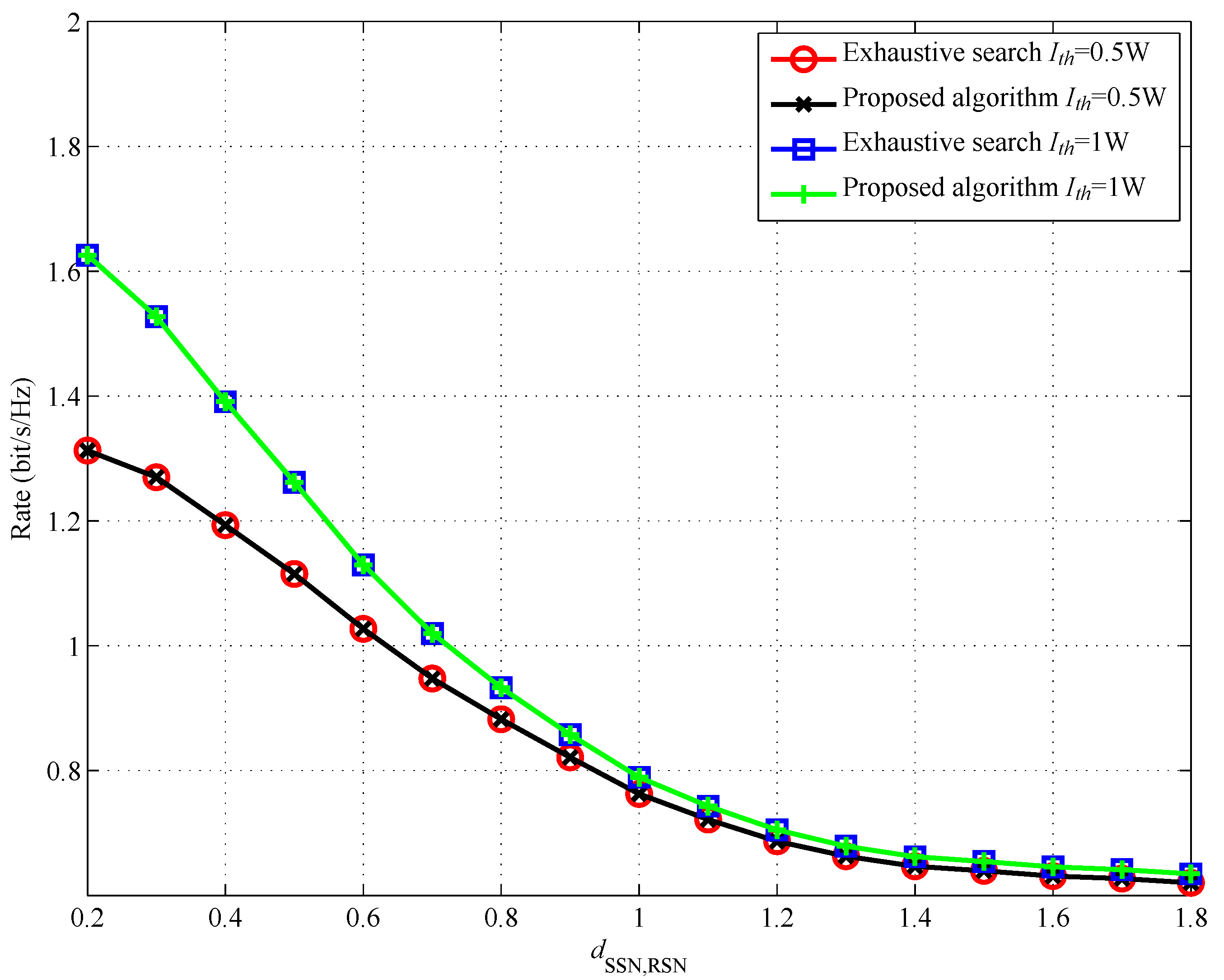
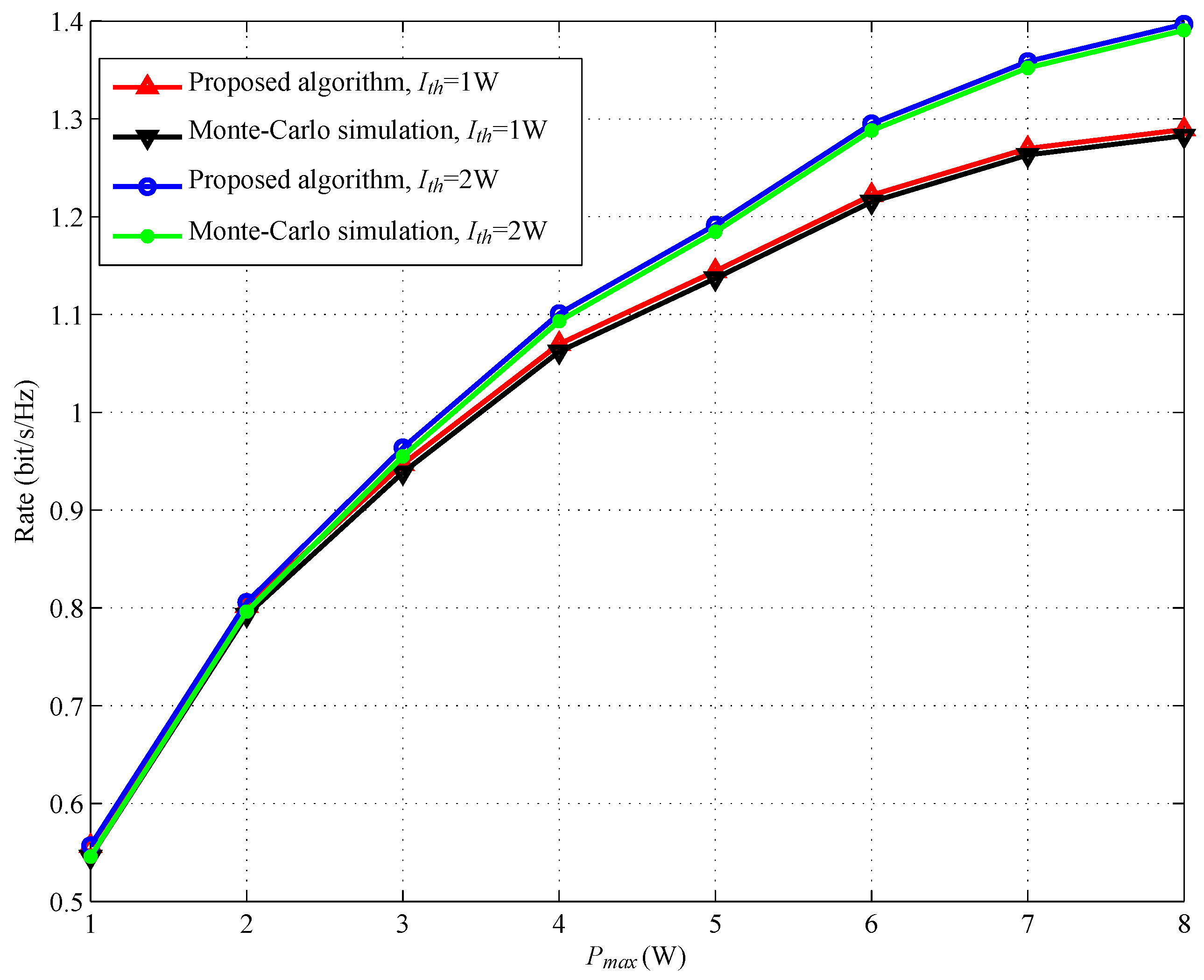
  • Finally, we show that there is no performance gap between our proposed algorithm and exhaustive search method.
The remainder of this paper is organized as follows. Section 2 describes the system model and the problem formulation for the underlay CSN with SWIPT-enabled relay node. An algorithm to solve the transmit power and power splitting ratio joint optimization problem is given in Section 3. Simulation results are presented in Section 4. Finally, Section 5 concludes the paper.

2. System Model and Problem Formulation
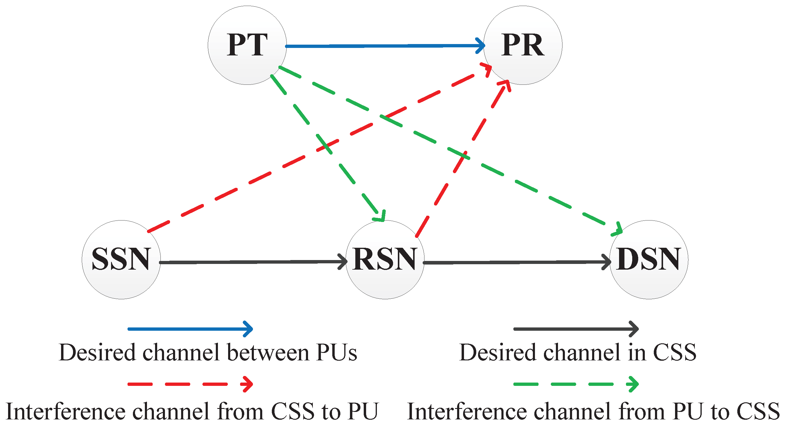
2.1. System Model

We consider an underlay CSN consisting of a primary system and a cognitive sensor system (CSS), as illustrated in Figure 1. The primary system contains a primary transmitter (PT) and a primary receiver (PR), and the CSS contains a source sensor node (SSN) and a destination sensor node (DSN). There is no direct link between SSN and DSN. Thus, the signal transmitted from SSN to DSN is forwarded by a relay sensor node (RSN).
All the terminals are equipped with one single antenna. The transmissions from CSS will cause interference to PR. At the same time, the transmit signals from PT will be treated as the interference at CSS. Between any terminals u and v, the channel coefficient is denoted as h u , v , and h u , v = g u , v d u , v m / 2 , where d u , v is the distance between u and v, and m is the path loss exponent, g u , v CN 0 , μ is Rayleigh fading coefficient and μ = 1 .
The relaying communication takes place in two equal phases. During the first phase, SSN transmits the signal to RSN, and the received signal at the RSN is expressed as
y = P s x s h SSN , RSN + n a + P p x p h PT , RSN ,
where P s and P p are the transmit power of SSN and PT, respectively. x s and x p are the normalized signals transmitted by the SSN and PT, respectively. n a CN 0 , σ a 2 is the additive white Gaussian noise (AWGN) at the RSN.
The RSN splits the received signal into two parts: one part with the power splitting ratio λ ( 0 λ 1 ) is used for the energy harvesting and the other part ( 1 λ ) is used for information processing. The signal for energy harvesting can be expressed as
E = 1 2 η λ P s h SSN , RSN 2 + σ a 2 + P p h PT , RSN 2 ,
where η 0 < η < 1 is the energy conversion efficiency. Then, the transmitted power of RSN is
P r = E / 1 / 2 = η λ P s h SSN , RSN 2 + σ a 2 + P p h PT , RSN 2 .
In the second phase, RSN amplifies the received signal and forwards it to DSN. The transmitted signal of RSN is expressed as
y r = ϕ 1 λ y + n b ,
where n b CN 0 , σ b 2 is the noise caused by the signal conversion from RF band to baseband [13], and ϕ is the amplification factor of RSN, which is represented as [19]
ϕ = P r 1 λ P s | h SSN , RSN | 2 + σ a 2 + P p | h PT , RSN | 2 + σ b 2 η λ 1 λ .
In Section 4, we demonstrate the approximation by using mathematical simulation. In the second phase, the received signal at the DSN is given by
y d = y r h RSN , DSN + n c + P p x p h PT , DSN ,
where n c CN 0 , σ c 2 is AWGN at the DSN.
Substituting Labels (1), (4) and (5) into Label(6), we can obtain
y d = η λ P s h SSN , RSN h RSN , DSN x s + η λ P p h PT , RSN h RSN , DSN + P p h PT , DSN x p + η λ 1 λ h RSN , DSN 1 λ n a + n b + n c .
From Label (7), we can compute the signal-to-interference-plus-noise ratio (SINR) at the DSN as the following:
S I N R = A λ 2 + A λ B λ 2 + B + C D λ + D P s ,
where A = η h SSN , RSN 2 h RSN , DSN 2 , B = η P p h RSN , DSN 2 h PT , RSN 2 + η h RSN , DSN 2 σ a 2 , C = η h RSN , DSN 2 σ b 2 and D = P p h PT , DSN 2 + σ c 2 .
Therefore, the achievable rate at the DSN is given by
R d = 1 2 log 2 1 + S I N R .

2.2. Problem Formulation

During the first and second phase, the interference caused by SSN and RSN to PR is given by
I s = P s h SSN , PR 2 ,
I r = P r h RSN , PR 2 = η λ P s h SSN , RSN 2 + σ a 2 + P p h PT , RSN 2 h RSN , PR 2 .
Thus, the optimization problem is formulated as
O P 1 : max P s , λ R d ,
s . t . C 1 : I s I t h ,
C 2 : I r I t h ,
C 3 : 0 < P s P m a x ,
C 4 : λ [ 0 , 1 ] ,
where C 1 and C 2 denote that the interference caused by CSS to PR should not be larger than I t h . C 3 denotes that the maximum transmit power for SSN should not be larger than P m a x . C 4 shows the practical constraint of λ .
Since log ( x ) is a monotone increasing function of x, log can be omitted in the object function. Moreover, 1 is an invariant constant. Thus, O P 1 can be transformed into the following problem:
O P 2 : max P s , λ S I N R ,
s . t . C 1 , C 2 , C 3 , C 4 .

3. Joint Optimization of Transmit Power and Power Allocation Ratio

In this part, we solve the above problem with the following two steps. Firstly, we find the optimal power splitting ratio λ * with fixed transmit power P s . Then, we find the optimal transmit power P s * . We will show in the numerical results that there is no performance gap between the above solution with the exhaustive search.

3.1. Finding the λ * with Fixed P s

Taking the first derivation of Label (8) with λ , we can obtain
d S I N R d λ = A D C λ 2 2 A D λ + A D B λ 2 + B + C D λ + D 2 P s .
Obviously, the fact that d S I N R d λ is positive or negative only depends on the value of f λ = A D C λ 2 2 A D λ + A D , as P s and B λ 2 + B + C D λ + D 2 are always positive. Moreover, it is easy to find that whether f λ is positive or negative not only relies on the constraint of λ , but also the relative values of C and D. Thus, λ * can be obtained by analyzing the relative values of C and D with the constraint of λ .
Case 1 when D < C
Apparently, f λ is a quadratic function of λ , and we can find
f 1 = A ( D C ) 2 A D + A D = A C < 0 ,
f 0 = A D > 0 .
The discriminant of corresponding quadratic equation can be written as:
Δ = 2 A D 2 4 A D C A D = 4 A 2 C D > 0 .
Thus, the equation has two different roots and can be respectively written as
λ 1 = 2 A D 2 A C D 2 A D C = D C D D C ,
λ 2 = 2 A D + 2 A C D 2 A D C = D + C D D C .
From Labels (18) and (19), we can find that 0 < λ 1 < 1 and λ 2 < 0 . From Labels (15) and (16), we can find that there is only one maxima that lies between 0 , 1 , and the position is at λ = λ 1 . Thus, it is obvious that, for λ < λ 1 , S I N R is a monotone increasing function of λ ; and, for λ > λ 1 , S I N R is a monotone decreasing function of λ . Meanwhile, we should consider the constraint C 2 . From the constraint C 2 , we can obtain
λ λ t h = I t h E P s + F ,
where E = η h SSN , RSN 2 h RSN , PR 2 , F = η σ a 2 + P p h PT , RSN 2 h RSN , PR 2 . Thus, if λ t h λ 1 , λ * = λ t h ; otherwise, λ * = λ 1 .
Case 2 when D > C
With the similar analysis in Case 1, the optimal value of λ can be obtained as
λ * = λ 1 = D C D D C , if λ t h > λ 1 , λ t h = I t h E P s + F , if λ t h λ 1 .
Case 3 when D = C
Apparently, f λ is a linear function of λ . We can find
f 1 = 2 A D + A D = A D < 0 ,
f 0 = A D > 0 ,
f 1 2 = 2 A D * 1 2 + A D = 0 .
From Labels (22)–(24), we can find that, for λ < 1 2 , S I N R is a monotone increasing function of λ , and, for λ > 1 2 , S I N R is a monotone decreasing function of λ . Meanwhile, we also should consider the constraint C 2 as above. Then, if λ t h 1 2 , λ * = λ t h ; otherwise, λ * = 1 2 .
Concluded from the above analyses in Case 1 to Case 3, we can obtain that when D C , the optimal value of λ is
λ * = λ 1 = D C D D C , if λ t h > λ 1 , λ t h = I t h E P s + F , if λ t h λ 1 ,
when D = C , the optimal value of λ is
λ * = 1 2 , if λ t h > 1 2 , λ t h = I t h E P s + F , if λ t h 1 2 .

3.2. Finding P s *

From Section 3.1, we can find that λ * may have three different values, which are λ 1 , 1 2 and λ t h . The optimal power allocation is obtained depending on the different values of λ * .
Case 1 when λ * = λ 1 , it should satisfy D C and λ t h > λ 1 .
Substituting λ * = λ 1 = D C D D C into Label (8), we can obtain
S I N R = A C + A D 2 A C D B C + B D 2 C D + C 2 + D 2 2 B C D P s = A ( C D ) 2 B ( C D ) 2 + ( C D ) 2 P s .
To satisfy the constraints C 1 , C 2 and C 3 , we can obtain
P s P s C 1 = I t h h SSN , PR 2 ,
P s P s C 2 = I t h D C η D C D h RSN , PR 2 σ a 2 P p h PT , RSN 2 h SSN , RSN 2 ,
P s P s C 3 = P m a x .
From Label (27), we can find that S I N R is a monotone increasing function of P s . Thus, if  min P s C 1 , P s C 3 P s C 2 , S I N R obtains the maximum value when P s = P s C 2 . However, when P s = P s C 2 , we can get λ t h = λ 1 , which does not satisfy the condition that λ 1 < λ t h . Thus, when λ * = λ 1 , we can get that min P s C 1 , P s C 3 < P s C 2 , and P s 0 , min P s C 1 , P s C 3 . Thus, when P s = min P s C 1 , P s C 3 , S I N R  obtains the maximum value. The optimal value of P s can be obtained as
P s * = min P s C 1 , P s C 3 .
Case 2 when λ * = 1 2 , it should satisfy D = C and λ t h > 1 2 .
With a similar analysis in Case 1, the optimal value of P s can be obtained as
P s * = min P s C 1 , P s C 3 .
Case 3 when λ * = λ t h
From Labels (25) and (26), we can find that, in this case, it will have two different conditions.
Condition 1 D C and λ t h λ 1
Substituting λ = λ t h = I t h E P s + F into Label (8), we can get
S I N R = A I t h E P s + F 2 + A I t h E P s + F B I t h E P s + F 2 + B + C D I t h E P s + F + D P s = α P s 2 + β P s γ P s 2 + θ P s + ω ,
where α = A E I t h , β = A F I t h A I t h 2 , γ = D E 2 , θ = 2 D E F + B + C D E I t h , and ω = D F 2 + B + C D F I t h B I t h 2 .
We can find that the constraint C 2 is satisfied when λ * = λ t h . Moreover, to satisfy constraints C 1 and C 3 , we can obtain
P s P s C 1 = I t h h SSN , PR 2 ,
P s P s C 3 = P m a x .
To satisfy the condition λ t h λ 1 , we can obtain
P s P s C 4 = I t h D C η D C D h RSN , PR 2 σ a 2 P p h PT , RSN 2 h SSN , RSN 2 .
If min P s C 1 , P s C 3 < P s C 4 , then, P s min P s C 1 , P s C 3 < P s C 4 , which does not satisfy the condition P s P s C 4 . Thus, when λ * = λ t h , we can obtain that min P s C 1 , P s C 3 P s C 4 . Then, we can obtain P s P s C 4 , min P s C 1 , P s C 3 .
Take the first derivation of Label (33) with P s , we can obtain
d S I N R d P s = 2 α P s + β γ P s 2 + θ P s + ω α P s 2 + β P s 2 γ P s + θ γ P s 2 + θ P s + ι 2 = α θ β γ P s 2 + 2 α ω P s + β ω γ P s 2 + θ P s + ω 2 .
Obviously, the fact that d S I N R d P s is positive or negative only depends on the value of f P s = α θ β γ P s 2 + 2 α ω P s + β ω . f P s is a quadratic function of P s . We can find
α θ β γ = A E I t h 2 D E F + B + C D E I t h A F I t h A I t h 2 D E 2 = A D E 2 F I t h + A B + C E 2 I t h 2 > 0 .
Thus, the opening of f P s is up. The symmetry axis can be expressed as
P s = 2 α ω 2 α θ β γ = α ω α θ β γ .
The discriminant of corresponding quadratic equation can be written as
Δ = 2 α ω 2 4 α θ β γ β ω = 4 A 2 C E 2 I t h 4 ω .
We can find that the shape of f P s is related to the value of ω .
(1) when ω 0 , f P s is shown in Figure 2.
In this situation, α ω α θ β γ 0 , the symmetry axis is at a nonnegative axle. If β = A F I t h A I t h 2 0 , we can obtain F I t h , then ω = D F 2 + B + C D F I t h B I t h 2 C I t h > 0 , which will not satisfy the condition that ω 0 . Thus, β = A F I t h A I t h 2 < 0 , and then we can obtain Δ = 4 A 2 C E 2 I t h 4 ω 0 . In addition, we can obtain β ω 0 . Thus, we can find that there is one zero point or none. Thus, when  ω 0 , we can obtain f P s 0 , d S I N R d P s 0 , S I N R is a monotone increasing function of P s . When P s = min P s C 1 , P s C 3 , S I N R obtains the maximum value. Thus, the optimal value of P s can be obtained as
P s * = min P s C 1 , P s C 3 .
(2) when ω > 0
In this situation, α ω α θ β γ < 0 , the symmetry axis is at the negative axle. Moreover, Δ = 4 A 2 C E 2 I t h 4 ω > 0 , there are two zero points, which are P s 1 = α ω + 4 A 2 C E 2 I t h 4 ω 2 α θ β γ and P s 2 = α ω 4 A 2 C E 2 I t h 4 ω 2 α θ β γ , respectively. However, the shape of function f P s is also related to the value of β .
(i) when β 0 , f P s is shown in Figure 3.
In this situation, β ω 0 , we can obtain f P s 0 , d S I N R d P s 0 , S I N R is a monotone increasing function of P s . Thus, when P s = min P s C 1 , P s C 3 , S I N R obtains the maximum value. Thus, the optimal value of P s can be obtained as
P s * = min P s C 1 , P s C 3 .
(ii) when β < 0
In this situation, β ω < 0 . When P s 1 < P s C 4 , as shown in Figure 4a, we can obtain f P s > 0 , d S I N R d P s > 0 , and S I N R is a monotone increasing function of P s . Thus, when P s = min P s C 1 , P s C 3 , S I N R  obtains the maximum value. Thus, the optimal value of P s can be obtained as
P s * = min P s C 1 , P s C 3 ,
when P s C 4 P s 1 min P s C 1 , P s C 3 , as shown in Figure 4b. When P s P s C 4 , P s 1 , we can obtain f P s 0 , d S I N R d P s 0 , S I N R is a monotone decreasing function of P s ; when P s P s 1 , min P s C 1 , P s C 3 , we can obtain f P s > 0 , d S I N R d P s > 0 , S I N R is a monotone increasing function of P s . Thus, the optimal value of P s can be obtained as
P s * = min P s C 1 , P s C 3 , if S I N R min P s C 1 , P s C 3 S I N R P s C 4 , P s C 4 , if S I N R min P s C 1 , P s C 3 < S I N R P s C 4 ,
when min P s C 1 , P s C 3 < P s 1 , as shown in Figure 4c, we can obtain f P s < 0 , d S I N R d P s < 0 , S I N R is a monotone decreasing function of P s . Thus, when P s = P s C 4 , S I N R obtains the maximum value. Thus, the optimal value of P s can be obtained as
P s * = P s C 4 .
Condition 2 D = C and λ t h 1 2
To satisfy the condition λ t h 1 2 , we can obtain
P s P s C 5 = 2 I t h η h RSN , PR 2 σ a 2 P p h PT , RSN 2 h SSN , RSN 2 .
Then, with the similar analysis in Condition 1, we can obtain
P s * = P s C 5 , if 1 . ω > 0 , β < 0 , P s C 5 P s 1 min P s C 1 , P s C 3 and S I N R min P s C 1 , P s C 3 ) < S I N R ( P s C 5 , 2 . ω > 0 , β < 0 and min P s C 1 , P s C 3 < P s 1 , min P s C 1 , P s C 3 , otherwise .
Concluded from the above analyses in Case 1 to Case 3, we can obtain that when λ * = λ 1 or λ * = 1 2 , the optimal value of P s is
P s * = min P s C 1 , P s C 3 ,
when λ * = λ t h ,
(i) if D C , the optimal value of P s is
P s * = P s C 4 , if 1 . ω > 0 , β < 0 , P s C 4 P s 1 min P s C 1 , P s C 3 and S I N R min P s C 1 , P s C 3 ) < S I N R ( P s C 4 , 2 . ω > 0 , β < 0 and min P s C 1 , P s C 3 < P s 1 , min P s C 1 , P s C 3 , otherwise
(ii) if D = C , the optimal value of P s is
P s * = P s C 5 , if 1 . ω > 0 , β < 0 , P s C 5 P s 1 min P s C 1 , P s C 3 and S I N R min P s C 1 , P s C 3 ) < S I N R ( P s C 5 , 2 . ω > 0 , β < 0 and min P s C 1 , P s C 3 < P s 1 , min P s C 1 , P s C 3 , otherwise
Based on the above analysis, Algorithm 1 presents the process of the proposed algorithm for joint optimization problem.
Algorithm 1 Proposed Algorithm for Joint Optimization Problem.
1.if D C
2.if λ t h > λ 1 then
3. λ * = λ 1 and P s * = min P s C 1 , P s C 3
4.else
5.if ω > 0 , β < 0 , P s C 4 P s 1 min P s C 1 , P s C 3 , S I N R min P s C 1 , P s C 3 ) < S I N R ( P s C 4 or ω > 0 , β < 0 , min P s C 1 , P s C 3 < P s 1 then
6. λ * = λ t h and P s * = P s C 4
substituting P s * into λ t h obtains the optimal value of λ *
7.else
8. λ * = λ t h and P s * = min P s C 1 , P s C 3
substituting P s * into λ t h obtains the optimal value of λ *
9.end if
10.end if
11.else
12.if λ t h > 1 2 then
13. λ * = 1 2 and P s * = min P s C 1 , P s C 3
14.else
15.if ω > 0 , β < 0 , P s C 5 P s 1 min P s C 1 , P s C 3 , S I N R min P s C 1 , P s C 3 ) < S I N R ( P s C 5 or ω > 0 , β < 0 , min P s C 1 , P s C 3 < P s 1 then
16. λ * = λ t h and P s * = P s C 5
substituting P s * into λ t h obtains the optimal value of λ *
17.else
18. λ * = λ t h and P s * = min P s C 1 , P s C 3
substituting P s * into λ t h obtains the optimal value of λ *
19.end if
20.end if
21.end if

4. Simulation Results and Discussion

Unless otherwise stated, we assume that the path loss exponent m = 3 , the energy harvesting efficiency η = 0 . 8 , the distance d SSN , RSN + d RSN , DSN = 2 , and d PT , RSN = d PT , DSN = d SSN , PR = d RSN , PR = 2 , the PT transmission power P p = 2 W , the maximal SSN transmission power P m a x = 2 W . For simplicity, noise variances σ a 2 = σ b 2 = σ c 2 = 0 . 01 . All simulation results are averaged over 10,000 channel realizations.
Figure 5 shows the achievable rate of the cognitive sensor system versus d SSN , RSN . It can be observed from Figure 5 that there is no performance gap between our proposed algorithm and the exhaustive search method. In Figure 5, we can find that the achievable rate becomes larger when RSN moves closer to SSN, which is due to the fact that when RSN is located closer to SSN, it can harvest more power in the first slot to help forward SSN’s signal to DSN in the second slot. We can also observe from Figure 5 that, with larger I t h , SSN can achieve a larger rate. This is because, with a larger I t h , PR can tolerate a larger interference from the cognitive sensor network. Then, SSN and RSN can use more power to transmit the signal, which can be illustrated in Figure 6 and Figure 7.
Figure 6 and Figure 7 show the achievable rate versus I t h with different power splitting ratio λ and with different transmit power P s , respectively. The distance between SSN and RSN, d SSN , RSN , is set to be 1. In Figure 6, we can find that SSN obtains the maximum rate when RSN uses the optimal power splitting ratio λ * . In Figure 7, we can also observe that SSN will obtain the maximum rate when RSN uses the optimal transmit power P s * .
Figure 8 shows the achievable rate versus η with different I t h and P m a x . The distance between SSN and RSN, d SSN , RSN , is set to be 1. In Figure 8, we can find that the achievable rate increases with the η . This is due to the fact that, with larger η , RSN can harvest more energy to help forward the SSN information, which leads to a larger achievable rate at DSN. Figure 9 shows the optimal λ versus η with different d SSN , RSN . The interference threshold I t h is set to be 1 W. It can be observed from Figure 9 that λ * decreases with the increase of η . Then, RSN can use more energy to forward SSN information, which also illustrates a larger achievable rate as shown in Figure 8.
Figure 10 shows the achievable rate versus P m a x with different I t h . It can be observed from Figure 10 that the performance gap between the proposed algorithm and Monte Carlo simulation is very small, which illustrates the approximation in Label (5). We also can observe from Figure 10 that the achievable rate increases with the maximal SSN transmission power P m a x .
Figure 11 shows the optimal λ versus I t h with different d SSN , RSN . The maximal transmit power of SSN, P m a x is set to be 3 W , the PT transmission power P p = 3 W . It can be observed from Figure 11 that λ * becomes larger with the increase of I t h . When I t h is sufficiently small, and we can find that P s C 1 P s C 3 , and λ * = λ t h , P s * = P s C 1 . As I t h increases, P s C 1 becomes larger, when P s C 1 > P s C 3 , we can find that λ * = λ t h , P s * = P s C 3 , and λ * linearly increases with the increase of I t h . However, when I t h reaches a certain level, λ * becomes to be a constant, which equals λ 1 .

5. Conclusions

In this paper, we investigated the performance of underlay CSNs with SWIPT-enabled relay node. Considering the constraints of interference power at PR and the transmit power at SSN, we propose an algorithm to solve the transmit power and the power splitting ratio joint optimization problem. Meanwhile, the closed-form expressions for λ * and P s * are derived. It is shown that there is no performance gap between our proposed algorithm and the exhaustive search method, while the complexity can be reduced.

Acknowledgments

This work was supported by the National Natural Science Foundation of China under Grant Nos. 61402416 and 61601221, and the China Postdoctoral Science Foundations under Grant No. 2017M612027.

Author Contributions

Weidang Lu and Yuanrong Lin conceived and designed the SWIPT-based CSN model; Hong Peng and Tian Nan optimized the proposed models; Xin Liu performed the simulations of the model; and Weidang Lu wrote the paper.

Conflicts of Interest

The authors declare no conflict of interest.

References

  1. Liu, Y.; Mousavifar, S.A.; Deng, Y.; Leung, C.; Elkashlan, M. Wireless energy harvesting in a cognitive relay network. IEEE Trans. Wirel. Commun. 2016, 15, 2498–2508. [Google Scholar] [CrossRef]
  2. Akan, O.B.; Karli, O.B.; Ergul, O. Cognitive radio sensor networks. IEEE Netw. 2009, 23, 34–40. [Google Scholar] [CrossRef]
  3. Zhang, D.; Chen, Z.; Ren, J.; Ning, Z.; Awad, K.M.; Zhou, H.; Shen, X. Energy harvesting-aided spectrum sensing and data transmission in heterogeneous cognitive radio sensor network. IEEE Trans. Veh. Technol. 2017, 66, 831–843. [Google Scholar] [CrossRef]
  4. Sudevalayam, S.; Kulkarni, P. Energy harvesting sensor nqodes: survey and implications. IEEE Commun. Surv. Tutor. 2011, 13, 443–461. [Google Scholar] [CrossRef]
  5. Ho, C.K.; Zhang, R. Optimal energy allocation for wireless communications with energy harvesting constraints. IEEE Trans. Signal Process. 2012, 60, 4808–4818. [Google Scholar] [CrossRef]
  6. Chalasani, S.; Conrad, J. A survey of energy harvesting sources for embedded systems. In Proceedings of the IEEE SoutheastCon, Huntsville, AL, USA, 3–6 April 2008; pp. 442–447. [Google Scholar]
  7. Lu, X.; Wang, P.; Niyato, D.; Kim, D.I.; Han, Z. Wireless networks with RF energy harvesting: A contemporary survey. IEEE Commun. Surv. Tutor. 2015, 17, 757–789. [Google Scholar] [CrossRef]
  8. Varshney, L.R. Transporting information and energy simultaneously. In Proceedings of the Information Theory, Toronto, ON, Canada, 6–11 July 2008; pp. 1612–1616. [Google Scholar]
  9. Zhou, X.; Zhang, R.; Ho, C.K. Wireless information and power transfer: architecture design and rate-energy tradeoff. IEEE Trans. Commun. 2013, 61, 4754–4767. [Google Scholar] [CrossRef]
  10. Liu, L.; Zhang, R.; Chua, K.C. Wireless information transfer with opportunistic energy harvesting. IEEE Trans. Wirel. Commun. 2013, 12, 288–300. [Google Scholar] [CrossRef]
  11. Lee, S.; Huang, K.; Zhang, R. Cognitive energy harvesting and transmission from a network perspective. In Proceedings of the 2012 IEEE Communication Systems, Singapore, 21–23 November 2012; pp. 225–229. [Google Scholar]
  12. Guo, S.; Wang, F.; Yang, Y.; Xiao, B. Energy-efficient cooperative for simultaneous wireless information and power transfer in clustered wireless sensor networks. IEEE Trans. Commun. 2015, 63, 4405–4417. [Google Scholar] [CrossRef]
  13. Nasir, A.A.; Zhou, X.; Durrani, S.; Kennedy, R.A. Relaying protocols for wireless energy harvesting and information processing. IEEE Trans. Wirel. Commun. 2013, 12, 3622–3636. [Google Scholar] [CrossRef]
  14. Ding, Z.G.; Esnaola, I.; Sharif, B.; Poor, H.V. Wireless information and power transfer in cooperative networks with spatially random relays. IEEE Trans. Wirel. Commun. 2014, 13, 4400–4453. [Google Scholar] [CrossRef]
  15. Mousavifar, S.A.; Liu, Y.; Leung, C.; Elkashlan, M.; Duong, T.Q. Wireless energy harvesting and spectrum sharing in cognitive radio. In Proceedings of the IEEE 80th Vehicular Technology Conference, Vancouver, BC, Canada, 14–17 September 2014; pp. 1–5. [Google Scholar]
  16. Lu, X.; Xu, W.; Li, S.; Liu, Z.; Lin, J. Simultaneous wireless information and power transfer for cognitive two-way relaying networks. In Proceedings of the Personal, Indoor, and Mobile Radio Communication (PIMRC), Washington, DC, USA, 2–5 September 2014; pp. 748–752. [Google Scholar]
  17. Im, G.; Lee, J.H. Outage probability of underlay cognitive radio networks with SWIPT-enabled relay. In Proceedings of the IEEE 82nd Vehicular Technology Conference, Boston, MA, USA, 6–9 September 2015; pp. 1–5. [Google Scholar]
  18. Singh, S.; Modem, S.; Prakriya, S. Optimization of cognitive two-way networks with energy harvesting relays. IEEE Commun. Lett. 2017, 21, 1381–1384. [Google Scholar] [CrossRef]
  19. Ju, M.; Kim, I.M. Relay selection with ANC and TDBC protocols in bidirectional relay networks. IEEE Trans. Commun. 2010, 58, 3500–3511. [Google Scholar] [CrossRef]
Figure 1. System model.
Sensors 17 02093 g001
Figure 2. The image of f P s when ω 0 .
Sensors 17 02093 g002
Figure 3. The image of f P s when ω > 0 , β 0 .
Sensors 17 02093 g003
Figure 4. The image of f P s when ω > 0 , β < 0 . (a) the image of f P s when ω > 0 , β < 0 and P s 1 < P s C 4 ; (b) the image of f P s when ω > 0 , β < 0 and P s C 4 P s 1 min P s C 1 , P s C 3 ; (c) the image of f P s when ω > 0 , β < 0 and min P s C 1 , P s C 3 < P s 1 .
Sensors 17 02093 g004
Figure 5. Achievable rate versus d SSN , RSN .
Sensors 17 02093 g005
Figure 6. Achievable rate for various λ versus I t h .
Sensors 17 02093 g006
Figure 7. Achievable rate for various P s versus I t h .
Sensors 17 02093 g007
Figure 8. Achievable rate versus η .
Sensors 17 02093 g008
Figure 9. The optimal value of λ versus η .
Sensors 17 02093 g009
Figure 10. Achievable rate versus P max .
Sensors 17 02093 g010
Figure 11. The optimal value of λ versus I t h .
Sensors 17 02093 g011

