Experimental Characterization of Close-Emitter Interference in an Optical Camera Communication System

 , and
, and 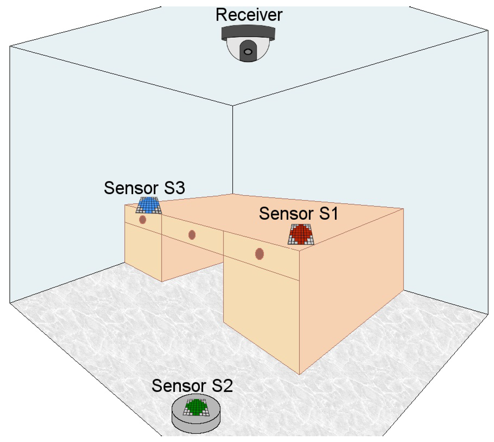
Abstract
:1. Introduction
2. Theoretical Fundaments
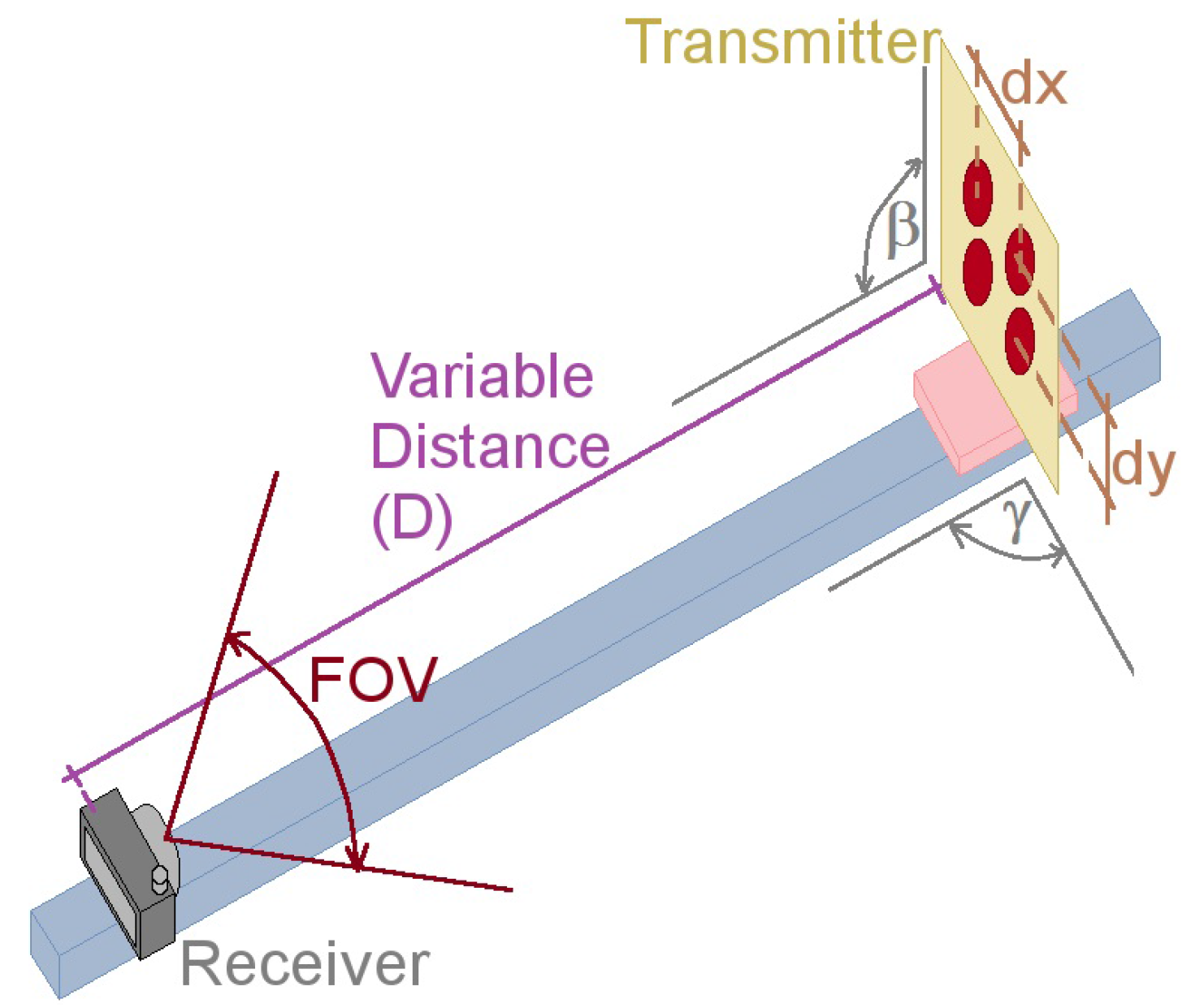
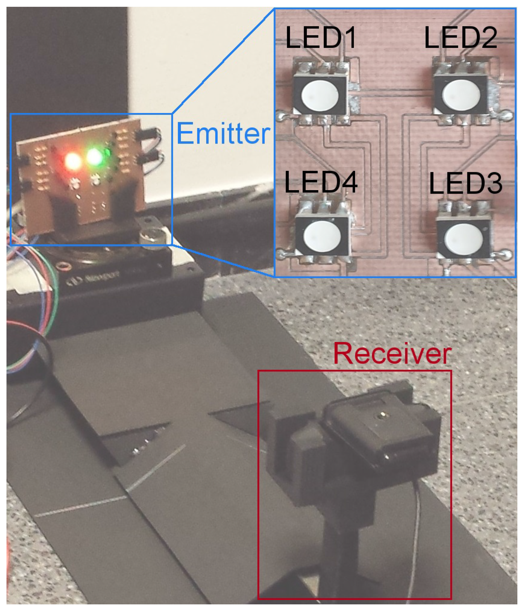
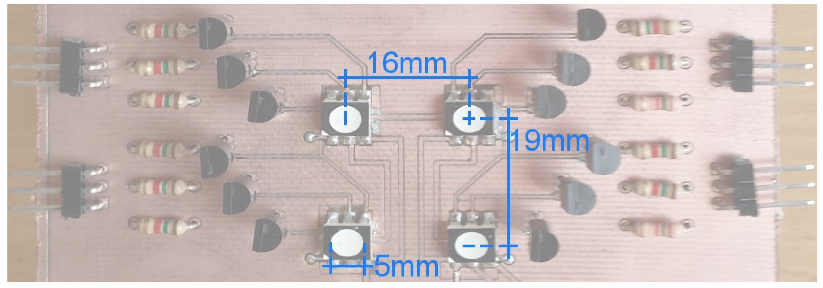
3. Experimental Design
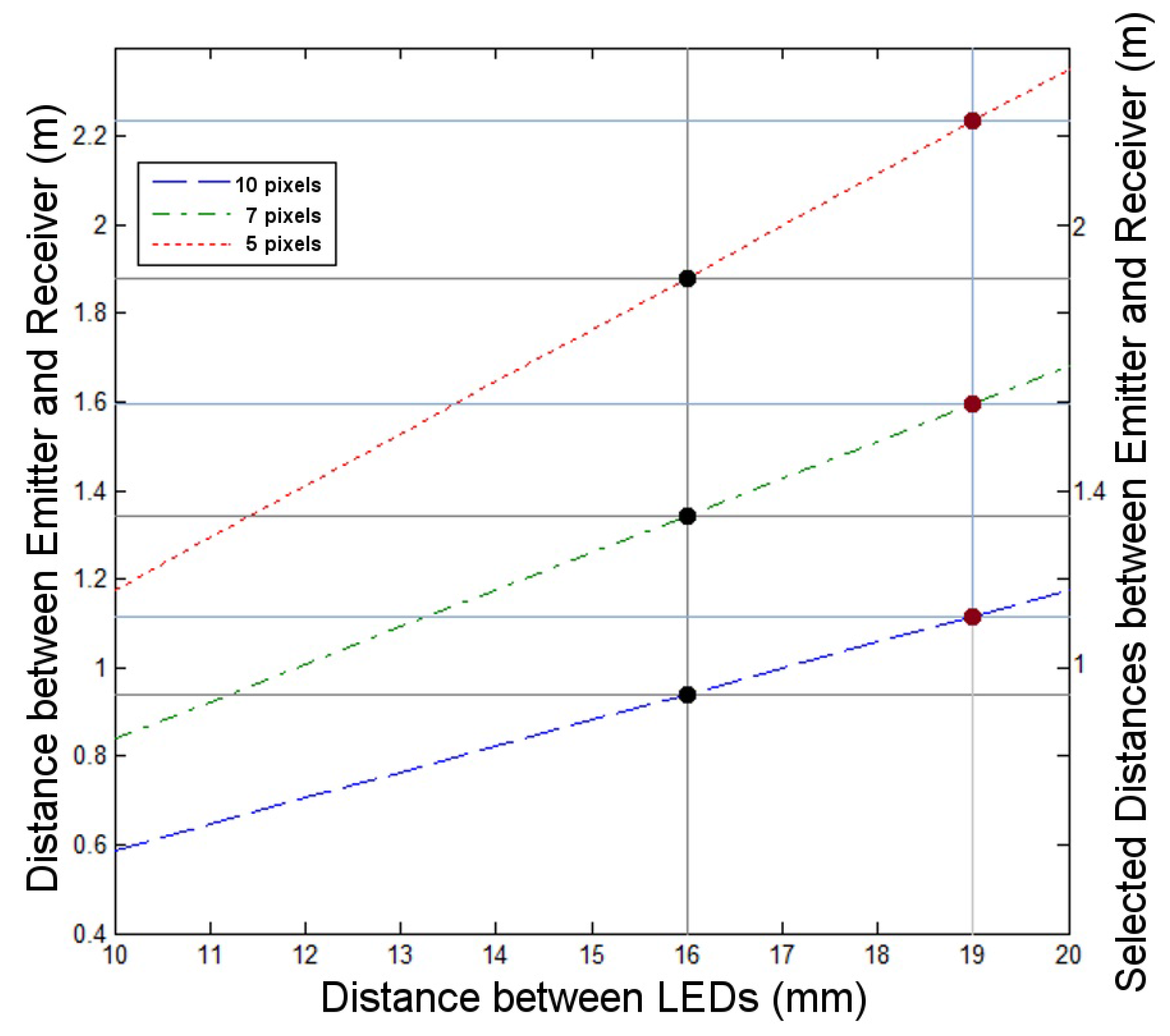
3.1. Equation Validation
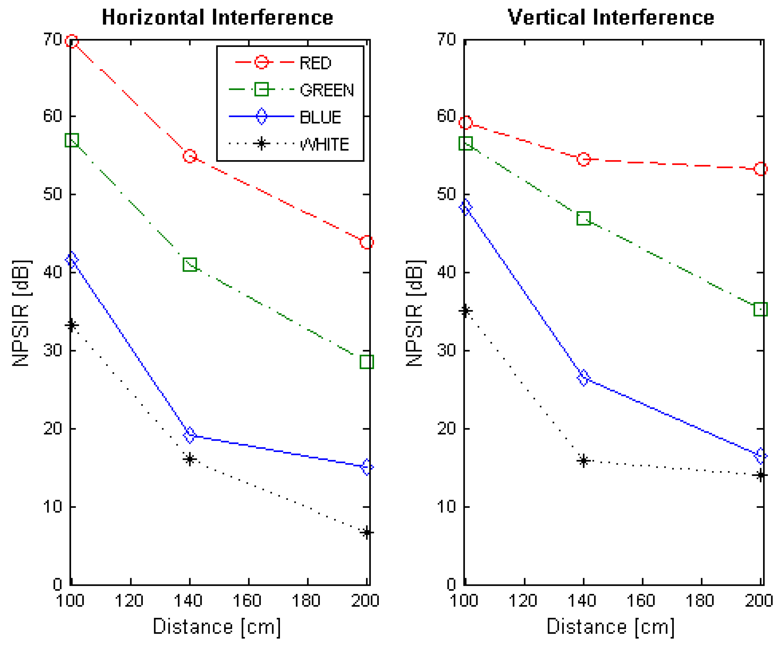
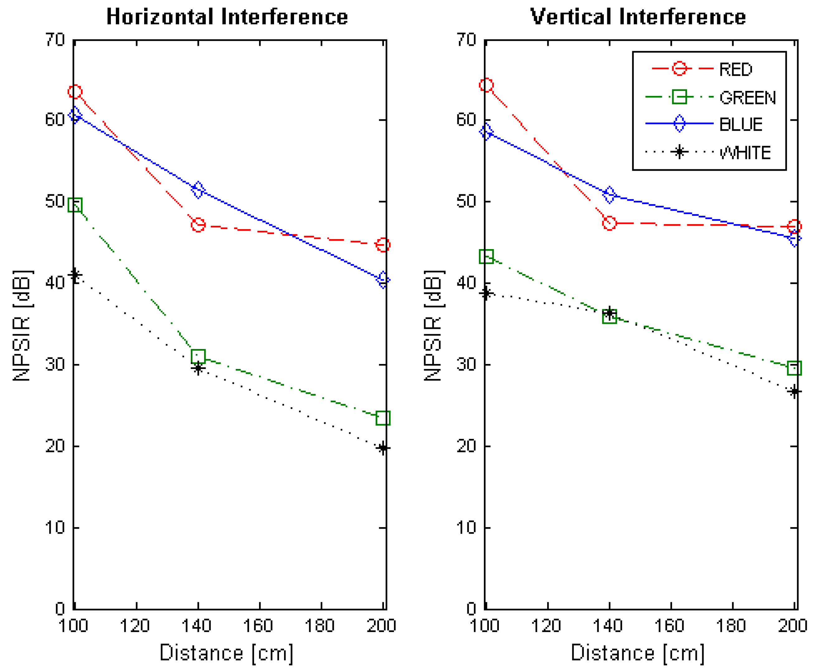
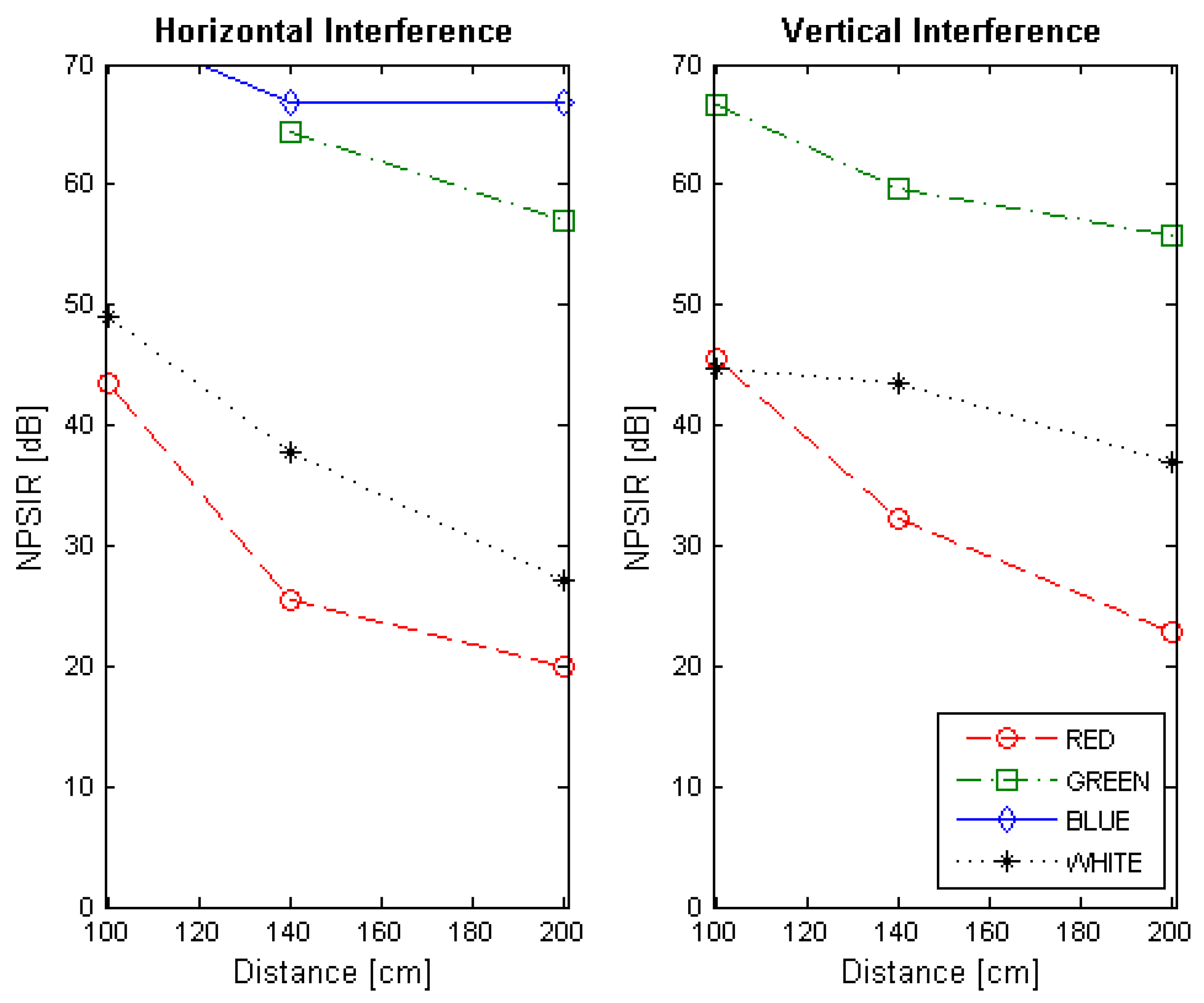
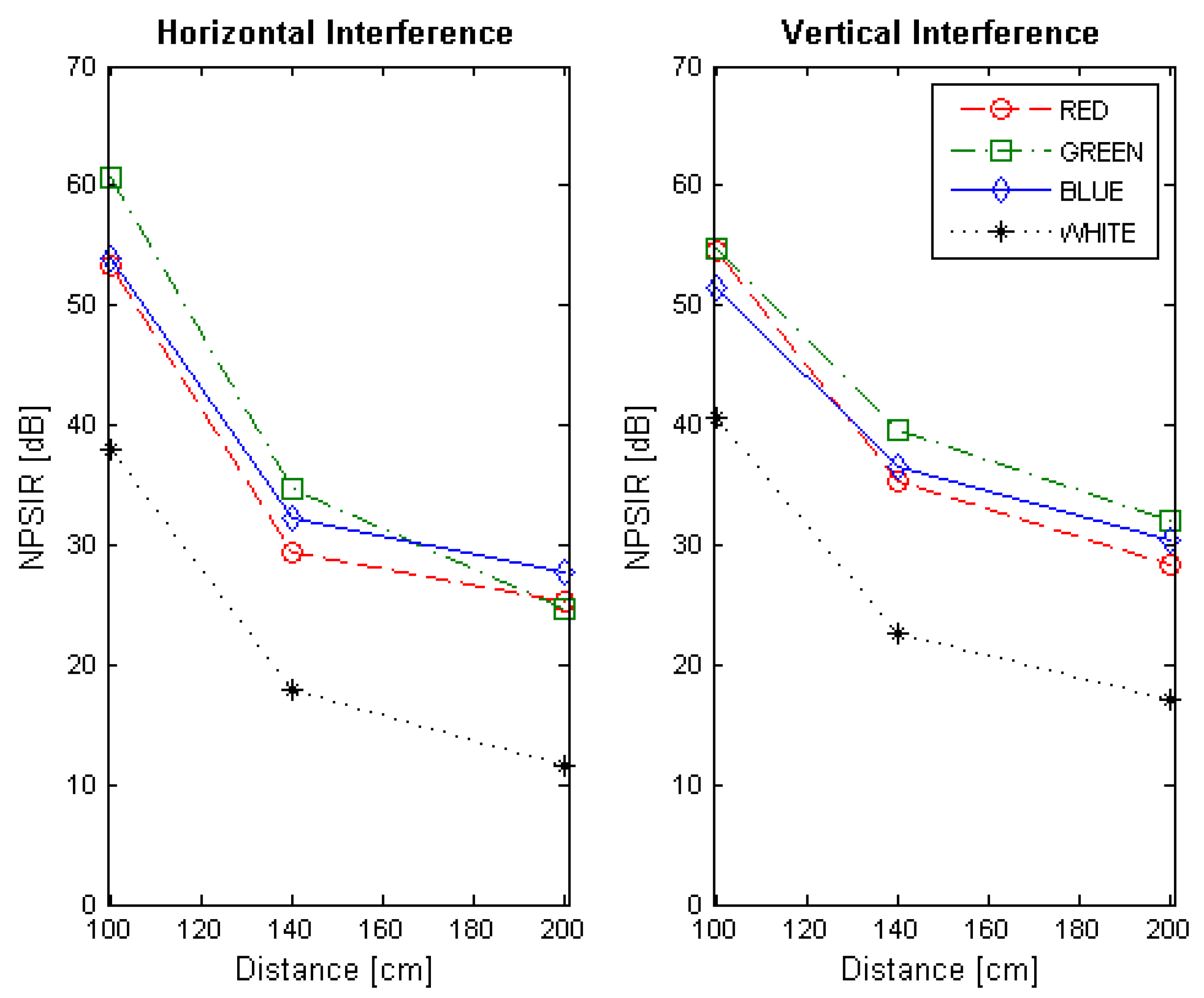
3.2. Optical Interference
- Distance for perfect spatial separation: 100 cm.
- Distance for limited spatial separation: 140 cm.
- Distance for critical spatial separation: 200 cm.
- Only one LED at the time (four combinations).
- Two horizontal LEDs at the time (two combinations).
- Two vertical LEDs at the time (two combinations).
- Two diagonal LEDs at the time (two combinations).
- Four LEDs at the time (one combination).
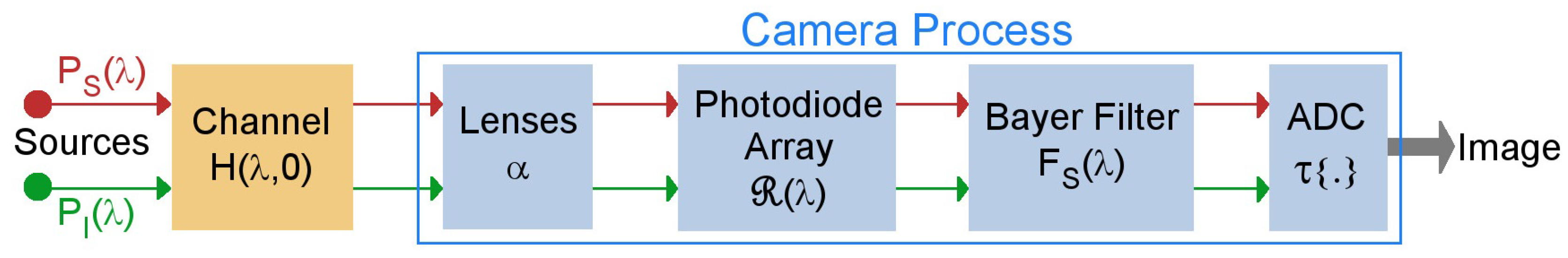
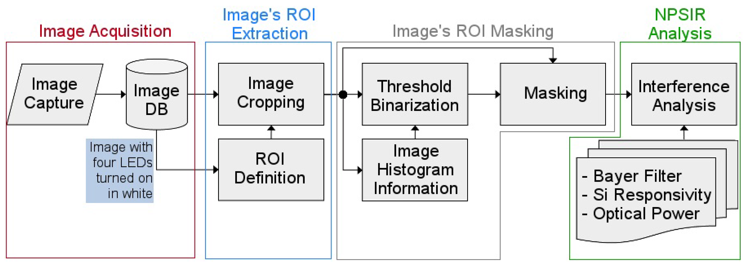
3.3. Image Acquisition
3.4. Image’s ROI Extraction
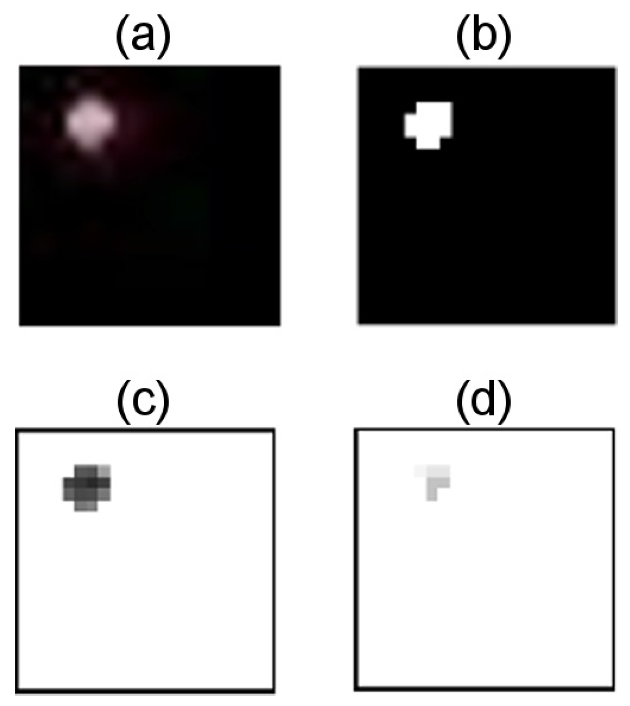
3.5. Image’s ROI Masking
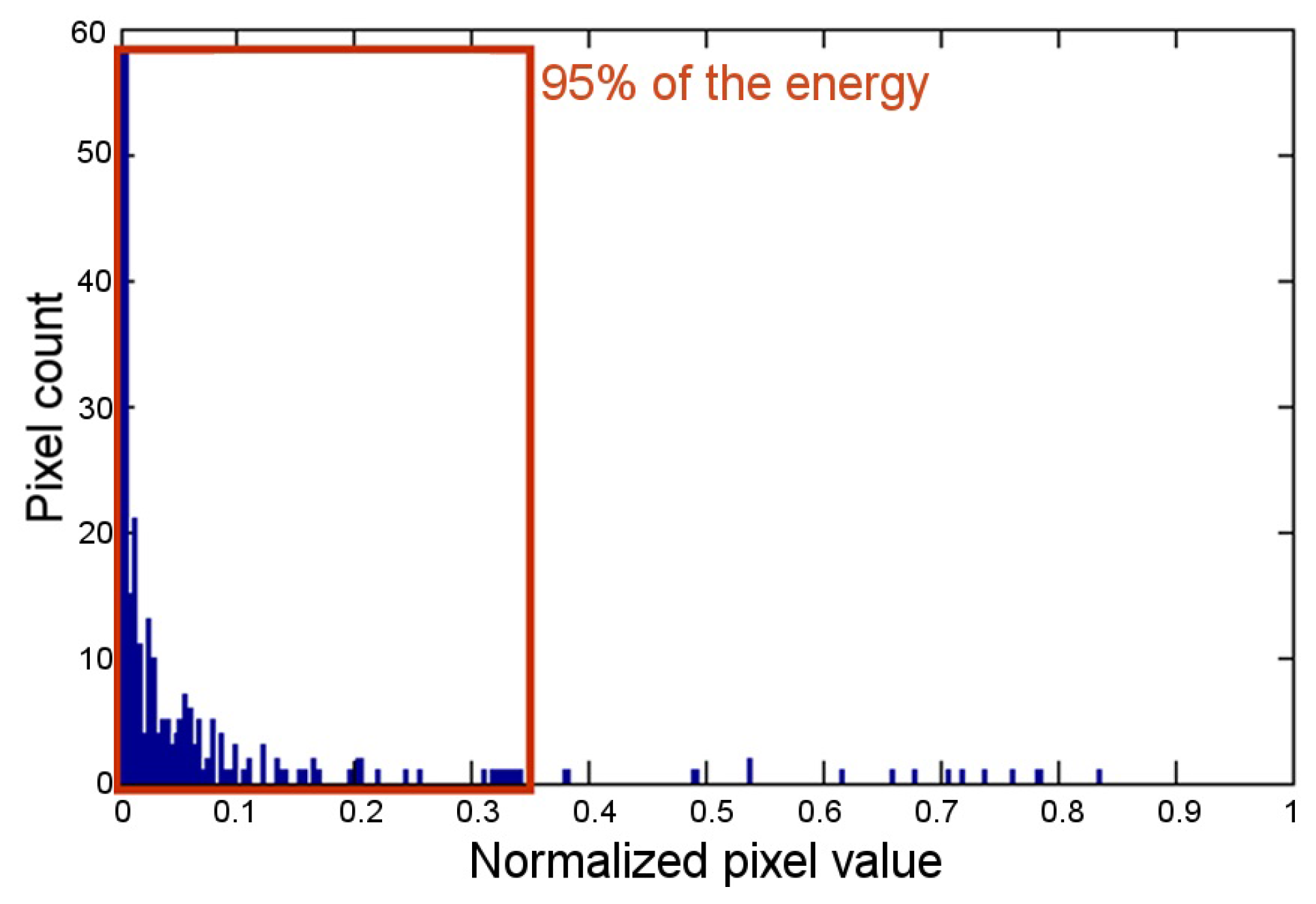
3.6. NPSIR Analysis
4. Experimental Results
5. Wireless Sensor Network Simulations
Simulation Results
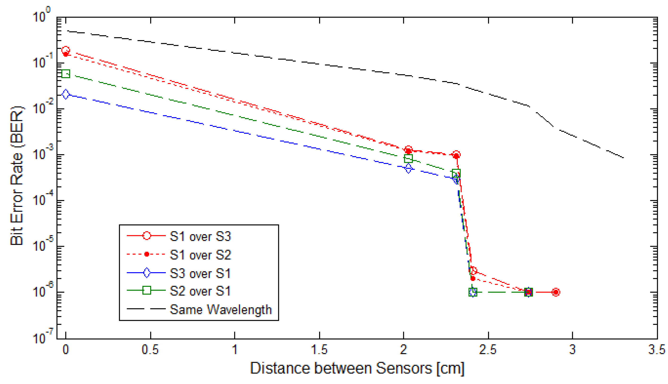
- No distance between the LED matrices so the ROI is affected by the two overlapping sources equally,
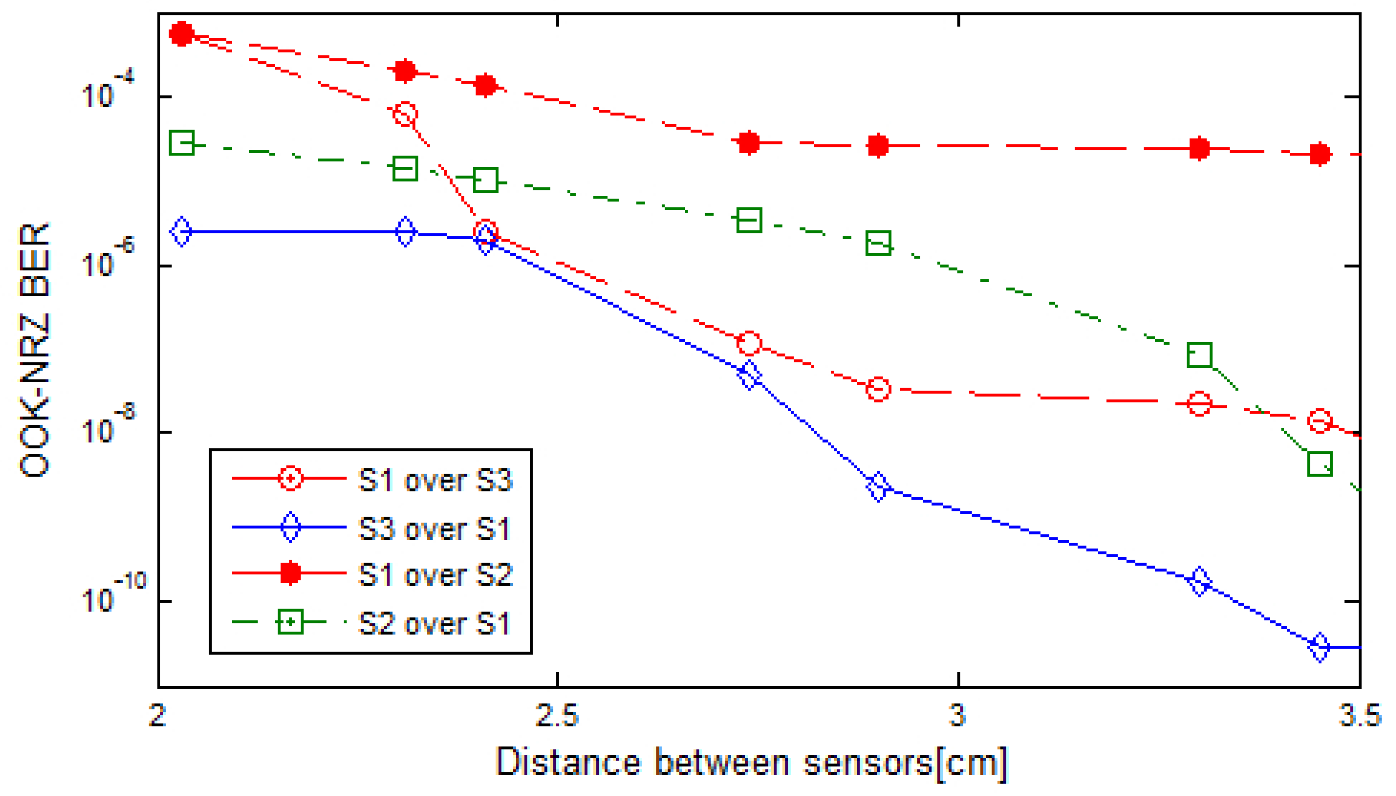
- Distance between the LED matrices is greater than 2.00 cm and the two sources transmitted in the same wavelength, and
- Distance between the LED matrices is greater than 2.00 cm and the two sources transmitted with a different wavelength.
6. Conclusions
Acknowledgments
Author Contributions
Conflicts of Interest
Abbreviations
| ADC | Analog-to-Digital Converter |
| BER | Bit Error Rate |
| FOV | Field of View |
| FSO | Free-Space Optical |
| LOS | Line of Sight |
| MIMO | Multiple Input Multiple Output |
| NPSIR | Normalized Power Signal to Interference Ratio |
| NRZ | No Zero Return |
| OCC | Optical Camera Communication |
| OOK | On-Off Keying |
| ROI | Region of interest |
| SDMA | Space Division Multiple Access |
| SIR | Signal to Interference Ratio |
| SINR | Signal to Interference and Noise Ratio |
| SNR | Signal to Noise Ratio |
| VLC | Visible Light Communication |
| WSN | Wireless Sensor Networks |
References
- Heile, R. Short-range wireless optical communication. In Revision to IEEE Standard 802.15.7-2011; IEEE: Piscataway, NJ, USA, 2014. [Google Scholar]
- IEEE. Part 15.7: ‘Short-range wireless optical communication using visible light’. In IEEE Standard for Local and Metropolitan Area Networks; IEEE: Piscataway, NJ, USA, 2011. [Google Scholar]
- November, L. Measurement of geometric distortion in a turbulent atmosphere. Appl. Opt. 1986, 25, 392–397. [Google Scholar] [CrossRef] [PubMed]
- Roggemann, M.C.; Welsh, B.M. Imaging through Turbulence; CRC Press: New York, NY, USA, 1996. [Google Scholar]
- Rebiai, M.; Mansouri, S.; Pinson, F.; Tichit, B. Image distortion from zoom lenses: Modeling and digital correction. In Proceedings of the IBC International Broadcasting Convention, Amsterdam, The Netherlands, 3–7 July 1992; pp. 438–441. [Google Scholar]
- Akiba, M.; Ogawa, K.; Wakamori, K.; Kodate, K.; Ito, S. Measurement and simulation of the effect of snowfall on free-space optical propagation. Appl. Opt. 2008, 47, 5736–5743. [Google Scholar] [CrossRef] [PubMed]
- Araki, N.; Yashima, H. A channel model of optical wireless communications during rainfall. In Proceedings of the Second International Symposium on Wireless Communication Systems, Siena, Italy, 5–7 September 2005; pp. 205–209. [Google Scholar]
- Naboulsi, M.A.; Sizun, H.; Fornel, F. Fog attenuation prediction for optical and infrared waves. Opt. Eng. 2004, 43, 319–329. [Google Scholar] [CrossRef]
- Ashok, A.; Gruteser, M.; Mandayam, N.; Silva, J.; Varga, M.; Dana, K. Challenge: Mobile optical networks through visual MIMO. In Proceedings of the sixteenth annual international conference on Mobile computing and networking (MobiCom ’10), New York, NY, USA, 20–24 September 2010; pp. 105–112. [Google Scholar]
- Ashok, A.; Gruteser, M.; Mandayam, N.; Dana, K. Characterizing multiplexing and diversity in visual MIMO. Proceedings of 45th Annual Conference on Information Sciences and Systems, Baltimore, MD, USA, 23–35 March 2011; pp. 1–6. [Google Scholar]
- Pergoloni, S.; Biagi, M.; Colonnese, S.; Cusani, R.; Scarano, G. A Space-Time RLS Algorithm for Adaptive Equalization: The Camera Communication Case. J. Lightwave Technol. 2017, 35, 1811–1820. [Google Scholar] [CrossRef]
- Cui, K.; Chen, G.; Xu, Z.; Roberts, R. Traffic light to vehicle visible light communication channel characterization. Appl. Opt. 2012, 51, 6594–6605. [Google Scholar] [CrossRef] [PubMed]
- Nguyen, T.; Tuan Le, N.; Min Jang, Y. Practical design of Screen-to-Camera based Optical Camera Communication. Proceedings of 2015 International Conference on Information Networking (ICOIN), Siem Reap, Cambodia, 12–14 January 2015; pp. 369–374. [Google Scholar]
- Hong, Y.; Chen, L. On the Performance of Mobile Visible Light Communications. arXiv, 2016; arXiv:1605.01848. [Google Scholar]
- Hortelano, D.; Olivares, T.; Ruiz, M.; Garrido-Hidalgo, C.; López, V. From Sensor Networks to Internet of Things. Bluetooth Low Energy, a Standard for This Evolution. Sensors 2017, 17, 372. [Google Scholar] [CrossRef] [PubMed]
- Huang, W.; Tian, P.; Xu, Z. Design and implementation of a real-time CIM-MIMO optical camera communication system. Opt. Express 2016, 24, 24567–24579. [Google Scholar] [CrossRef] [PubMed]
- Saha, N.; Ifthekhar, M.S.; Le, N.T.; Jang, Y.M. Survey on optical camera communications: Challenges and opportunities. IET Optoelectron. 2015, 9, 172–183. [Google Scholar] [CrossRef]
- Logitech HD Pro Webcam C920. Available online: http://support.logitech.com/en_us/product/hd-pro-webcam-c920 (accessed on 20 October 2016).
- Cree PLCC6 3-in-1 SMD LED Data Sheet. Available online: http://docs-europe.electrocomponents.com/webdocs/0cdd/0900766b80cddec4.pdf (accessed on 20 October 2016).
- Nguyen, T.; Le, N.T.; Jang, Y.M. Asynchronous Scheme for Optical Camera Communication-based Infrastructure-to-vehicle Communication. Int. J. Distrib. Sen. Netw. 2015, 9, 1–11. [Google Scholar] [CrossRef]


© 2017 by the authors. Licensee MDPI, Basel, Switzerland. This article is an open access article distributed under the terms and conditions of the Creative Commons Attribution (CC BY) license (http://creativecommons.org/licenses/by/4.0/).
Share and Cite
Chavez-Burbano, P.; Guerra, V.; Rabadan, J.; Rodríguez-Esparragón, D.; Perez-Jimenez, R. Experimental Characterization of Close-Emitter Interference in an Optical Camera Communication System. Sensors 2017, 17, 1561. https://doi.org/10.3390/s17071561
Chavez-Burbano P, Guerra V, Rabadan J, Rodríguez-Esparragón D, Perez-Jimenez R. Experimental Characterization of Close-Emitter Interference in an Optical Camera Communication System. Sensors. 2017; 17(7):1561. https://doi.org/10.3390/s17071561
Chicago/Turabian StyleChavez-Burbano, Patricia, Victor Guerra, Jose Rabadan, Dionisio Rodríguez-Esparragón, and Rafael Perez-Jimenez. 2017. "Experimental Characterization of Close-Emitter Interference in an Optical Camera Communication System" Sensors 17, no. 7: 1561. https://doi.org/10.3390/s17071561