A Small Range Six-Axis Accelerometer Designed with High Sensitivity DCB Elastic Element

Abstract

This paper describes a small range six-axis accelerometer (the measurement range of the sensor is ±g) with high sensitivity DCB (Double Cantilever Beam) elastic element. This sensor is developed based on a parallel mechanism because of the reliability. The accuracy of sensors is affected by its sensitivity characteristics. To improve the sensitivity, a DCB structure is applied as the elastic element. Through dynamic analysis, the dynamic model of the accelerometer is established using the Lagrange equation, and the mass matrix and stiffness matrix are obtained by a partial derivative calculation and a conservative congruence transformation, respectively. By simplifying the structure of the accelerometer, a model of the free vibration is achieved, and the parameters of the sensor are designed based on the model. Through stiffness analysis of the DCB structure, the deflection curve of the beam is calculated. Compared with the result obtained using a finite element analysis simulation in ANSYS Workbench, the coincidence rate of the maximum deflection is 89.0% along the x-axis, 88.3% along the y-axis and 87.5% along the z-axis. Through strain analysis of the DCB elastic element, the sensitivity of the beam is obtained. According to the experimental result, the accuracy of the theoretical analysis is found to be 90.4% along the x-axis, 74.9% along the y-axis and 78.9% along the z-axis. The measurement errors of linear accelerations a_x, a_y and a_z in the experiments are 2.6%, 0.6% and 1.31%, respectively. The experiments prove that accelerometer with DCB elastic element performs great sensitive and precision characteristics.

1. Introduction

Due to significant advantages in terms of stiffness, payload and precision, a parallel mechanism is generally applied in the design of six-axis accelerometers [1,2,3,4]. Six-axis accelerometers have been widely used for applications such as head impact sensors [5] and structural health monitoring [6]. Four identical T-shaped bars were applied to a novel six-component force sensor by Liu Sheng et al. [7]. The Gough–Stewart platform is a typical parallel mechanism in the field of sensors [8,9,10,11,12], and this platform was adopted as a six-dimensional force/torque sensor by Kerr in early research [13]. To improve the system, Dwarakanath et al. developed a ring-type sensing element for the Stewart platform [14,15]. Seibold et al. designed a six-dimensional force sensor with elastic joints for minimally invasive surgery [16], and Nicholas developed a sensor for biomechanical measurement [17]. Gao Feng designed a micro six-dimensional force sensor applied to the finger and wrist of a robot [18], while Ranganath et al. designed a directionally sensitive force/torque sensor, in a near-singular configuration [19]. A ring-type sensing element was applied to the system, and the joints connecting the legs to the base and platform were replaced by flexural hinges. Gao Zhen et al. designed a novel architecture of a 3RRPRR(a parallel mechanism with revolute and prismatic pairs) fully decoupling parallel mechanism to replace the Gough-Stewart platform, which showed good results in terms of isotropy, stiffness and sensitivity [20]. With the development of the microelectronic technology, Microelectromechanical systems (MEMS) are developed for convenience [21,22], such as ADI ADXL345 accelerometer and ST TA0343 three-axis MEMS. Advantages of MEMS are small size, high sensitivity and accuracy in measurement. However, the development and advancement of MEMS devices require a substantial design and fabrication infrastructure. The objective of this work is to develop a silicon-independent accelerometer that can be manufactured with a substantially less complex infrastructure. Compared with development of a MEMS, that of a mechanical accelerometer performs better in reliability, simple construction and economy.

In the measurement process, real-time detection and observation depends on dynamic characteristics. To obtain better dynamic characteristics, a number of studies have focused on the structure of the accelerometer. Based on Kane’s method, Yun Yuan and Yao Jiantao established a mathematical model of a six-axis accelerometer with a parallel mechanism [23,24]. Detailed research by You Jingjing et al. yielded a dynamic decoupling model of the system using a Hamiltonian dynamics equation [25].

Double cantilever beam (DCB) structure is a normal elastic-sensitive element. A. B. deMorais applied three-dimensional finite element analyses to the development of a metal adhesively-bonded double cantilever beam (DCB) and analyzed the critical strain energy release rate of the DCB [26,27]. DCB structures are also used in sensor applications. Wang Jianhua applied a DCB structure to a strain-measurement sensor and analyzed the strain of the DCB [28]. Yu Weijing et al. designed an elastic sensitive element with a DCB structure [29]. Largely nonlinear dynamical traits of cantilever beams with local nonlinearities and double cantilever beams have been shown in the literature before [30,31]. These nonlinear effects likely provide an advantage in increasing their sensitivities.

Because of the good 6-DOF (degree of freedom) characteristic of steward platform and the good elastic characteristic of the DCB structure, this paper comprehensively investigates a novel six-axis accelerometer combined with the steward platform and DCB structure. At the first, the paper introduces the structure of the small range six-axis accelerometer. DCB-sensing elements are applied to improve the sensitivity of the system. Secondly, the mass matrix and stiffness matrix are obtained based on a partial derivative calculation and a conservative congruence transformation (CCT). The dynamic model is established based on the Lagrange equation. Then, by simplifying the structure of the system, a model of the undamped free vibration is obtained. Finally, through stiffness and strain analysis of the DCB structure, theoretical analysis of the deformation and sensitivity of the beam are undertaken. Finite element analysis (FEA) simulations and experimental results from a prototype accelerometer are applied to prove the validity and reliability of the research methods.

2. Structure of the Accelerometer

As shown in Figure 1a, the preliminary design of the accelerometer consists of three parts: A moving platform, elastic legs and a base. The moving platform is a spherical structure serving as the inertial mass of the system, and the base is fixed to the measured object. Six elastic legs are connected to the moving platform and the base with flexural hinges. The moving platform has six active degrees-of-freedom (DOF) caused by the deformation of the elastic legs. If an external acceleration is applied to the platform, the axial forces and deformation of the legs required to keep the moving platform in equilibrium are obtained.

Figure 1b shows the theoretical model of the accelerometer. The geometrical center of the fixed base is located at the points O where the base coordinate O-XYZ is established. The base connection points are B_i, i = 1, 2, …, 6, and R_B denotes the radius of the concentric circles on the base. θ_bi denotes the directional angles of connection points with respect to the X axis of the coordinate O-XYZ. A point P is located at the center of the moving platform. Local coordinates P-XYZ of the moving platform are established at point P and the radius of the moving platform is R_A. The connection points of the moving platform are A_i, i = 1, 2, …, 6. On the moving platform, θ_ai denotes the directional angles of the connection points with respect to the X-axis of the coordinate P-XYZ. H denotes the distance between the moving platform and the base.

3. Dynamic Analysis

3.1. Lagrange Equation for the System

For a general parallel manipulator, the number of associated generalized coordinates is usually equal to the DOF of the moving platform [32]. In this paper, the generalized coordinates in the general model are set to $\mathit{q}={\left[\begin{array}{cccccc}{q}_x& q_y& q_z& q_{\alpha }& q_{\beta }& q_{\gamma }\end{array}\right]}^T$, which represent the displacements and rotations of the moving platform along X-, Y- and Z-axes.

The system-generalized speed $\dot{\mathit{q}}={\left[\begin{array}{cccccc}{\dot{q}}_x& {\dot{q}}_y& {\dot{q}}_z& q_{\alpha }& q_{\beta }& q_{\gamma }\end{array}\right]}^T$ is defined as the time change rate of the generalized coordinates in the base coordinate system.

The local coordinate of the moving platform with respect to the base is described by a translation vector P and rotation matrix R, and the initial coordinate of the vector P is [0,0,H]^T. In the base coordinate O-XYZ, the position and pose matrix of the moving platform is written as:

$$\mathit{S}=\left[\begin{array}{cc}diag\left(\mathit{P}\right)& \mathit{R}\end{array}\right]$$

(1)

In Cartesian coordinate system, P-XYZ, vectors of points A_i are written as:

$${\mathit{A}}_i={\left[\begin{array}{ccc}{R}_A\cdot \cos {\theta }_{ai}& R_A\cdot \sin {\theta }_{ai}& 0\end{array}\right]}^T$$

(2)

In the Cartesian coordinate system, O-XYZ, vectors of points B_i can be written:

$${\mathit{B}}_i={\left[\begin{array}{ccc}{R}_B\cdot \cos {\theta }_{bi}& R_B\cdot \sin {\theta }_{bi}& 0\end{array}\right]}^T$$

(3)

By coordinate conversion, Vector Ai is converted to in the coordinate system defined by O-XYZ. L_i, the position vector of the ith leg, can be calculated as:

$${\mathit{L}}_i=\mathit{P}+\mathit{R}{\mathit{A}}_i-{\mathit{B}}_i$$

(4)

After differentiating Equation (4) with respect to time, velocity vectors of point Ai are:

$${\mathit{U}}_{Ai}={\dot{\mathit{L}}}_i=\mathit{v}+\mathit{\omega }\times {\mathit{r}}_i$$

(5)

where v and ω are the velocity and angular velocity of the moving platform respectively, and r_i is the radius vector from point P to point A_i after rotation of the moving platform, which can be expressed as r_i = RA_i.

Velocity vectors of point A_i, which is the vectorial sum of the axial velocity and the tangential speed along the elastic leg can also be calculated as:

$${\mathit{U}}_{Ai}={\mathit{l}}_i\cdot \left(\mathit{v}+\mathit{\omega }\times {\mathit{r}}_i\right)\cdot {\mathit{l}}_i+{\mathit{\omega }}_l\times {\mathit{L}}_i$$

(6)

where l_i is the unit vector of the leg, which is expressed as ${\mathit{l}}_i={\mathit{L}}_i/L_i$, and ${\mathit{\omega }}_l$ is the angular velocity of the leg.

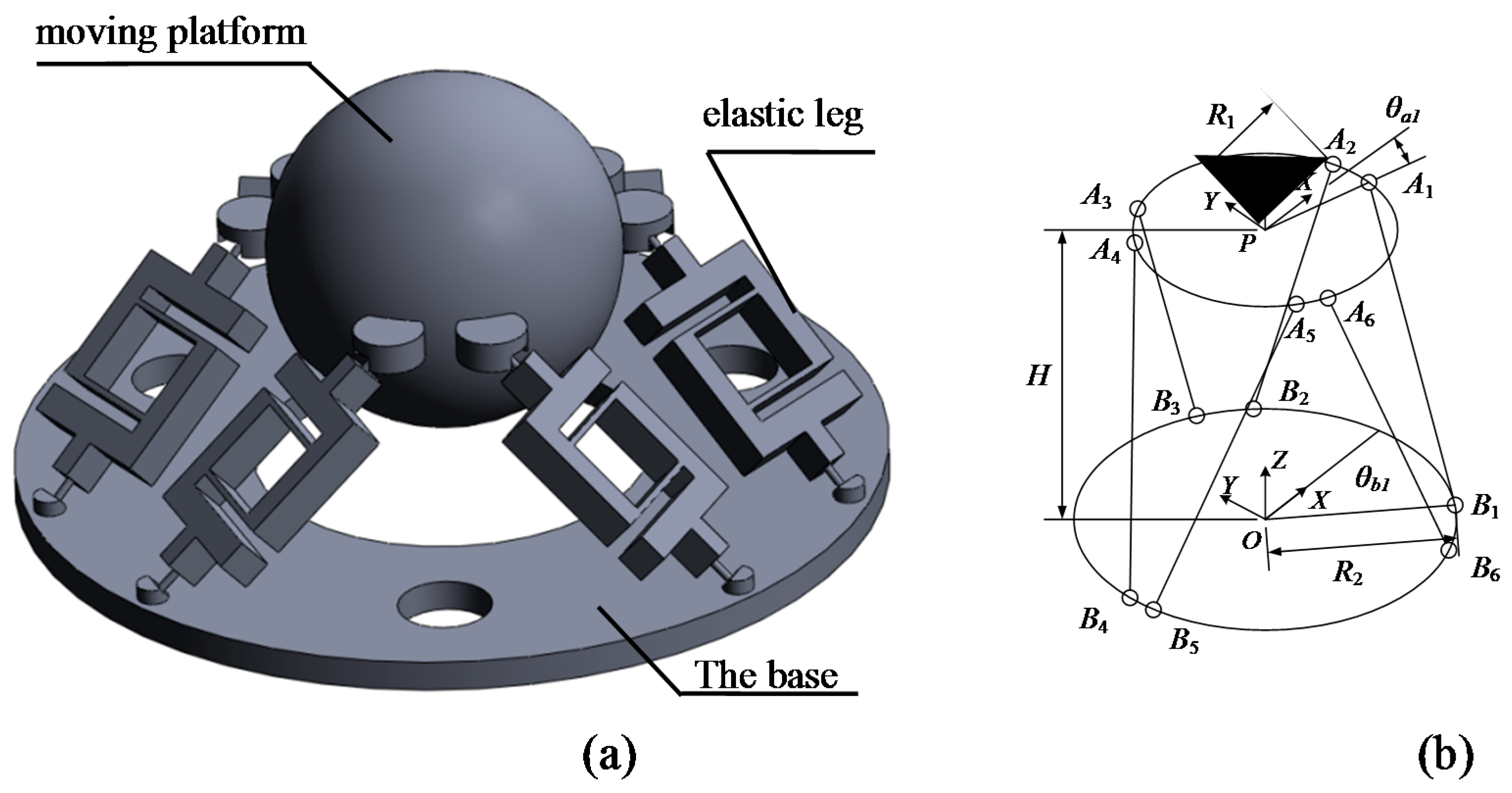
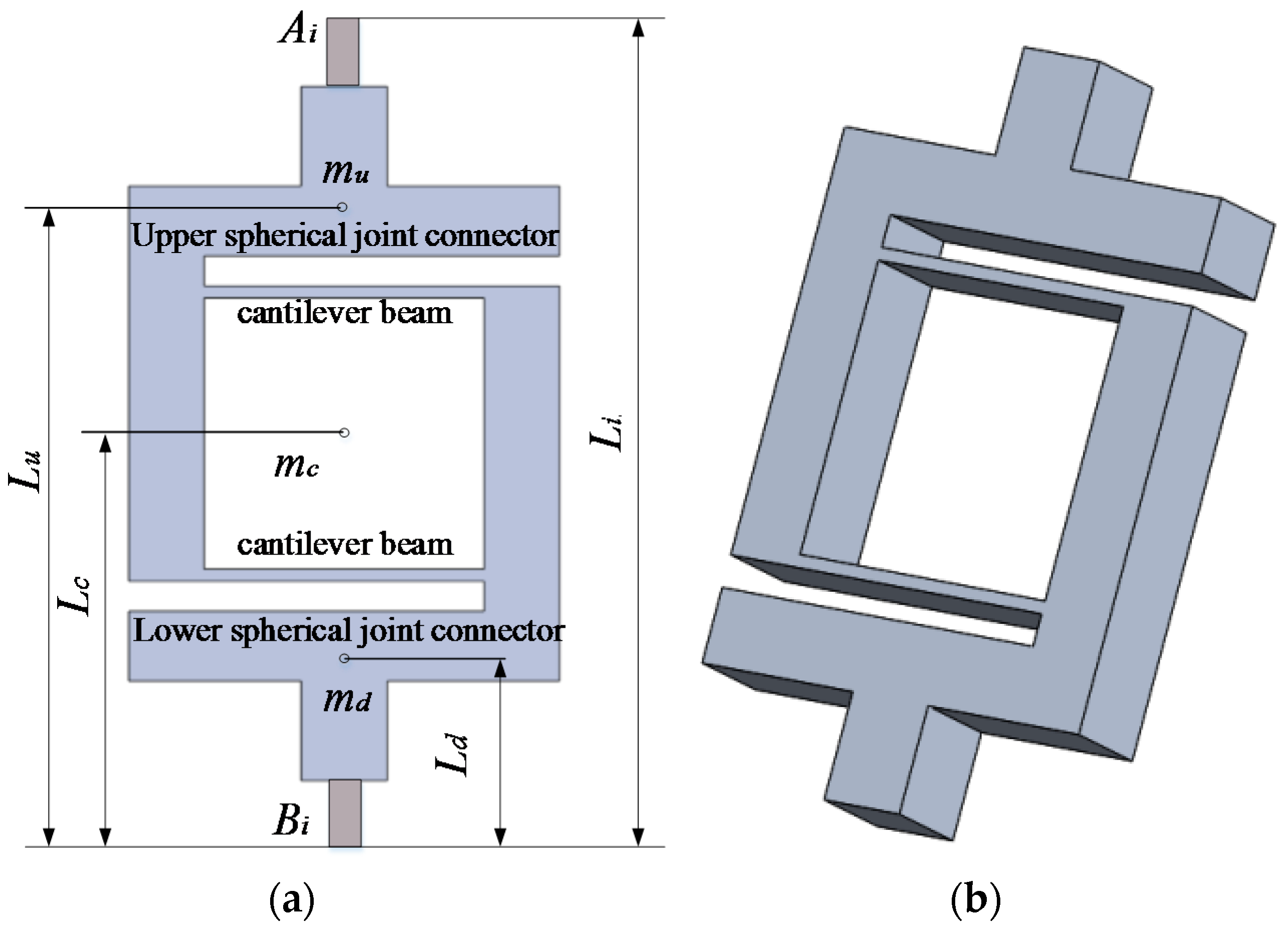
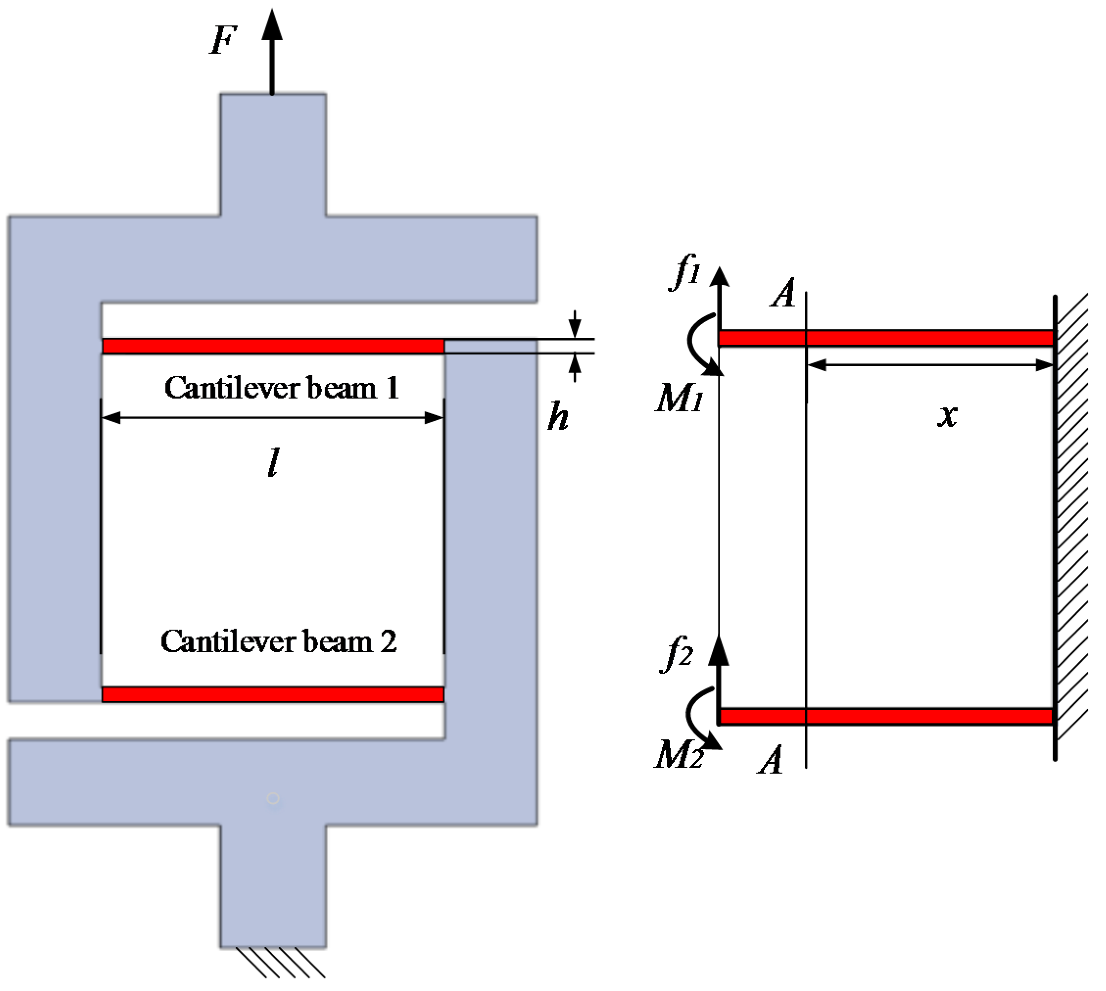
As shown in Figure 2, the DCB elastic leg consists of three parts: an upper spherical joint connector, a double cantilever beam and a lower spherical joint connector. The mass centroids of the upper spherical joint connector, double cantilever beam and lower spherical joint connector are m_u, m_c and m_d respectively. L_u, L_c and L_d denote the distance between mass centroids and the connection points B_i respectively.

The partial angular velocities on each point of the leg are identical. Substituting Equation (5) into Equation (6), the angular velocity of the leg is obtained by taking the cross product with l_i on both sides of the equation:

$${\mathit{\omega }}_l=\left[{\mathit{l}}_i\times \mathit{v}+{\mathit{l}}_i\times \left(\mathit{\omega }\times {\mathit{r}}_i\right)\right]/L_i$$

(7)

The velocity of the mass center is the vectorial sum of the axial velocity and the tangential speed along the elastic leg on the mass centroid. The axial velocity on the mass centroid of the double flexible cantilevers is half that of the whole leg, and that on the mass centroid of the lower spherical joint connector is zero. The velocity of the mass center along the elastic leg can be calculated using:

$$\{\begin{array}{l}{\mathit{U}}_u={\mathit{l}}_i\cdot \left(\mathit{v}+\mathit{\omega }\times {\mathit{r}}_i\right)\cdot {\mathit{l}}_i+{\mathit{\omega }}_l\times {\mathit{L}}_u\\ {\mathit{U}}_c=\frac{{\mathit{l}}_i\cdot \left(\mathit{v}+\mathit{\omega }\times {\mathit{r}}_i\right)\cdot {\mathit{l}}_i}{2}+{\mathit{\omega }}_l\times {\mathit{L}}_c\\ {\mathit{U}}_d={\mathit{\omega }}_l\times {\mathit{L}}_d\end{array}$$

(8)

The Lagrange equation of the accelerometer can be written as:

$$\frac{d}{dt}\left(\frac{\partial E_T}{\partial {\dot{q}}_j}\right)-\frac{\partial E_T}{\partial q_j}=Q_j$$

(9)

where E_T is the kinetic energy of the system, and q_j and ${\dot{q}}_j$ are the jth generalized coordinates and generalized speed, respectively. Q_j is the generalized force. The moving parts of the system are the six elastic legs and the moving platform, and each elastic leg consists of three moving parts. The kinetic energy of the system is a summation of the translational kinetic energy and rotational kinetic energy of the 19 moving parts, which can be expressed as:

$$E_T={\displaystyle \sum _{i=1}^{19}\frac{1}{2}\left({{\mathit{U}}_i}^T{m}_i{\mathit{U}}_i+{{\mathit{\omega }}_{li}}^T{\mathit{I}}_i{\mathit{\omega }}_{li}\right)}$$

(10)

where m_i and U_i are the mass and velocity vector of the ith part, and I_i and ω_li are the moment of inertia and angular velocity vector of the ith part, respectively. According to the differential transformation, $\frac{d}{dt}\left(\frac{\partial E_T}{\partial {\dot{q}}_j}\right)$, $\frac{\partial E_T}{\partial q_j}$ and Q_j can be calculated as:

$$\{\begin{array}{l}\frac{\partial E_T}{\partial {\dot{q}}_j}={\displaystyle \sum _{i=1}^{19}\frac{1}{2}\left(\frac{\partial {{\mathit{U}}_i}^T}{\partial {\dot{q}}_j}{m}_i{\mathit{U}}_i+{{\mathit{U}}_i}^T{m}_i\frac{\partial {\mathit{U}}_i}{\partial {\dot{q}}_j}+\frac{\partial {{\mathit{\omega }}_{li}}^T}{\partial {\dot{q}}_j}{\mathit{I}}_i{\mathit{\omega }}_{li}+{{\mathit{\omega }}_{li}}^T{\mathit{I}}_i\frac{\partial {\mathit{\omega }}_{li}}{\partial {\dot{q}}_j}\right)}\\ \frac{d}{dt}\left(\frac{\partial E_T}{\partial {\dot{q}}_j}\right)={\displaystyle \sum _{i=1}^{19}\left(\frac{\partial {{\mathit{U}}_i}^T}{\partial {\dot{q}}_j}{m}_i\frac{\partial {\mathit{U}}_i}{\partial {\dot{q}}_j}+\frac{\partial {{\mathit{\omega }}_{li}}^T}{\partial {\dot{q}}_j}{\mathit{I}}_i\frac{\partial {\mathit{\omega }}_{li}}{\partial {\dot{q}}_j}\right)}\cdot {\ddot{q}}_j\\ \frac{\partial E_T}{\partial q_j}={\displaystyle \sum _{i=1}^{19}\frac{1}{2}\left(\frac{\partial {{\mathit{U}}_i}^T}{\partial q_j}{m}_i{\mathit{U}}_i+{{\mathit{U}}_i}^T{m}_i\frac{\partial {\mathit{U}}_i}{\partial q_j}+\frac{\partial {{\mathit{\omega }}_{li}}^T}{\partial q_j}{\mathit{I}}_i{\mathit{\omega }}_{li}+{{\mathit{\omega }}_{li}}^T{\mathit{I}}_i\frac{\partial {\mathit{\omega }}_{li}}{\partial q_j}\right)}\\ Q_j={\displaystyle \sum _{i=1}^{19}\frac{\partial {{\mathit{U}}_i}^T}{\partial q_j}}\cdot m_i\mathit{g}+{\displaystyle \sum _{l=1}^6\frac{\partial {{\mathit{U}}_l}^T}{\partial q_j}}{\mathit{F}}_l\end{array}$$

(11)

where g is the gravity vector and F_l is the force of the lth elastic leg. Considering all six generalized coordinates, Lagrange equations of all the generalized coordinates are translated into differential equations for the motion:

$$\mathit{{\rm M}}\ddot{q}+\mathit{C}\dot{q}+\mathit{K}q=\mathit{F}$$

(12)

where M is the mass matrix, C is the damping matrix, K is the stiffness matrix and F is the force vector acting on the system. Because of the minimal speed on the elastic leg, the damping matrix that is related to U_i and ω_li can be ignored in the motion differential equation, which may then be simplified to:

$$\mathit{M}\ddot{\mathit{q}}\mathbf{+}\mathit{K}\mathit{q}\mathbf{=}\mathit{0}$$

(13)

3.2. Mass Matrix of the System

Referring to Equation (11), the mass matrix can be calculated as:

$$\mathit{M}={\displaystyle \sum _{i=1}^{19}({\mathit{U}}_{i,\dot{q}}^T}{m}_i{\mathit{U}}_{i,\dot{q}}+{\mathit{\omega }}_{li,\dot{q}}^T{\mathit{I}}_i{\mathit{\omega }}_{li,\dot{q}})$$

(14)

where ${\mathit{U}}_{i,\dot{q}}$ is the velocity Jacobian matrix of the ith part, derived from the velocity vector on the mass centroid with respect to the generalized speed, and ${\mathit{\omega }}_{li,\dot{q}}$ is the angular velocity matrix of the ith part, derived from the angular velocity vector of each part with respect to the generalized speed.

The mass of the moving platform can be calculated using the sphere quality function $m=\frac{4}{3}\pi r^3\rho$, where m is the quality of the sphere, r is the radius of the moving platform and ρ is the density of the material. The moment of inertia along the x-, y-, and z-axes is given by $I_x=I_y=I_z=\frac{2}{5}m{r}^2$.

The mass and moment of inertia of the elastic leg is obtained through the Solidworks environment. Based on the parallel axis theorem, the moment of inertia of the parts with respect to the base coordinate can be expressed as:

$${\mathit{I}}_i={\mathit{T}}_i{\mathit{I}}_{io}{\mathit{T}}_i^T+m_{i}diag(d_x^2,d_y^2,d_z^2)$$

(15)

where I_io is the moment of inertia with respect to the mass center; d_x, d_y and d_z are the distances between the mass center of each part and point O along the X, Y, Z axis, respectively; T_i is the rotation matrix which rotates the local coordinate system on the lower spherical joint connector to the base coordinate system; and m_i is the mass of the ith part.

The velocity Jacobian matrix and angular velocity matrix of the moving platform are formed by differentiating Equation (1) with respect to $\mathit{q}$ and $\dot{\mathit{q}}$, respectively:

$${\mathit{U}}_{m,\dot{q}}=\left[\begin{array}{cc}{\mathit{I}}_3& {\mathit{0}}_{3\times 3}\end{array}\right]$$

(16)

$${\mathit{\omega }}_{m,\dot{q}}=\left[\begin{array}{cc}{\mathit{0}}_{3\times 3}& {\mathit{I}}_{3\times 3}\end{array}\right]$$

(17)

By differentiating Equation (7) with respect to $\dot{\mathit{q}}$, the angular velocity matrix of the elastic leg is obtained:

$${\mathit{\omega }}_{l,\dot{q}}=\left[\begin{array}{cc}{\widehat{\mathit{l}}}_i& -{\widehat{\mathit{l}}}_i{\widehat{\mathit{r}}}_i\end{array}\right]/L_i$$

(18)

where the matrix marked by “^” is an anti-symmetric matrix of the vector, such as $\widehat{\mathit{u}}=\left[\begin{array}{ccc}0& -u_z& u_y\\ u_z& 0& -u_x\\ u_y& u_x& 0\end{array}\right]$, where $\mathit{u}\times \mathit{c}$ can be expressed as $\widehat{\mathit{u}}\cdot \mathit{c}$.

Differentiating Equation (8) with respect to $\dot{\mathit{q}}$, the velocity Jacobian matrix of the mass center along the elastic leg is obtained:

$$\{\begin{array}{l}{\mathit{U}}_{u,\dot{q}}=\left[\begin{array}{cc}{\mathit{l}}_i\cdot {{\mathit{l}}_i}^T+\frac{L_u}{L_i}{\widehat{\mathit{l}}}_{\mathit{i}}{\widehat{\mathit{l}}}_{\mathit{i}}& -{\mathit{l}}_i\cdot {{\mathit{l}}_i}^T\cdot {\widehat{\mathit{r}}}_i+\frac{L_u}{L_i}{\widehat{\mathit{l}}}_i\widehat{\mathit{l}}{\widehat{\mathit{r}}}_{\mathit{i}}\end{array}\right]\\ {\mathit{U}}_{c,\dot{q}}=\left[\begin{array}{cc}\frac{{\mathit{l}}_i\cdot {{\mathit{l}}_i}^T}{2}+\frac{L_c}{L_i}{\widehat{\mathit{l}}}_{\mathit{i}}{\widehat{\mathit{l}}}_{\mathit{i}}& \frac{-{\mathit{l}}_i\cdot {{\mathit{l}}_i}^T\cdot {\widehat{\mathit{r}}}_i}{2}+\frac{L_c}{L_i}{\widehat{\mathit{l}}}_i\widehat{\mathit{l}}{\widehat{\mathit{r}}}_{\mathit{i}}\end{array}\right]\\ {\mathit{U}}_{d,\dot{q}}=\left[\begin{array}{cc}\frac{L_d}{L_i}{\widehat{\mathit{l}}}_i{\widehat{\mathit{l}}}_i& \frac{L_d}{L_i}{\widehat{\mathit{l}}}_i{\widehat{\mathit{l}}}_i{\widehat{\mathit{r}}}_i\end{array}\right]\end{array}$$

(19)

3.3. Stiffness Matrix of the System

Referring to Equations (2) and (3), the unit line vectors of the elastic legs can be calculated as

$${\mathit{l}}_i=\left[\begin{array}{c}{\mathit{s}}_i\\ {\mathit{s}}_{ri}\end{array}\right]$$

(20)

where ${\mathit{s}}_i=\left({\mathit{A}}_i-{\mathit{B}}_i\right)/\left|{\mathit{A}}_i-{\mathit{B}}_i\right|$, ${\mathit{s}}_{ri}=\mathit{r}\times \mathit{s}=\left({\mathit{A}}_i\times \left({\mathit{A}}_i-{\mathit{B}}_i\right)\right)/\left|{\mathit{A}}_i-{\mathit{B}}_i\right|=\left({\mathit{B}}_i\times {\mathit{A}}_i\right)/\left|{\mathit{A}}_i-{\mathit{B}}_i\right|$.

For the six-axis accelerometer system, the force Jacobian matrix can be obtained:

$$\mathit{J}={\left[\begin{array}{llllll}{\mathit{l}}_1& {\mathit{l}}_2& {\mathit{l}}_3& {\mathit{l}}_4& {\mathit{l}}_5& {\mathit{l}}_6\end{array}\right]}^T$$

(21)

Based on the CCT, the stiffness matrix of the system is expressed as:

$$\mathit{K}={\mathit{J}}^T{\mathit{K}}_l\mathit{J}$$

(22)

where K_l is the diagonal stiffness matrix of the elastic legs, which can be written as:

$${\mathit{K}}_l=diag\left(k_1,k_2,k_3,k_4,k_5,k_6\right)$$

(23)

According to [2], the elastic leg force matrix can be calculated as:

$${\mathit{F}}_l={\mathit{K}}_l\mathit{J}\mathit{q}={\left({\mathit{J}}^T\right)}^{-1}\left(-\mathit{M}\ddot{\mathit{q}}\right)$$

(24)

4. Analysis of the DCB Elastic Element

4.1. Structure of the Elastic Legs

DCB structure is an elastic-sensitive element. Compared with the single cantilever beam, DCB structure performs better elasticity and stability characteristics, and the strain value is also enhanced. In this accelerometer, the DCB structure is applied as the elastic element. With a high strain of the DCB, the sensitivity of the system and the accuracy of the sensor are improved.

Figure 3 shows the force analysis of the DCB elastic leg, F is assumed to be a lift force on the top of the leg, and the end of the leg is fixed. The upper and lower spherical joint connectors are assumed to be rigid. The equivalent effect on the first cantilever beam is a combination of the force f₁ and moment M₁, and that on the second beam is f₂ and M₂. According to the principle of balanced forces and moments, the force equation of the DCB leg can be calculated as:

$$\{\begin{array}{c}{f}_1=f_2=\frac{F}{2}\\ M_1=M_2=\frac{Fl}{4}\end{array}$$

(25)

where l is length of the cantilever beam. In Figure 4, A-A is an arbitrary cross section of the cantilever beam. Based on the differential equation of the deflection, the deflection of the section A-A is obtained:

$$\{\begin{array}{c}{w}_f=\frac{F{l}^2\left(3l-x\right)}{12EI}\\ w_M=\frac{M_1{x}^2}{2EI}=\frac{Fl{x}^2}{8EI}\end{array}$$

(26)

where I is the moment of inertia of the cantilever beam, w_f is the deformation of the cross section A-A caused by the force F, w_M is the deformation caused by the moment M₁ and x is the distance between the section A-A and the fixed port of the cantilever beam. Based on the moment of inertia of a rectangular section, the moment of inertia I can be expressed as:

$$I=\frac{b\cdot h^3}{12}$$

(27)

where h is the width and b denotes thickness. Force analysis proves that force F and moment M have an opposite effect on the deflection. Total deflection is expressed as $w=w_f-w_M$. The total deflection of section A-A is expressed as:

$$w_{A-A}=\frac{F\left(3l{x}^2-2x^3\right)}{24EI}=\frac{F\left(3l{x}^2-2x^3\right)}{2Eb{h}^3}$$

(28)

The maximum deformation of the beam is obtained when the distance between the section A-A and the fixed port equals the length of the beam. Referring to the Equations (27) and (28), the equivalent stiffness coefficient of the DCB leg can be obtained as:

$$k_l=2\cdot \frac{F}{w}=\frac{24EI}{l^3}=\frac{2Eb{h}^3}{l^3}$$

(29)

4.2. Numerical Calculation

Parameters of the elastic legs are determined by the strength of the DCB structure, size of the accelerometer and the manufacturing costs. Maximum moment is at the mode point of the beam, which can be calculated as:

$$M_{\text{max}}=\frac{F_i}{2}\cdot l-\frac{F_i}{4}\cdot l=\frac{F_i\cdot l}{4}$$

(30)

where F_i is the force loading on the ith elastic leg, and M_max is the maximum moment on the beam. Based on the formula for the normal stress of the beam, the maximum bending stress of the DCB can be calculated as

$${\sigma }_{\text{max}}=\frac{M_{\text{max}}\cdot h}{2I}$$

(31)

where σ_max is the maximum bending stress of the DCB. After analyzing the isotropic of the accelerometer and considering the manufacturing costs, the improved parameters of the accelerometer and the elastic legs and angle parameters of the accelerometer are obtained as shown in

Table 1. Parameters of the six-axis accelerometer.

Parameter	Value (mm)
RA	25
RB	52
r	22.5
H	30
b	5
h	0.6
l	13

and

Table 2. Angle parameters of the six-axis accelerometer.

Sequence Number	θai	θbi
i = 1	−π/12	−π/4
i = 2	π/12	π/4
i = 3	7π/12	5π/12
i = 4	3π/4	11π/12
i = 5	5π/4	13π/12
i = 6	17π/12	19π/12

[33].

Based on the stress requirements and the cost of component processing, the elastic element material is an aluminum alloy with elastic modulus E = 6.9E10 Pa. Substituting the parameters in Table 1 and Table 2 into Equation (21), the Jacobian matrix of the accelerometer can be calculated as:

$$\mathit{J}=\left[\begin{array}{cccccc}-0.2882& -0.2882& -0.4550& 0.7432& 0.7432& -0.4550\\ 0.6918& -0.6918& -0.5955& 0.0963& 0.0963& 0.5955\\ -0.6621& -0.6621& -0.6621& -0.6621& -0.6621& -0.6621\\ 0.0043& -0.0043& -0.0160& -0.0117& 0.0117& 0.0160\\ 0.0160& 0.0160& -0.0043& -0.0117& -0.0117& -0.0043\\ 0.0148& -0.0148& 0.0148& -0.0148& 0.0148& -0.0148\end{array}\right]$$

(32)

Substituting the parameters in Table 1 and Table 2 into Equation (20), the mass matrix can be calculated as:

$$\mathit{M}=\left[\begin{array}{cccccc}0.4425& 0& -0.0001& 0& 0& 0\\ 0& 0.4404& 0& 0& 0& 0\\ -0.0001& 0& 0.4459& 0& 0& 0\\ 0& 0& 0& 0.0001& 0& 0\\ 0& 0& 0& 0& 0.0001& 0\\ 0& 0& 0& 0& 0& 0.0001\end{array}\right]$$

(33)

Substituting the parameters in Table 1 and Table 2 into Equation (22), the stiffness matrix can be calculated as:

$$\mathit{K}={10}^5\cdot \left[\begin{array}{cccccc}1.1429& 0& 0& 0& -0.0154& 0\\ 0& 1.1429& 0& 0.0154& 0& 0\\ 0& 0& 1.7844& 0& 0& 0\\ 0& 0.0154& 0& 0.0006& 0& 0\\ -0.0154& 0& 0& 0& 0.0006& 0\\ 0& 0& 0& 0& 0& 0.0009\end{array}\right]$$

(34)

To analyze the sensitivity of the accelerometer, acceleration components ${\mathit{g}}_x={\left[\begin{array}{cccccc}9.8& 0& 0& 0& 0& 0\end{array}\right]}^{\mathrm{T}}$, ${\mathit{g}}_y={\left[\begin{array}{cccccc}0& 9.8& 0& 0& 0& 0\end{array}\right]}^{\mathrm{T}}$ and ${\mathit{g}}_z={\left[\begin{array}{cccccc}0& 0& 9.8& 0& 0& 0\end{array}\right]}^{\mathrm{T}}$ are loaded onto the moving platform for deformation analysis. Substituting Equations (32)–(34) into Equation (24), the forces of the legs are calculated as:

$$\{\begin{array}{c}{F}_x={\left[\begin{array}{cccccc}0.6048& 0.6048& -2.2572& 1.6524& 1.6524& -2.2572\end{array}\right]}^{\mathrm{T}}\\ F_y={\left[\begin{array}{cccccc}2.2572& -2.2572& -0.6048& 1.6524& -1.6524& 0.6048\end{array}\right]}^{\mathrm{T}}\\ F_z={\left[\begin{array}{cccccc}-1.0475& -1.0475& -1.0475& -1.0475& -1.0475& -1.0475\end{array}\right]}^{\mathrm{T}}\end{array}$$

(35)

where F_x is the force matrix of the legs when acceleration g_x is loaded onto the moving platform, F_y is the force matrix of the legs when acceleration g_y is loaded on the moving platform, and F_z is the force matrix of the legs when acceleration g_z is loaded on the moving platform. A positive number indicates a tensional force, and a negative number indicates a compressional force.

Referring to Equation (28), the distance between the section A-A and the fixed port is set as the variable, and the deformation curves of the six beams are shown in Figure 4.

To validate the theoretical model, a finite element method was applied to the model and strain analysis of the system.

As shown in Figure 5, The finite element model was established in the ANSYS Workbench environment. The accelerometer was meshed using hexahedral elements, and the material of the moving platform was a copper alloy. The elastic modulus was 1.17E11 Pa, Poisson’s ratio was 0.31, and the density was 8900 kg/m³. The material of the elastic element was an aluminum alloy, with elastic modulus of 6.9E10 Pa, Poisson’s ratio of 0.3 and density of 2700 kg/m³. The base is fixed before running the model.

Accelerations g_x, g_y and g_z are loaded onto the moving platform in the strain analysis. Comparing the theoretical deflection with that of the simulations, an overall trend is apparent. The maximum theoretical deflections are 3.33 × 10⁻² mm along the x-axis, 3.33 × 10⁻² mm along the y-axis and 1.54 × 10⁻² mm along the z-axis. The maximum simulated deflections are 3.74 × 10⁻² mm along the x-axis, 3.77 × 10⁻² mm along the y-axis and 1.76 × 10⁻² mm along the z-axis. The coincidence rate reaches 89.0% along the x-axis, 88.3% along the y-axis and 87.5% along the z-axis.

5. Theoretical Analysis of the Elastic Leg Strain

There are four sensing elements positioned at predetermined locations on the elastic leg. Figure 6 depicts the location of the strain gauges; the Wheatstone bridge arrangement for a single element is also shown. Each bridge is excited by a stable 5-V power supply. The resistances of the strain gauges are equal initially and can be described as:

$$R_1=R_2=R_3=R_4=R$$

(36)

When the accelerometer is in a working state, the resistances of the strain gauges change by an amount given by ΔR₁, ΔR₂, ΔR₃, and ΔR₄. In the case where ΔR _i << R(i = 1,2,3,4), the output voltage can be simplified to:

$$\Delta U_{BD}=\frac{U}{4}(\frac{\Delta R_1}{R}-\frac{\Delta R_2}{R}+\frac{\Delta R_3}{R}-\frac{\Delta R_4}{R})=\frac{U}{4}K({\epsilon }_1-{\epsilon }_2+{\epsilon }_3-{\epsilon }_4)$$

(37)

where K is the sensitivity coefficient of the strain gauge and ε_i(i = 1,2,3,4)is the strain value of each strain gauge. ${\epsilon }_1$ and ${\epsilon }_3$ are opposite in sign to ${\epsilon }_2$ and ${\epsilon }_4$, and U is the power supplied to the system. By making use of the integral, strain ${\epsilon }_1$ and ${\epsilon }_3$ are calculated using:

$${\epsilon }_1=\frac{2{\displaystyle {\int }_0^{\frac{l}{2}}{\epsilon }_{x}dx}}{l},{\epsilon }_2=\frac{2{\displaystyle {\int }_{\frac{l}{2}}^l{\epsilon }_{x}dx}}{l},{\epsilon }_3=-\frac{2{\displaystyle {\int }_{\frac{l}{2}}^l{\epsilon }_{x}dx}}{l},{\epsilon }_4=-\frac{2{\displaystyle {\int }_0^{\frac{l}{2}}{\epsilon }_{x}dx}}{l}$$

(38)

where ${\epsilon }_x=\frac{h{M}_x}{2IE}$ is the strain of the beam on section A-A and M_x is the bending moment on section A-A, which can be calculated as $M_x=\frac{F\left(l-2x\right)}{4}$. The strain of the beam can be expressed as:

$$\{\begin{array}{c}{\epsilon }_1={\epsilon }_3=\frac{3Fl}{4Eb{h}^2}\\ {\epsilon }_2={\epsilon }_4=-\frac{3Fl}{4Eb{h}^2}\end{array}$$

(39)

Referring to Equation (39), the strain of one strain gauge in the elastic element is 8.22 × 10⁻² mm with the accelerometer a_z = 1 g. Compared with the reference 20 (With acceleration a_z = 1 g, maximal positive strain of the accelerometer is 6.903 × 10⁻⁵ mm), DCB structure shows better strain performance. Measurement of the strain gauge shows that the sensitivity coefficient K is 4. The output voltage can be expressed as:

$$\Delta U_{BD}=\frac{3UKFl}{4Eb{h}^2}$$

(40)

Sensitivities of the accelerometer means the output voltage of each elastic leg in the unit acceleration. Referring to Equations (24) and (40), the ratio of the output voltage to the acceleration can be calculated. Theoretical sensitivities of the accelerometer along the x-axis, y-axis and z-axis were obtained as:

$$\{\begin{array}{c}\Delta {{\mathit{U}}_x}^{\prime }=\left[\begin{array}{cccccc}0.0969& 0.0969& 0.3616& 0.2647& 0.2647& 0.3616\end{array}\right]\\ \Delta {{\mathit{U}}_y}^{\prime }=\left[\begin{array}{cccccc}0.3616& 0.3616& 0.0969& 0.2647& 0.2647& 0.0969\end{array}\right]\\ \Delta {{\mathit{U}}_z}^{\prime }=\left[\begin{array}{cccccc}0.1678& 0.1678& 0.1678& 0.1678& 0.1678& 0.1678\end{array}\right]\end{array}$$

(41)

where ΔU_x’, ΔU_y’ and ΔU_z’ are the theoretical sensitivity matrixes of the elastic legs along the x-, y- and z-axes, respectively, in units of mV/(m/s²).

6. Sensitivity Experiments

In order to verify the sensitivity of the accelerometer, a calibration test on the linear sensitivity of the accelerometer was conducted (certificate number: LSzb2011-0416). As shown in Figure 7, the test system consisted of five parts: an accelerometer, multi-channel dynamic strain gauge, data acquisition system, data processing system and calibration platform. Strain gauges are located on the accelerometer and Wheatstone bridge circuit is applied in the system. The multi-channel dynamic strain gauge can achieve calibration of 12 channels simultaneously and transfer the analog signals into digital signals to a computer. The data acquisition system was connected to a microcomputer data processing system through a USB interface. The frequency of vibration standard device APS 129 ELECTRO-SEIS is applied to the calibration platform.

A calibration test on the linear sensitivity of the accelerometer was conducted. As shown in Figure 7, the test system consisted of five parts: an accelerometer, multi-channel dynamic strain gauge, data acquisition system, data processing system and calibration platform. The multi-channel dynamic strain gauge can achieve calibration of 12 channels simultaneously and transfer this information to a computer. The data acquisition system was connected to a microcomputer data processing system through a USB interface.

The system requires preheating for 30 min during the process of demarcation and calibration. The acceleration load g_z was divided into 10 equal points along the z-axis. Loading was sinusoidal with a reference frequency of 16 Hz. Output voltages of the elastic legs, magnified 1000-fold, are shown in

Table 3. Output voltage of each channel on z-axis acceleration.

No.	Acceleration (m/s2)	Output Voltage (mv)
		Leg 1	Leg 2	Leg 3	Leg 4	Leg 5	Leg 6
1	1	132.4	143.8	116	128.2	137.8	131.6
2	2	277.8	289.2	232.4	258.8	274	262.8
3	3	414	434.4	348.3	387	412.5	394.5
4	4	554	578.4	465.2	519.6	552.4	526.8
5	5	690	721	581.5	646	688	660
6	6	837	867.6	696.6	777	824.4	796.2
7	7	970.2	1012.2	814.8	906.5	964.6	928.9
8	8	1110.4	1155.2	932	1036	1098.4	1060.8
9	9	1249.2	1298.7	1046.7	1163.7	1237.5	1198.8
10	10	1389	1442	1165	1292	1376	1331

. The sensitivity shows a strong linear relationship, which can be calculated as:

Acceleration test loads along the x and y-axis were 1 m/s², divided into 10 equal points. Output voltages of the elastic legs, magnified 1000-fold, are shown in

Table 4. Output voltage of each channel on x-axis acceleration.

No.	Acceleration (m/s2)	Output Voltage (mv)
		Leg 1	Leg 2	Leg 3	Leg 4	Leg 5	Leg 6
1	0.1	8.41	9.43	40.03	34.51	37.29	41.92
2	0.2	17.06	18.9	80.24	69.18	74.54	83.46
3	0.3	25.68	28.62	120.72	103.11	111.87	125.01
4	0.4	34.16	38.04	160.8	137.72	148.72	166.28
5	0.5	42.1	47.8	200.8	172	185.5	207.5
6	0.6	50.04	58.26	241.08	206.46	221.7	249.06
7	0.7	56.49	69.16	281.54	240.66	258.79	290.08
8	0.8	65.68	78	321.28	275.28	294.32	331.6
9	0.9	73.35	87.93	361.62	309.42	331.38	372.78
10	1	80.4	98.6	401.3	343.5	367.4	414.3

and

Table 5. Output voltage of each channel on y-axis acceleration.

No.	Acceleration (m/s2)	Output Voltage (mv)
		Leg 1	Leg 2	Leg 3	Leg 4	Leg 5	Leg 6
1	0.1	47.22	47.43	17.28	27.47	34.79	14.49
2	0.2	94.44	94.68	34.9	55.3	69.48	28.96
3	0.3	142.08	142.5	51.66	82.35	103.56	43.62
4	0.4	189.48	188.68	69.4	109.28	138.04	58.2
5	0.5	236.55	236.15	86.7	136.55	172.1	72.85
6	0.6	283.8	284.04	103.92	163.74	206.4	87.36
7	0.7	331.38	330.68	121.52	190.26	240.66	101.92
8	0.8	378.64	377.76	138.8	217.52	275.04	116.56
9	0.9	425.61	424.53	156.42	244.26	308.88	131.04
10	1	472.8	472.2	173.8	271.2	342.9	145.6

.

The result of the output voltage shows a strong linear relationship. Based on the arithmetic mean summation method, the sensitivity of the accelerometer can be calculated as:

$$\{\begin{array}{l}\Delta {\mathit{U}}_z=\frac{1}{10}{\displaystyle \sum _{i=1}^{10}\frac{{\mathit{U}}_{zi}}{a_{zi}}}=\left[\begin{array}{cccccc}0.138& 0.144& 0.116& 0.129& 0.137& 0.132\end{array}\right]\\ \Delta {\mathit{U}}_x=\frac{1}{10}{\displaystyle \sum _{i=1}^{10}\frac{{\mathit{U}}_{xi}}{a_{xi}}}=\left[\begin{array}{cccccc}0.083& 0.096& 0.402& 0.344& 0.370& 0.416\end{array}\right]\\ \Delta {\mathit{U}}_y=\frac{1}{10}{\displaystyle \sum _{i=1}^{10}\frac{{\mathit{U}}_{yi}}{a_{yi}}}=\left[\begin{array}{cccccc}0.473& 0.473& 0.173& 0.273& 0.344& 0.145\end{array}\right]\end{array}$$

(42)

where ΔU_z, ΔU_x, and ΔU_y are the sensitivity matrix of the elastic legs along the z-, x- and y-axis, in units of V/m/s²; U_zi, U_xi, and U_yi are the output voltage matrix of the elastic legs in the ith experiment; and a_zi, a_xi, and a_yi are the acceleration loaded on the system in the ith experiment, respectively.

To verify the theoretical model, theoretical result magnified 1000-fold is compared with that of the experiment. Based on the arithmetic mean summation method, theoretical sensitivity accuracies along the x-, y- and z-axes of 90.4%, 74.9% and 78.9% with respect to the test data are obtained.

Acceleration loading times of the experiments is set as n = 10. Based on the arithmetic mean summation method, the measurement precision of the accelerometer is obtained in

Table 6. Measurement precision of the six-axis accelerometer.

Acceleration (m/s2)	ax Error (%) n = 10	ay Error (%) n = 10	Acceleration (m/s2)	az Error (%) n = 10
0.1	2.6	0.6	1	1.31
0.2	2.55	0.5	2	1.22
0.3	2.5	0.57	3	1.1
0.4	2.45	0.53	4	1.11
0.5	2.36	0.52	5	1.23
0.6	2.45	0.52	6	1.16
0.7	2.47	0.5	7	1.02
0.8	2.48	0.5	8	1.11
0.9	2.48	0.53	9	1.15
1	2.44	0.52	10	1.11
Max Error (%)	2.6	0.6		1.31

.

As can be seen in Table 6, the maximum errors of a_x, a_y and a_z are 2.6%, 0.6% and 1.31% respectively.

Table 7. Measurement precision of another parallel type six-axis accelerometer.

Acceleration (m/s2)	ax Error (%)	ay Error (%)	az Error (%)
0.15 g	5.058	7.428	\
0.30 g	\	\	6.017
1.38 g	6.899	\	7.470
2.75 g	\	6.99	\
3.82 g	\	7.108	5.984
7.64 g	7.479	\	\
Min Error (%)	5.058	6.99	5.984

shows the measurement precision of another accelerometer with parallel structure [34]. The minimum error of a_x, a_y and a_z are 5.058%, 6.99% and 5.984% respectively. Compared with the data in Table 7, the experiments data in Table 6 prove that accelerometer with DCB elastic element performs a great sensitive and precision characteristics.

7. Conclusions

A theoretical model of a six-axis accelerometer with a DCB elastic element is presented based on a parallel mechanism. FEA simulations and prototype experiments prove that the accelerometer shows high sensitivity performance. The main conclusions are:

• In this paper, a dynamics model for the accelerometer is established based on the Lagrange equation, and the mass and stiffness matrices obtained. Based on structural mechanics, characteristics of the DCB elastic element are obtained. A theoretical model of the whole accelerometer is calculated.
• Accelerations g_x, g_y and g_z are loaded onto the moving platform, and the deformation of the elastic legs calculated. By comparison with the FEA simulation, the coincidence rate of the deformation reached 89.0% along the x-axis, 88.3% along the y-axis and 87.5% along the z-axis.
• The prototype experiments show that the six-axis accelerometer with the DCB elastic element is highly sensitive. Compared to theoretical sensitivities, the accuracy of the x-, y- and z-axes measurements was found to be 84.6%, 75.1% and 79.8%, respectively. Prototype experiments prove the reliability of the theoretical model. The measurement errors of linear accelerations ax, ay and az are 2.6%, 0.6% and 1.31%, respectively.
• Because of the limited equipment, only linear acceleration can be loaded in the accelerometer calibration experiment. The analysis and results of the experiments are for the three linear directions only.

References

1. Wang, Z.; Li, Z.; He, J.; Yao, J.; Zhao, Y. Optimal design and experiment research of a fully pre-stressed six-axis force/torque sensor. Measurement 2013, 46, 2013–2021. [Google Scholar] [CrossRef]
2. Yao, J.T.; Li, L.J.; Xu, Y.D.; Zhao, Y.S. Statically determinate measurement model and calibration method of statically indeterminate six-axis force sensor. Chin. J. Sci. Instrum. 2013, 34, 1927–1933. [Google Scholar]
3. You, J.J.; Li, C.G.; Wu, H.T. Research on Hamiltonian Dynamics of Parallel Type Six-axis Accelerometer. J. Mech. Eng. 2012, 48, 9–17. [Google Scholar] [CrossRef]
4. Yu, C.Z.; Zhang, X.Y.; Jia, Q.X.; Li, J. Theoretical research on a six-axis accelerometer for humanoid robot wrist. Chin. J. Sci. Instrum. 2011, 32, 1903–1909. [Google Scholar]
5. Wu, L.C.; Nangia, V.; Bui, K.; Hammoor, B.; Kurt, M.; Hernandez, F.; Kuo, C.; Camarillo, D.B. In vivo evaluation of wearable head impact sensors. Ann. Biomed. Eng. 2016, 44, 1234–1245. [Google Scholar] [CrossRef] [PubMed]
6. Chen, H.; Kurt, M.; Lee, Y.S.; McFarland, D.M.; Bergman, L.A.; Vakakis, A.F. Experimental system identification of the dynamics of a vibro-impact beam with a view towards structural health monitoring and damage detection. Mech. Syst. Signal Process. 2014, 46, 91–113. [Google Scholar] [CrossRef]
7. Liu, S.A.; Tzo, H.L. A novel six-component force sensor of good measurement isotropy and sensitivities. Sens. Actuators A Phys. 2002, 100, 223–230. [Google Scholar] [CrossRef]
8. Stewart, D. A platform with six degrees of freedom. Proc. Inst. Mech. Eng. 1965, 180, 371–386. [Google Scholar] [CrossRef]
9. Sorli, M.; Zhmud, N. Investigation of force and moment measurement system for a robotic assembly hand. Sens. Actuators A Phys. 1993, 37, 651–657. [Google Scholar] [CrossRef]
10. Wang, H.R.; Chen, G.L.; Gao, F.; Huang, Z. Design of six axis force/torque sensor based on Stewart Platform related to isotropy. Chin. J. Mech. Eng. 2000, 36, 49–52. [Google Scholar] [CrossRef]
11. Ferraresi, C.; Pastorelli, S.; Sorli, M.; Zhmud, N. Static and dynamic behavior of a high stiffness Stewart platform-based force/torque sensor. J. Robot. Syst. 1995, 12, 883–893. [Google Scholar] [CrossRef]
12. Hou, Y.L.; Zeng, D.X.; Yao, J.T.; Kang, K.J.; Lu, L.; Zhao, Y.S. Optimal design of a hyperstatic Stewart platform-based force/torque sensor with genetic algorithms. Mechatronics 2009, 19, 199–204. [Google Scholar] [CrossRef]
13. Kerr, D.R. Analysis, properties, and design of a Stewart platform transducer. J. Mech. Des. 1989, 111, 25–28. [Google Scholar] [CrossRef]
14. Dwarakanath, T.A.; Dasgupta, B.; Mruthyunjaya, T.S. Design and development of a Stewart platform-based force–torque sensor. Mechatronics 2001, 11, 793–809. [Google Scholar] [CrossRef]
15. Dwarakanath, T.A.; Bhutani, G. Beam type hexapod structure based six component force/torque sensor. Mechatronics 2011, 21, 1279–1287. [Google Scholar] [CrossRef]
16. Seibold, U.; Kübler, B.; Hirzinger, G. Prototype of Instrument for Minimally Invasive Surgery with 6-Axis Force Sensing Capability. In Proceedings of the 2005 IEEE International Conference on Robotics and Automation, Barcelona, Spain, 2005; pp. 496–501.
17. Krouglicof, N.; Alonso, L.M.; Keat, W.D. Development of a mechanically coupled, six degree-of-freedom load platform for biomechanics and sports medicine. In Proceedings of the IEEE International Conference on Systems, Man and Cybernetics, Hague, The Netherlands, 2004; pp. 4426–4431.
18. Gao, F.; Zhang, Y.; Zhao, X.C.; Guo, W.Z. The design and applications of F/T sensor based on Stewart platform. In Proceedings of the 12th IFToMM World Congress, Besancon, France, 2007.
19. Ranganath, R.; Nair, P.S.; Mruthyunjaya, T.S.; Ghosal, A. A force—Torque sensor based on a Stewart Platform in a near-singular configuration. Mech. Mach. Theory 2004, 39, 971–998. [Google Scholar] [CrossRef]
20. Gao, Z.; Zhang, D. Design, analysis and fabrication of a multidimensional acceleration sensor based on fully decoupled compliant parallel mechanism. Sens. Actuators A Phys. 2010, 163, 418–427. [Google Scholar] [CrossRef]
21. Yang, B.; Wang, X.J.; Dai, B.; Liu, X. A new z-axis resonant micro-accelerometer based on electrostatic stiffness. Sensors 2015, 15, 687–702. [Google Scholar] [CrossRef] [PubMed]
22. Zhang, J.; Su, Y.; Shi, Q.; Qiu, A.P. Microelectromechanical resonant accelerometer designed with a high sensitivity. Sensors 2015, 15, 30293–30310. [Google Scholar] [CrossRef] [PubMed]
23. Yun, Y.; Li, Y. A general dynamics and control model of a class of multi-DOF manipulators for active vibration control. Mech. Mach. Theory 2011, 46, 1549–1574. [Google Scholar] [CrossRef]
24. Yao, J.T. Basic Theoretical and Experimental Research on Large Range Parallel Six-Axis Force Sensor. Ph.D. Thesis, Yanshan University, Qin Huangdao, China, 2010. [Google Scholar]
25. You, J.J.; Li, C.G.; Wu, H.T. Study on the scheme design and modeling of six-axis accelerometer based on paral lel mechanism. J. Vib. Eng. 2012, 25, 658–666. [Google Scholar]
26. De Morais, A.B. Analysis of the metal adhesively bonded double cantilever beam specimen. Int. J. Adhes. Adhes. 2015, 8, 8–14. [Google Scholar] [CrossRef]
27. De Morais, A.B. Beam analysis of the double cantilever beam specimen with fibre bridging. J. Compos. Mater. 2014, 14, 1681–1688. [Google Scholar] [CrossRef]
28. Wang, J.H.; Jin, D.D.; Cao, S.F. Research of Strain-Measurement Sensor Based on Double Cantilever Beam. Chin. J. Sens. Actuators 2005, 18, 589–595. [Google Scholar]
29. Yu, W.J.; Xiao, X.T.; Liu, Y.; Zheng, H.J. Design and Application of Elastic-sensitive Element on Double Cantilever Beam. Instrum. Tech. Sens. 2010, 12, 9–11. [Google Scholar]
30. Kurt, M.; Eriten, M.; McFarland, D.M.; Bergman, L.A.; Vakakis, A.F. Methodology for model updating of mechanical components with local nonlinearities. J. Sound Vib. 2015, 357, 331–348. [Google Scholar] [CrossRef]
31. Kurt, M.; Eriten, M.; McFarland, D.M.; Bergman, L.A.; Vakakis, A.F. Strongly nonlinear beats in the dynamics of an elastic system with a strong local stiffness nonlinearity: Analysis and identification. J. Sound Vib. 2014, 333, 2054–2072. [Google Scholar] [CrossRef]
32. Kang, C. Closed-form force sensing of a 6-axis force transducer based on the Stewart platform. Sens. Actuators A Phys. 2001, 90, 31–37. [Google Scholar] [CrossRef]
33. Yu, C.Z.; Liu, J.H.; Sun, Z.B. Parameters optimization of a six-axis accelerometer based on parallel mechanism. Chin. J. Sci. Instrum. 2014, 35, 2216–2222. [Google Scholar]
34. You, J.J.; Li, C.G.; Wu, H.T. Parameter identification of parallel type six-axis accelerometer. Opt. Precis. Eng. 2013, 21, 2627–2638. [Google Scholar]
Figure 1. Structure of the six-axis accelerometer: (a) three-dimensional model of a small range six-axis accelerometer; and (b) theoretical model of the six-axis accelerometer.
Sensors 16 01552 g001
Figure 2. Structure of the elastic leg. (a) Front side of the elastic leg; (b) 3D model of the elastic leg.
Sensors 16 01552 g002
Figure 3. Force analysis of the double cantilever beam (DCB) elastic leg.
Sensors 16 01552 g003
Figure 4. Deformation of the six beams: (a) deformation under a load gx on the moving platform; (b) deformation under a load gy on the moving platform; and (c) deformation under a load gz on the moving platform.
Sensors 16 01552 g004
Figure 5. Deformation of the six beams in ANSYS Workbench: (a) deformation under a load gx on the moving platform in ANSYS Workbench; (b) deformation under a load gy on the moving platform in ANSYS Workbench; and (c) deformation under a load gz on the moving platform in ANSYS Workbench.
Sensors 16 01552 g005
Figure 6. The location of the strain gauges and the bridge arrangement for one element: (a) the location of the strain gauges; and (b) bridge arrangement.
Sensors 16 01552 g006
Figure 7. Calibration test for linear sensitivity of the accelerometer: (a) the calibration system for the six-axis accelerometer; and (b) prototype of the elastic element of the six-axis accelerometer.
Sensors 16 01552 g007