Article

Directly Estimating Endmembers for Compressive Hyperspectral Images

Depart of Automatic Test and Control, Harbin Institute of Technology, Harbin 150080, China
*
Author to whom correspondence should be addressed.
Sensors 2015, 15(4), 9305-9323; https://doi.org/10.3390/s150409305
Submission received: 27 November 2014 / Revised: 1 April 2015 / Accepted: 13 April 2015 / Published: 21 April 2015
(This article belongs to the Section Remote Sensors)

Abstract

:
The large volume of hyperspectral images (HSI) generated creates huge challenges for transmission and storage, making data compression more and more important. Compressive Sensing (CS) is an effective data compression technology that shows that when a signal is sparse in some basis, only a small number of measurements are needed for exact signal recovery. Distributed CS (DCS) takes advantage of both intra- and inter- signal correlations to reduce the number of measurements needed for multichannel-signal recovery. HSI can be observed by the DCS framework to reduce the volume of data significantly. The traditional method for estimating endmembers (spectral information) first recovers the images from the compressive HSI and then estimates endmembers via the recovered images. The recovery step takes considerable time and introduces errors into the estimation step. In this paper, we propose a novel method, by designing a type of coherent measurement matrix, to estimate endmembers directly from the compressively observed HSI data via convex geometry (CG) approaches without recovering the images. Numerical simulations show that the proposed method outperforms the traditional method with better estimation speed and better (or comparable) accuracy in both noisy and noiseless cases.

1. Introduction

Hyperspectral images (HSI) are collections of hundreds of images that have been acquired simultaneously in narrow and adjacent spectral bands, typically by airborne sensors [1,2]. Through the continued development of sensing technology, the spectral and spatial resolution for HSI has increased significantly. For example, the NASA Jet Propulsion Laboratory’s Airborne Visible Infra-Red Imaging Spectrometer (AVIRSI) covers the wavelength region from 0.4~2.5 microns using 244 spectral channels at the nominal spectral resolution of 10 nm [3]; the spatial resolution of the hyperspectral imager in the Tiangong 1 aircraft is 5 m [4]. High spectral and spatial resolution results in HSI providing a wealth of information for accurate target detection and identification, leading to many applications including environmental monitoring, agriculture planning, and mineral exploration [5]. However, it also makes the volume of data very large, which introduces a significant challenge to data transmission, storage and analysis. Due to the extremely large volume of HSI data, compression technology has received considerable interest in recent years.
In conventional HSI sensing systems, the full data are acquired and are then compressed before transmission. This paradigm has several disadvantages: first, all the data should be stored; second, the computationally costly implementation of the compression is required to reside on board, housed within the sensing modality. Typically, the sensor platform is a severely resource-constrained environment such as a plane or satellite. As an alternative to the conventional sensing systems, compressive sensing (CS) [6,7] is an effective approach to acquire and compress the data in only one step. CS theory shows that only a small collection of a sparse or compressible signal contains enough information for stable signal recovery. Distributed CS (DCS) extends the single signal CS to multiple signals [8,9,10]. By exploiting both intra- and inter-signal correlation structures, DCS can reduce the number of measurements of each signal effectively, saving on the costs of data storage, communication and processing. DCS is very suitable for multi-channel applications, such as HSI.
Blind hyperspectral unmixing (HU) is one of the most prominent research topics in signal processing (SP) for hyperspectral remote sensing [11,12]. Blind HU aims to identify endmembers present in a captured scene, as well as their proportions [13]. There are many methods for blind HU such as pixel purity index (PPI) [14], N-FINDR [15], vertex component analysis (VCA) [16], SSCBSS [17], hypGMCA [18], and modified VCA (MVCA) [19], which are all based on the Nyquist sampling theorem. There are also some HU methods based on the CS theory, such as CSU [20] and the method proposed in [5], but they all assume that the endmembers are known as side information. Endmember estimation is a key step to identify the materials in HSI, and in many applications, the endmembers are unknown.
The traditional method for endmember estimation under the CS/DCS framework consists of 2 steps: (1) recovering the HSI data by CS/DCS methods and (2) estimating the endmembers from the recovered data by HU methods. The recovery step takes considerable time and also introduces errors into the estimation step, which will degrade the speed and accuracy of the endmember estimation.
In this paper, by designing a type of coherent measurement matrix, we propose a novel method that estimates the endmembers directly from the compressive HSI with convex geometry (CG) approaches, which outperforms the traditional method with better estimation speed and better (or comparable) accuracy.
The paper is structured as follows. The necessary theoretical background and notations are provided in Section 2. In Section 3, we describe the proposed method in detail. The performance of the proposed method is demonstrated in Section 4 in comparison to the traditional method. We conclude the paper in Section 5. Important acronyms used in this paper are listed in Table 1.
Table 1. Important acronyms used in this paper.
AcronymMeanings
HSIHyperspectral Images
SPSignal Processing
CSCompressive Sensing
DCSDistributed Compressive Sensing
HUHyperspectral Unmixing
LMMLinear Mixing Model
CGConvex Geometry
JSMJoint Sparse Model

2. Hyperspectral Unmixing in Distributed Compressive Sensing

2.1. Hyperspectral Unmixing

2.1.1. Linear Mixing Model for HSI

HU refers to any process that separates the pixel spectral from a hyperspectral image into a collection of constituent spectral or spectral signatures, called endmembers and a set of fractional abundances, one set per pixel [12]. Mixing models can be characterized as either linear or nonlinear [12,13]. The linear mixing model (LMM) is a very representative model for HSI, and it is an acceptable approximation of the light scattering mechanisms in many real scenarios. In this paper, we only focus on the LMM. Let x b [ n ] denote the hyperspectral sensor’s measurement at spectral band b and at pixel   n . Let   x [ n ] = [ x 1 [ n ] , x 2 [ n ] , , x B [ n ]   ]   ϵ   R B , where B   is the number of spectral bands. The LMM can be denoted as
x [ n ] = i = 1 P s i [ n ] a i = s [ n ] A
for   n = 1 ,   2 , , N , where each row vector a i   ϵ   R B ,   i = 1 ,   2 , , P , is called an endmember signature vector, which contains the spectral information of a certain material (indexed by i ). P is the number of endmembers, or materials; A = [ a 1 T ,   a 2 T , , a P T ] T R P × B is called the endmember matrix; and s i [ n ] is the proportion of endmember i at pixel n .   s [ n ] = [ s 1 [ n ] , s 2 [ n ] , , s P [ n ]   ]   ϵ   R P   is the proportion vector at pixel   n . N is the number of pixels. The LMM is shown in Figure 1.
Owing to physical constraints, the proportions are non-negative and satisfy the full additivity constraint:
s [ n ] 0 ,   s [ n ] · 1 = 1 ,   n = 1 ,   2 , , N
where 1 denotes an P × 1 vector of ones;   s [ n ]   0 means that each entry in vector s [ n ] is non-negative.
Let   s i = [ s i [ 1 ] , s i [ 2 ] , , s i [ N ]   ] T   ϵ   R N   denote the proportion vector of endmember   i , and let x b = [ x b [ 1 ] , x b [ 2 ] , , x b [ N ]   ] T ϵ   R N denote the measurements at band b . Let   S = [ s 1 , s 2 , , s P ]   ϵ   R N × P , and   X = [ x 1 , x 2 , , x B ]   ϵ   R N × B ; then, the LMM can be written in the matrix form:
X = S A
Obviously, row n   of X is   x [ n ] , and row n   of S is   s [ n ] . From the signal processing aspect, S can be seen as the source matrix whose n th column contains the proportion of source n at each pixel; A is the mixing matrix, and X is the mixture matrix.
Figure 1. The linear mixing model of hyperspectral images [13].
Sensors 15 09305 g001

2.1.2. Convex Geometry Approaches for HU

There are several key approaches for HU, including convex geometry (CG) approaches, statistical approaches, sparse regression approaches and nonnegative matrix factorization [12,13]. CG approaches are very popular and effective in HU. A vast majority of HU developments, if not all, are directly or intuitively related to concepts introduced in CG studies [13]. In this paper, we only focus on the CG approaches.
We introduce some mathematical notations in convex analysis: spanned space, affine hull and convex hull.
The space spanned by a set of vector { b 1 , , b P }   ϵ   R B is defined as:
span { b 1 , , b P } = { γ = i = 1 P β i b i i R }
The affine hull of a set of vectors   { b 1 , , b P }   ϵ   R B is the set of all affine combinations of elements of { b 1 , , b P } :
aff { b 1 , , b P } = { γ = i = 1 P β i b i i R ,   i = 1 P β i = 1 }
The convex hull of a set of vector { b 1 , , b P }   ϵ   R B is defined as:
conv { b 1 , , b P } = { γ = i = 1 P β i b i i R , β i 0 ,   i = 1 P β i = 1 }
Assuming that { b 1 , , b P } are affinely independent, i.e., b 2 b 1 , b 3 b 1 , …, b P b 1 are linearly independent, the convex hull of { b 1 , , b P } is a (P − 1)-simplex in R B .
Figure 2 shows the illustration of the affine hull and convex hull for the case of   P = 3 . As can be seen, aff { b 1 , b 2 , b 3 } is a plane and conv { b 1 , b 2 , b 3 } is a triangle. { b 1 , b 2 , b 3 }   are the vertices of the 2-simplex.
Figure 2. Affine hull and convex hull.
Sensors 15 09305 g002
There is a strong connection between the convex hull and the LMM of HSI. From Equations (1)–(3), we can see that each measured hyperspectral pixel vector x [ n ] is a convex combination of the endmember   a 1 , , a P :
x [ n ] conv { a 1 , , a P } ,   n = 1 , 2 , , N
conv { a 1 , , a P } is a simplex because { a 1 , , a P } are linearly independent (and thus affine independent). Note that the vertices of conv { a 1 , , a P } are a 1 , , a P ; thus, in CG approaches, the inference of the endmember matrix A is equivalent to identifying the vertices of the simplex.

2.2. Compressive Sensing

CS theory indicates that if a signal is sparse or compressive in some basis, it can be exactly recovered by a small number of measurements, much less than the number required by the Nyquist sampling theory. Let x =   [ x [ 1 ] , x [ 2 ] , , x [ N ] ] T   ϵ   R N be a K sparse signal   ( K N ) . The sparse basis is   Ψ   ϵ   R N × N with a sparse coefficient vector   η   ϵ   R N . The signal can be denoted as
x = Ψ η
with   || η || 0 = K , where   || η || 0 = K denotes the number of non-zero entries in   η .
Φ   is the M × N measurement matrix, where M < N . The observation vector   y   consisits of M linear projections of   x :
y = Φ x = ΦΨ η = Θ η
where Θ = ΦΨ is called the sensing matrix.
The design of Φ is critical for CS. A sufficient condition for stable signal recovery is that ΦΨ satisfies the RIP (Restricted Isometry Property) [21]. For each integer U = 1 ,   2 , , define the isometry constant δ U of the matrix Θ as the smallest number such that ( 1 δ U ) || Θ η || 2 2 || Θ η || 2 2 ( 1 + δ U ) || Θ η || 2 2 holds for all U -sparse vectors   η . We will loosely say that the matrix Θ   obeys the RIP of order U   if δ U is not too close to one [7]. The correlation between y and η is shown in Figure 3.
Figure 3. The framework of compressive sensing [22].
Sensors 15 09305 g003
The length of y is much smaller than the length of   x , and thus, Equation (9) is underdetermined and the solution is ill-posed [23], for the matrix   Θ has more columns than rows. The most original approach for solving this problem is to find the sparsest vector   η , which seeks a solution to the   l 0 minimization problem
min|| η || 0   s . t .   y = Θ η
The   l 0 minimization is NP-hard and computationally intractable [23].
Fortunately, it has been proven that the l 1 minimization method can also exactly recover the signal under some conditions [7,21]. The l 1 minimization is given by:
min|| η || 1   s . t .   y = Θ η
The l 1 minimization is also called the basis pursuit (BP), whose computational complexity is O ( M 2 N 3 / 2 ) [24]. The recovery speed is very slow, especially when N is very large in the HSI application.
Greedy algorithms, such as Orthogonal Matching Pursuit (OMP) [25] and Subspace Pursuit (SP) [26], are more computationally attractable and are widely used for CS problems at the expense of requiring slightly more measurements [25,26,27].

2.3. Distributed Compressive Sensing

DCS [8,9,10] is a combination of distributed source coding (DSC) and CS. In the DCS framework, multichannel sensors measure signals that are each individually sparse in some domain and also correlated from sensor to sensor. The DCS theory rests on a concept called the joint sparsity of a signal ensemble. There are three joint sparse models (JSM): JSM-1, JSM-2 and JSM-3. In JSM-1, all signals are sparse and have common sparse components, while each signal contains sparse innovation parts. In JSM-2, all signals share the same support set with different amplitudes. In JSM-3, all signals have non-sparse common parts and sparse innovations.
JSM-2 is the most concise model, as shown in Figure 4, and has been applied in compressive HSI [27].
Figure 4. JSM-2 in distributed compressive sensing.
Sensors 15 09305 g004
A key prior that will be essential for compressive HSI is that each source image/mixture image is piecewise smooth in the spatial domain, implying a sparse representation in the DCT (discrete cosine transform) domain or the wavelet domain.
According to the assumption above, the image in each spectral band has a sparse representation, whose observations measured by the CS method can be written as
y b = Φ x b = ΦΨ η b = Θ η b ( b = 1 , 2 , , B )
From our assumption; each source image is also sparse in some domain; and thus; the sparse representation of each mixture (spectral image) has the same sparse location with different coefficients due to the different mixing parameters of each source.
The SOMP (Simultaneous Orthogonal Matching Pursuit) method is proposed in [28] to reconstruct all of the signals that fall into the JSM-2 simultaneously, and this algorithm outperforms the OMP algorithm when dealing with multiple signals [8] and in compressively sensed HSI reconstruction applications [27].
Hence, the compressive observation of HSI can be denoted as
Y = [ y 1 ,   y 2 ,   , y B ] = [ Φ x 1 ,   Φ x 2 ,   , Φ x B ] = Φ X = Φ S A
To summarize, the task of endmember estimation from compressive HSI can be described as follows: given the compressive observation matrix   Y , as well as the measurement matrix   Φ and the sparse basis   Ψ , estimate the endmember matrix   A .

2.4. Traditional Method for Endmember Estimation from Compressive HSI

The framework of the traditional method for solving the problem mentioned above is shown in Figure 5. It contains two steps: in the first step, it recovers the hyperspectral image x i   ( i = 1 ,   2 , , B ) by solving the DCS problem described in Equation (12) and then estimates the endmember matrix A (from the recovered mixtures) by solving the endmember estimation problem, as shown in Equation (3). In Figure 5, x ^ b   is the recovered value of   x b , and A ^ is the estimated value of   A .
Figure 5. The framework of the traditional method based on DCS theory.
Sensors 15 09305 g005
The aim of endmember estimation is to estimate the endmember matrix   A , not the image matrix   X , which is only an intermediate representation used to calculate   A . However, the recovery of the images is a necessary step in the traditional method, as shown in Figure 5. It consumes a great deal of time and may also introduce errors to the estimation step.
In the next section, we will propose a new method that can estimate A directly from the compressive HSI data without recovering the images, which leads to a better estimation speed.

3. The Proposed Method

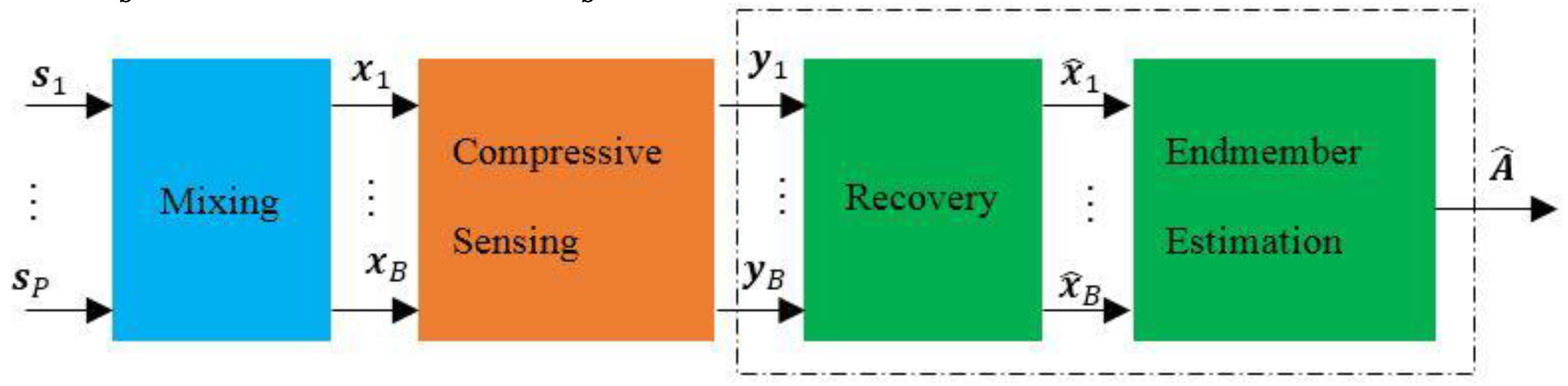
3.1. Framework Description of the Proposed Method

As discussed in Section 2, if we can estimate endmembers directly from the compressive HSI data without recovering the images, omitting the recovery step will greatly reduce the complexity of computation; we will obtain a much better estimation speed and possibly also a better estimation accuracy.
The compressive observation of HSI is denoted as follows:
Y = Φ X = Φ S A = [ Φ s 1 , Φ s 2 , , Φ s B ] A = [ v 1 , v 2 , , v B ] A = V A
where   v p =   Φ s p can be regarded as the compressive measurement of the source   s p .
The value y b = Φ x b = ( p = 1 P   v p a p b )   is the compressive measurement of mixture   x b , and it is also the mixture of all of the   v p ( p = 1 , 2 ,   , P ) . a p b is the element of matrix A at row p column b .
Equation (14) can be considered as LMM, as shown in Equation (3). Thus, we wish to estimate the endmember matrix   A directly via CG approaches such as PPI, N-FINDR, VCA, and MVCA.
Unfortunately, the properties of the measurement matrix Φ make it impossible to directly use the CG approaches on Equation (14). Incoherence is a critical property indicating that the structures of the measurement matrix used in CS that, unlike the signals of interest, have a dense representation in the basis   Ψ , and random matrices are largely incoherent with any fixed basis Ψ , making the sensing matrix   Θ   hold RIP with overwhelming probability [7]. Hence,   v p =   Φ s p is not sparse in basis   Ψ , and v [ n ] (similar to the definition of x [ n ] in 
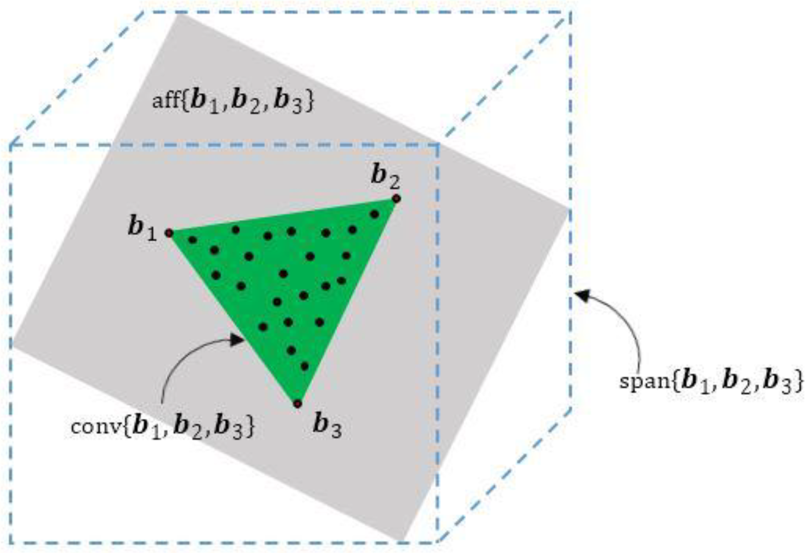
Section 2.1) cannot hold the non-negative and full additivity constraints, as shown in Equation (2), due to its dense and random character. We can see that:
y [ n ] C = { γ = i = 1 P v i [ n ] a i | v i [ n ] R } ,   n = 1 ,   2 , , N
v i [ n ] is the element in matrix V at column i row n . From Equation (15), we can see that C is not a convex hull, and y [ n ] is not a convex combination of endmember signatures. Actually, C is the space spanned by { a 1 , , a P } (see Figure 2 for the relationship between the spanned space and the convex hull), and y [ n ] is a point in the space. In this condition, the endmember signatures { a 1 , , a P } are no longer vertices of a simplex, which means that we cannot use CG approaches to estimate the endmembers directly.
To the knowledge of the authors and the referenced materials, we have not found a measurement matrix that not only satisfies the incoherence (or RIP), but also makes   v p =   Φ s p sparse in basis Ψ or   v [ n ] hold the non-negative and full additivity constraints. It seems impossible to estimate endmembers from compressive HSI data directly.
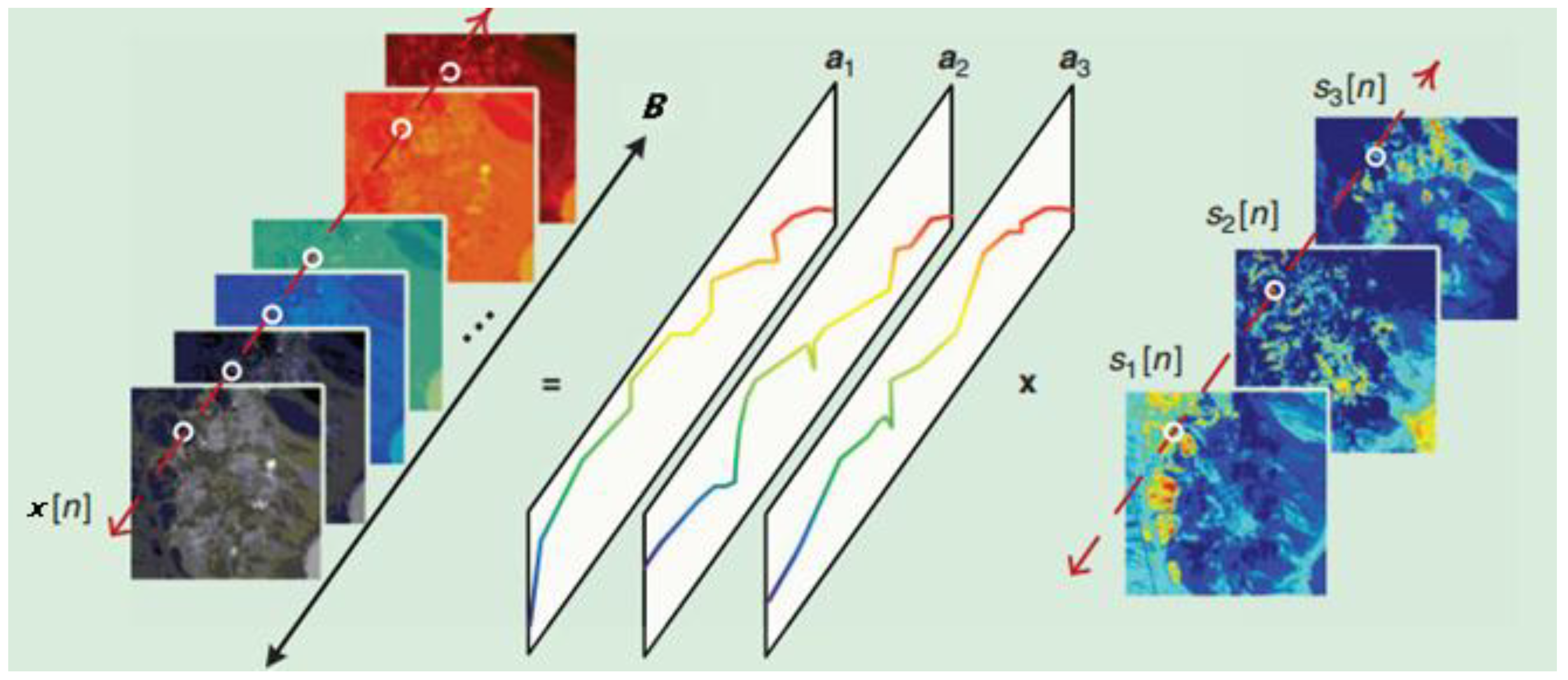
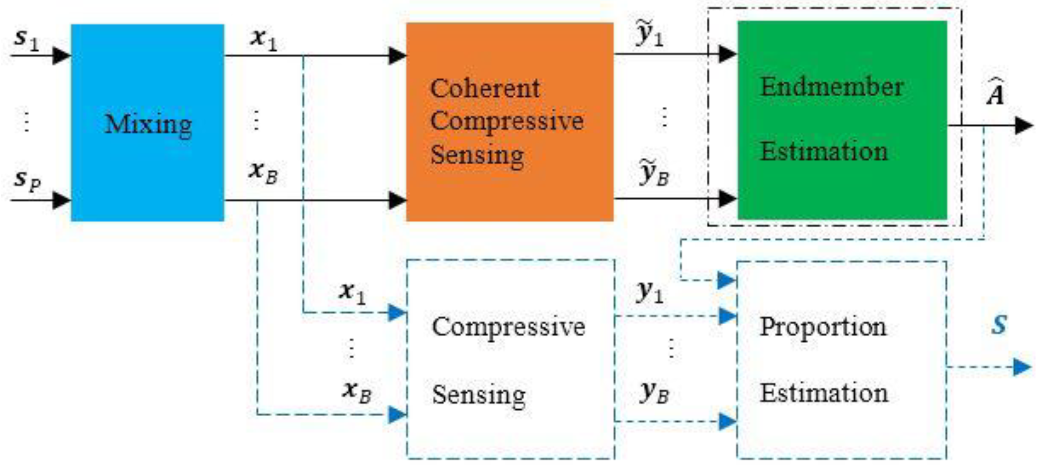
We propose a novel method, as shown in Figure 6. A coherent measurement matrix is used to compressively measure the HSI, and the endmembers can be directly estimated from the observations.
Figure 6. The framework of the proposed method.
Sensors 15 09305 g006
First, we design a coherent measurement matrix that makes   v [ n ]   hold the non-negative and full additivity constraints.
The coherent matrix that does not hold the RIP cannot be used for exact and robust signal recovery, as mentioned above. In this paper, the aim is to estimate endmembers directly from the compressive HSI data, not to recover the HSI data. Therefore, we do not have to use an incoherent matrix (meaning, we do not have to use a random matrix). We give an example of such a coherent matrix. Let I   ϵ   R N × N be an identity matrix. We construct the measurement matrix using parts of   I . For example, we select one row in every   t ( t = 1 ,   2 , ) rows from I to compose   Φ   ϵ  R M × N (the compression ratio is   t ,   M = round ( N t ) , where round() is the operation of rounding towards the nearest integer). It is clear that v [ n ] holds the non-negative and full additivity constraints. With this kind of measurement matrix, it is possible to use CG approaches, such as PPI or VCA, to estimate the endmembers directly by solving the problem shown in Equation (14).
Other measurement matrices Φ   that make v [ n ] in   V = Φ S hold the non-negative and full additivity constraints can be used in this proposed method.
This type of measurement matrix achieves undersampling of HSI. It will lose some proportion information. Therefore, the undersampled data cannot be used to recover the proportion information. If this information is required, one can recover it by the data captured by an incoherent measurement matrix, as shown in Figure 6.
In this paper, we use the VCA algorithm to estimate the endmembers directly in the proposed method. We assume the presence of pure pixels in the undersampled data as required by VCA, and we also assume the presence of all of the materials in the data. These assumptions are easy to realize for the increasing spatial resolution of hyperspectral sensors.
In the proposed method, we first use a coherent measurement matrix to compressively sense HSI and then use the VCA method to estimate the endmember directly from the HSI observations without recovering the images, which is a necessary step in the traditional method. As shown in the dashed parts in Figure 6, if the proportion information S is required, one can use another incoherent measurement matrix to capture the global information of HSI, which can be used along with the estimated endmembers A ^ to recover the proportions [5,20].

3.2. Analysis of the Computational and Memory Complexity

Under the linear observation model, HSI data are in a subspace of dimension   P . Typically,   P is far less than   B . The dimensionality B ranges from around 100 to 250, whereas P ranges from about 3 to 20 [29]. In the VCA algorithm, the HSI data dimensionality is reduced by PCA or SVD. The computational complexity of the proposed method is   O ( P 2 M ) [16].
The traditional methods used in this paper are SOMP-VCA (SOMP for HSI data recovery and VCA for endmember estimation) and OMP-MVCA. The computational complexity of the SOMP is   O ( B K M N ), where K is the sparsity of the signals. Typically, B and K are both larger than   P , so   B K M N > P 2 M N P 2 M . The computational complexity of VCA used in the traditional method is   O ( P 2 N ) (each spectral image length is N , while the length of the compressive spectral image in the proposed method is   M ). The total computational complexity of the traditional method is O ( B K M N + P 2 N ). In most cases,   B K M N > P 2 M N P 2 N , so the complexity can be simply denoted as   O ( B K M N ) . The computational complexity of the SOMP-VCA is much larger than that of the proposed method. P 2 N > P 2 M , and thus, we can see that the computational complexity of the traditional method is larger than that of the proposed method, even if we use other CS recovery methods besides the SOMP algorithm. The computational complexity of OMP is O ( B K M N ) when K N , otherwise, the computational complexity is the larger one of O ( B K 3 M ) and O ( B K M N ). The computational complexity of MVCA is smaller than that of VCA. So the complexity of OMP-MVCA is dominated by OMP.
In the proposed method, the memory required is O ( P M ) due to dimensionality reduction and data compression. In the SOMP-VCA method, the memory required by SOMP is O ( M N ) and the memory required by VCA is   O ( P N ) . M N P N > P M ; therefore, the memory required by the SOMP-VCA method can simply be   O ( M N ) , which is much larger than that of the proposed method. Similar to the analysis of SOMP-VCA, the memory required by OMP-MVCA is simply   O ( M N ) .

4. Simulation Results

4.1. Evaluations of the Proposed Method

In this section, we first evaluate the practicability of the proposed method. Then, we compare the performance of the proposed method with the performance of the SOMP-VCA method.
The data used in this paper are (1) the semi-synthetic HSI of a rural suburb of Geneva and (2) real-work urban HSI, both of which are also used in [5] (This dataset is available at [30]. We acknowledge Mohammad Golbabaee, Simon Arberet and Vandergheynst for providing the dataset.). In the rural HSI,   N = 64 × 64 ,   P = 3 ,   B = 64 , all the pixels are pure (which means that each pixel only contains one material), as shown in Figure 7. In the urban HSI,   N = 256 × 256 ,   P = 6 ,   B = 171 (the first 16 bands are used in this paper), and parts of the pixels are pure, as shown in Figure 8. In this paper, the size of HSI data is reduced by SVD from N × B to N × P in VCA algorithm.
Figure 7. The proportion of each material in the rural HSI.
Sensors 15 09305 g007
To evaluate the performance of the algorithms, we compute the rms (root-mean-square) error distance of vectors of angles   θ = [ θ 1 , θ 2 , , θ P ] T with
θ p = arccos a p , a ^ p || a p || · || a ^ p ||   , ( p = 1 ,   2 , , P )
where θ p is the angle between vector a p and a ^ p (the estimated value of a p ). Based on θ , we estimate the rms error distance:
rmsSAE  = ( 1 P p = 1 P ( θ p ) 2 ) 1 / 2
where rmsSAE measures the distance between a p and a ^ p for p = 1 ,   2 , , P . (SAE stands for the Signature Angle Error).
We use Φ ˜ to denote the coherent measurement matrix described in Section 3.1. In noisy cases, white Gaussian noise   n is added to the observation, i.e., Y ˜ = Φ ˜ X + n . The SNR (signal-to-noise ratio) is from 20 to 40 dB with a step length of 10 dB. N is the number of pixels of a hyperspectral image, and M is the number of compressive measurements of an image. The compression ratio t   ( t = round ( N M ) ) is from 2 to 20 with a step length of 1 in the proposed method. We also consider the non-compression (Nyquist sampling) data, i.e., t = 1 . Each experiment is repeated 50 times to calculate the mean result. The platform used in this paper is with the following hardware and software: (1) CPU: Intel Core i3 550, 3.2 GHz; (2) RAM: 4 GB; (3) OS: Windows 8, 64-bit; and (4) Matlab version: R2011b, 64-bit.
Figure 8. The proportion of each material in the urban HIS.
Sensors 15 09305 g008
From Figure 9 and Figure 10, we can see that as the compression ratio t grows, the rmsSAE does not change a lot, especially when the SNR is large, compared with the non-compression case t = 1 (this is due to the performance and the assumption of the VCA algorithm). However, the runtime decreases greatly as t increases compared with the non-compression case. We can see that the proposed method can estimate the endmember with comparable accuracy to the Nyquist-based method (t = 1) with much faster estimation speed as t increases, as long as the pure pixel and all material presence assumptions hold. We note that the value of t is user-defined as long as the presence of each material and pure pixel assumption holds.
To assess the performance of the proposed method for a large number of endmembers, we vary the number from P = 10 to P = 20 . The endmember data are mineral signatures extracted from the U.S. Geological Survey (USGS) spectral library [16]. Each endmember signature consists of B = 224 spectral bands. Each synthetic hyperspectral image has 4096 pixels.
From Figure 11 we can see that the rmsSAE values increase roughly with the increase of the number of endmembers under the same noise level. And the rmsSAE values also decrease roughly with the increase of SNR, as expected. Comparing Figure 11a,b, we can also see that the performance of the proposed is comparabe when t = 10 and t = 20 , as long as the pure pixel and all material presence assumptions hold.
Figure 9. (a) Rural HSI: the rmsSAE of the proposed method as a function of the compression ratio t with different SNR; (b) Urban HSI: the rmsSAE of the proposed method as a function of the compression ratio t with different SNR.
Sensors 15 09305 g009
Figure 10. (a) Rural HSI: runtime of the proposed method as a function of compression ratio t; (b) Urban HSI: runtime of the proposed method as a function of compression ratio t.
Sensors 15 09305 g010
Figure 11. The rmsSAE of the proposed method as a function of the number of endmembers under different noise levels. (a) Compression ratio t = 10; (b) Compression ratio t = 20.
Sensors 15 09305 g011

4.2. Comparison of the Proposed Method and the SOMP-VCA Method

Next, we compare the performance of the proposed method with the traditional SOMP-VCA and OMP-MVCA methods.
In SOMP-VCA and OMP-MVCA methods, the compression ratio t ranges from 2 to 10 with a step length of 2. The incoherent measurement matrix Φ T is a random Gaussian matrix [21]. Each of the six signals (endmembers) in the urban HSI data has   N = 65 , 536 points. They require too much memory, as described in Section 3.2, when processed by a computer (the computer used in the paper with 4 GB RAM cannot afford enough memory to run the SOMP-VCA/OMP-MVCA algorithm when t = 2 and 4). In the experiments below, we divide each signal into several segments, each of which consists of N T = 4906 points (The length of each signal in the rural HSI data is 4096). Therefore, Φ T is a M T × N T matrix, where   M T = round ( N T t ) . To recover the HSI data by the traditional method, the sparsity K of each segment is required as a priori condition. We set K = round ( N T 100 ) in the experiments (Generally, it is very hard for people to get the exact value of K in practical applications. This is also a disadvantage of traditional methods). In noisy cases, the SNR is from to 20 to 40 dB with a step length of 10 dB. Each experiment was repeated 50 times.
From Table 2 and Table 3, we can see that at the same compression ratio, the rmsSAEs of the proposed method are much smaller than the rmsSAEs of both SOMP-VCA and OMP-MVCA methods when it is used for both the synthetic and real data. The reason is that both SOMP-VCA and OMP-MVCA methods first recover the images and then estimate endmembers from the recovered images, and the recovery step will introduce error to the estimation step. The proposed method directly estimates the endmembers by the VCA method without the recovery step. We can see that in the noiseless case, the proposed method can estimate the endmembers exactly, as some values of rmsSAE in Table 2 and Table 3 are 0.0000.
Table 2. Rural HSI: the rmsSAE of the proposed method, SOMP-VCA method and OMP-MVCA method under different noise levels.
SNR (dB)MethodsCompression Ratio t
246810
20SOMP-VCA7.26558.564911.875616.514522.4027
OMP-MVCA9.457710.425413.682117.631723.6413
proposed method3.09572.95283.01542.96492.9956
30SOMP-VCA7.22718.761911.173616.124521.8981
OMP-MVCA9.037110.884212.909317.548022.7639
proposed method0.98580.94280.91470.87480.8937
40SOMP-VCA7.45248.581011.410715.757121.5858
OMP-MVCA9.160610.419112.972816.778622.8731
proposed method0.30220.30260.28530.28500.2823
noiselessSOMP-VCA7.13638.795511.150715.878821.1658
OMP-MVCA8.74269.706512.419116.297122.1178
proposed method0.00000.00000.00000.00000.0000
Table 3. Urban HSI: the rmsSAE of the proposed method, SOMP-VCA method and OMP-MVCA method under different noise levels.
SNR (dB)MethodsCompression Ratio t
246810
20SOMP-VCA24.918731.612936.083036.695237.4615
OMP-MVCA32.319434.422438.164441.180242.9744
proposed method13.576212.500611.972012.565012.2655
30SOMP-VCA26.157432.605235.946236.478838.6030
OMP-MVCA32.416834.677437.720641.175642.3880
proposed method8.42258.07818.24518.07528.1576
40SOMP-VCA25.234731.550335.562636.457437.4830
OMP-MVCA32.836235.357238.770641.415743.3261
proposed method5.02135.01314.65584.67364.7675
noiselessSOMP-VCA24.476032.273235.176337.274638.6559
OMP-MVCA31.752034.772638.842841.853943.3041
proposed method0.00000.06580.00000.06340.0000
Standard deviations of rmsSAE under different conditions are listed in Table 4 and Table 5. We can see that under the same condition, the standard deviation values of the proposed method are also smaller than the values of SOMP-VCA or OMP-MVCA methods. The results indicate that the convergence of the proposed method is the best among the three methods.
Table 4. Rural HSI: the standard deviations of rmsSAE of the proposed method, SOMP-VCA method and OMP-MVCA method under different noise levels.
SNR (dB)MethodsCompression Ratio t
246810
20SOMP-VCA0.89021.47991.76691.91002.4746
OMP-MVCA0.91731.40021.78101.94182.4016
proposed method0.29020.31090.28360.30090.2839
30SOMP-VCA1.12701.45651.87021.95822.1471
OMP-MVCA0.89751.47581.65971.86042.3451
proposed method0.09250.09460.08750.09370.1071
40SOMP-VCA0.95301.31301.70831.92892.4834
OMP-MVCA0.97191.90571.92872.47612.6789
proposed method0.02910.02950.03220.02730.0344
noiselessSOMP-VCA0.99901.46862.02722.26182.3057
OMP-MVCA0.96921.63012.02362.58432.4048
proposed method0.00000.00000.00000.00000.0000
Table 5. Urban HSI: the standard deviations of rmsSAE of the proposed method, SOMP-VCA method and OMP-MVCA method under different noise levels.
SNR (dB)MethodsCompression Ratio t
246810
20SOMP-VCA3.67385.70599.77199.684711.0516
OMP-MVCA5.84627.315610.507911.902912.2469
proposed method2.43301.85862.01412.20151.8326
30SOMP-VCA3.62215.72519.88479.816310.9784
OMP-MVCA5.87316.878910.541411.877912.2589
proposed method0.66610.78200.72650.59240.8368
40SOMP-VCA3.67855.86979.78969.816611.2482
OMP-MVCA5.74357.380010.619711.719812.6990
proposed method1.41821.23471.21491.25451.4128
noiselessSOMP-VCA3.55705.70079.81289.878611.2197
OMP-MVCA5.52447.569710.962311.813212.7545
proposed method0.00000.07810.00000.06730.0000
From Table 6 and Table 7, we can see that the time consumed by the proposed method is much smaller than the time consumed by SOMP-VCA or OMP-MVCA methods. As analyzed in Section 3, the proposed method estimates the endmembers in one step, while both SOMP-VCA and OMP-MVCA use two steps. Therefore, from Table 2 to Table 7, the estimation accuracy and speed of the proposed method are both better than those of SOMP-VCA and OMP-MVCA methods.
Table 6. Rural HSI: average runtime consumed by the two methods for estimating the endmembers.
Compression Ratio   t SOMP-VCAOMP-MVCAProposed Method
221.1327172.90770.0092
410.877996.58170.0076
67.446571.50780.0075
85.783958.45320.0075
104.795751.18180.0073
Table 7. Urban HSI: average runtime consumed by the two methods for estimating the endmembers.
Compression Ratio   t SOMP-VCAOMP-MVCAProposed Method
2113.5758692.25420.0287
459.8402385.94960.0168
641.8393285.09920.0143
832.9574233.93540.0130
1027.7860204.14610.0118
Different CS recovery algorithms affect the performance and the runtime for estimating the endmembers. To eliminate the influence of the choice of the CS method, we suppose that the sparsity of each signal is known and that the CS method can recover the HSI data accurately, and the recovered data are as accurate as the Nyquist-based data at the same noise level. From Figure 9 and Figure 10, we can see that the performance of the proposed method ( t > 1) is comparable to the performance of the method with Nyquist-based data ( t   = 1). Therefore, the performance of the proposed method is comparable to or better than the performance of the traditional CS base method. The same is true of the runtime time of the proposed method: it is less than that of the traditional CS base method with other CS recovery methods, as analyzed in Section 3.2.

5. Conclusions

In this paper, we proposed a new method to directly estimate the endmembers from the compressive observations of the HSI data, while traditional methods first have to recover the HSI data from the compressive observations and then estimate the endmembers. Simulation results demonstrated that the proposed method outperforms the traditional method with better estimation speed and better (or comparable) accuracy.

Acknowledgments

This work was supported in part by the National Natural Science Foundation of China under Grant 61102148.

Author Contributions

Hongwei Xu, Ning Fu and Xiyuan Peng conceived and designed the experiments; Hongwei Xu and Ning Fu performed the experiments and analysised the data; Hongwei Xu and Liyan Qiao wrote the paper.

Conflicts of Interest

The authors declare no conflict of interest.

References

  1. Eismann, M.T. Hyperspectral Remote Sensing; SPIE: Bellingham, WA, USA, 2012. [Google Scholar]
  2. Chang, C.I. Hyperspectral Data Exploitation: Theory and Applications; Wiley-Interscience: Hoboken, NJ, USA, 2007. [Google Scholar]
  3. Green, R.O.; Eastwood, M.L.; Sarture, C.M.; Chrien, T.G.; Aronsson, M.; Chippendale, B.J.; Faust, J.A.; Pavri, B.E.; Chovit, C.J.; Solis, M. Imaging spectroscopy and the airborne visible/infrared imaging spectrometer (AVIRIS). Remote Sens. Environ. 1998, 65, 227–248. [Google Scholar] [CrossRef]
  4. Tiangong-1 Service Platform for Promoting Space Utilization. Available online: http://www.msadc.cn (accessed on 10 October 2014).
  5. Golbabaee, M.; Arberet, S.; Vandergheynst, P. Compressive Source Separation: Theory and Methods for Hyperspectral Imaging. IEEE Trans. Image Process. 2013, 22, 5096–5110. [Google Scholar] [CrossRef] [PubMed]
  6. Donoho, D.L. Compressive sensing. IEEE Trans. Inf. Theory 2006, 52, 1289–1306. [Google Scholar] [CrossRef]
  7. Candes, E.J.; Wakin, M.B. An Introduction to Compressive Sampling. IEEE Signal Process. Mag. 2008, 25, 21–30. [Google Scholar] [CrossRef]
  8. Duarte, M.F.; Sarvotham, S.; Baron, D.; Wakin, M.B.; Baraniuk, R.G. Distributed Compressed Sensing of Jointly Sparse Signals. In Proceedings of the 39th Asilomar Conference on Signals, Systems and Computers, Pacific Grove, CA, USA, 30 October–2 November 2005; pp. 1537–1541.
  9. Baron, D.; Duarte, M.F.; Wakin, M.B.; Sarvotham, S.; Baraniuk, R.G. Distributed Compressive Sensing. Available online: http://arxiv.org/abs/0901.3403 (accessed on 21 April 2015).
  10. Baron, D.; Duarte, M.F.; Sarvotham, S.; Wakin, M.B.; Baraniuk, R.G. An information-theoretic approach to distribute compressed sensing. In Proceedings of the 43rd Allerton Conference on Communications, Control, Computer, Monticello, IL, USA, 28–30 September 2005; pp. 1–12.
  11. Keshava, N.; Mustard, J.F. Spectral unmixing. IEEE Signal Process. Mag. 2002, 19, 44–57. [Google Scholar] [CrossRef]
  12. Bioucas-Dias, J.; Plaza, A.; Dobigeon, N.; Parente, M.; Du, Q.; Gader, P.; Chanussot, J. Hyperspectral unmixing overview: Geometrical, statistical, and sparse regression-based approaches. IEEE J. Sel. Top. Appl. Earth Obs. Remote Sens. 2012, 5, 354–379. [Google Scholar] [CrossRef]
  13. Ma, W.K.; Bioucas-Dias, J.; Chan, T.H.; Gillis, N.; Gader, P.; Plaza, A.J.; Ambikapathi, A.; Chi, C.Y. A Signal Processing Perspective on Hyperspectral Unmixing: Insights from Remote Sensing. IEEE Signal Process. Mag. 2014, 31, 67–81. [Google Scholar] [CrossRef]
  14. Boardman, J. Automating spectral unmixing of AVIRIS data using convex geometry concepts. In Summaries 4th Annual JPL Airborne Geoscience Workshop; JPL Publication: Pasadena, CA, USA, 1993; Volume 1, pp. 11–14. [Google Scholar]
  15. Winter, M.E. N-findr: An algorithm for fast autonomous spectral end-member determination in hyperspectral data. In Proceedings of the SPIE Conference on Imaging Spectrometry V, Denver, CO, USA, 27 October 1999; pp. 266–275.
  16. Nascimento, J.M.P.; Dias, J.M.B. Vertex component analysis: A fast algorithm to unmix hyperspectral data. IEEE Trans. Geosci. Remote Sens. 2005, 43, 898–910. [Google Scholar] [CrossRef]
  17. Jia, S.; Qian, Y.T. Spectral and Spatial Complexity-Based Hyperspectral Unmixing. IEEE Trans. Geosci. Remote Sens. 2007, 45, 3867–3879. [Google Scholar] [CrossRef]
  18. Moudden, Y.; Bobin, J. Hyperspectral BSS Using GMCA with Spatio-Spectral Sparsity Constraints. IEEE Trans. Image Process. 2011, 20, 872–879. [Google Scholar] [CrossRef] [PubMed]
  19. Lopez, S.; Horstrand, P.; Callico, G.M.; Lopez, J.F.; Sarmiento, R. A low-computational-complexity algorithm for hyperspectral endmember extraction: Modified vertex component analysis. IEEE Geosci. Remote Sens. Lett. 2012, 9, 502–506. [Google Scholar] [CrossRef]
  20. Li, C.B.; Sun, T.; Kelly, K.F.; Zhang, Y. A Compressive Sensing and Unmixing Scheme for Hyperspectral Data Processing. IEEE Trans. Image Process. 2012, 21, 1200–1210. [Google Scholar] [CrossRef] [PubMed]
  21. Candès, E.J.; Romberg, J.; Tao, T. Stable signal recovery from incomplete and inaccurate measurements. Comm. Pure Appl. Math. 2006, 59, 1207–1223. [Google Scholar] [CrossRef]
  22. Shen, M.; Zhang, Q.; Li, D.; Yang, J.; Li, B. Adaptive sparse representation beamformer for high-frame-rate ultrasound imaging instrument. IEEE Trans. Instrum. Measur. 2012, 61, 1323–1333. [Google Scholar] [CrossRef]
  23. Candès, E.J.; Romberg, J.; Tao, T. Robust uncertainty principles: Exact signal reconstruction from highly incomplete frequency information. IEEE Trans. Inf. Theory 2006, 52, 489–509. [Google Scholar] [CrossRef]
  24. Kim, S.J.; Koh, K.; Lustig, M.; Boyd, S.; Gorinevsky, D. An interior-point method for large-scale l1-regularized least squares. IEEE J. Sel. Top. Signal Process. 2007, 1, 606–617. [Google Scholar] [CrossRef]
  25. Tropp, J.A.; Gilbert, A.C. Signal Recovery from Random Measurements via Orthogonal Matching Pursuit. IEEE Trans. Inf. Theory 2007, 53, 4655–4666. [Google Scholar] [CrossRef]
  26. Dai, W.; Milenkovic, O. Subspace pursuit for compressive sensing signal reconstruction. IEEE Trans. Inf. Theory 2009, 55, 2230–2249. [Google Scholar] [CrossRef]
  27. Aravind, N.V.; Abhinandan, K.; Achary, V.V.; Sumam, D.S. Comparison of OMP and SOMP in the reconstruction of compressively sensed Hyperspectral Images. In Proceedings of the 2011 International Conference on Communications and Signal Processing (ICCSP), Kerala, India, 10–12 February 2011; pp. 188–192.
  28. Tropp, J.A.; Gilbert, A.C.; Strauss, M.J. Simultaneous sparse approximation via greedy pursuit. In Proceedings of the ICASSP, Philadelphia, PA, USA, 19–23 March 2005.
  29. Zare, A.; Gader, P.; Gurumoorthy, K.S. Directly Measuring Material Proportions Using Hyperspectral Compressive Sensing. IEEE Geosci. Remote Sens. Lett. 2012, 9, 323–327. [Google Scholar] [CrossRef]
  30. Compressive Source Separation: Theory and Methods for Hyperspectral Imaging. Available online: http://infoscience.epfl.ch/record/180911 (accessed on 21 April 2015).

