Article

Genetic Diversity and Population Structure of a Wide Pisum spp. Core Collection

by
Nicolas Rispail
1,*,
Osman Zakaria Wohor
1,2,
Salvador Osuna-Caballero
1,
Eleonora Barilli
1 and
Diego Rubiales
1
1
Instituto de Agricultura Sostenible, CSIC, Avda. Menéndez Pidal s/n, 14004 Córdoba, Spain
2
Savanna Agriculture Research Institute, CSIR, Nyankpala, Tamale P.O. Box TL52, Ghana
*
Author to whom correspondence should be addressed.
Int. J. Mol. Sci. 2023, 24(3), 2470; https://doi.org/10.3390/ijms24032470
Submission received: 23 December 2022 / Revised: 19 January 2023 / Accepted: 25 January 2023 / Published: 27 January 2023

Abstract

:
Peas (Pisum sativum) are the fourth most cultivated pulses worldwide and a critical source of protein in animal feed and human food. Developing pea core collections improves our understanding of pea evolution and may ease the exploitation of their genetic diversity in breeding programs. We carefully selected a highly diverse pea core collection of 325 accessions and established their genetic diversity and population structure. DArTSeq genotyping provided 35,790 polymorphic DArTseq markers, of which 24,279 were SilicoDArT and 11,511 SNP markers. More than 90% of these markers mapped onto the pea reference genome, with an average of 2787 SilicoDArT and 1644 SNP markers per chromosome, and an average LD50 distance of 0.48 and 1.38 Mbp, respectively. The pea core collection clustered in three or six subpopulations depending on the pea subspecies. Many admixed accessions were also detected, confirming the frequent genetic exchange between populations. Our results support the classification of Pisum genus into two species, P. fulvum and P. sativum (including subsp. sativum, arvense, elatius, humile, jomardii and abyssinicum). In addition, the study showed that wild alleles were incorporated into the cultivated pea through the intermediate P. sativum subsp. jomardii and P. sativum subsp. arvense during pea domestication, which have important implications for breeding programs. The high genetic diversity found in the collection and the high marker coverage are also expected to improve trait discovery and the efficient implementation of advanced breeding approaches.

1. Introduction

Peas (Pisum sativum L.) are a multipurpose and low-cost source of protein, that have been an essential source of animal feed and human food for centuries [1]. It is the world’s fourth most cultivated pulse crop [2]. Their usage differentiates cultivated peas into dry peas, green peas and forage peas [3]. The most cultivated are dry peas, traditionally intended for animal feed, but increasingly becoming human food. North America dominates dry-pea production, followed by Europe, while the Asia-Pacific dominates green-pea production (https://www.fao.org/faostat/en/#home, accessed on 24 October 2022). Peas also improve the soil by fixing atmospheric nitrogen through symbiotic interactions with soilborne bacteria. These interactions have a beneficial impact on soil fertility and the nitrogen cycle [4]. Therefore, peas have an excellent potential to improve the livelihoods and protein requirements in regions with low–average protein supply per capita and day. However, pea yield is still unstable due to its limited adaptability to various environmental conditions and susceptibility to diseases and pests. Therefore, great efforts are needed to improve its adaptation and resistance to biotic and abiotic stresses [1,5].
Peas are among the world’s oldest domesticated crops, with evidence of domestication dating back 10,000 years. The crop centre of origin and diversity is the Near East, with secondary diversification regions in the Mediterranean and East Africa. Pisum is a member of the family Fabaceae, the subfamily Papillionaceae, and the tribe Vicieae. The taxonomy of the genus Pisum is very complex and still under debate, with some authors recommending its inclusion in the genus Lathyrus [6]. It is generally accepted that Pisum includes three species: P. sativum, P. fulvum and P. abyssinicum [7,8,9]. However, the status of P. abyssinicum as an independent species, or as a P. sativum subspecies, is still controversial [10]. P. sativum is the primary and more diverse species of the genus. This species has been recently separated into two subspecies: subsp. sativum that contains cultivated peas and subsp. elatius that contains wild peas [11]. Each P. sativum subspecies is further divided into varieties, including the cultivated var. sativum and var. arvense, and the wild var. elatius and var. pumilio [7], a synonym of P. sativum var. humile and P. sativum var. syriacum [12,13]. Additional wild subspecies have also been described, including subsp. jomardii [14], subsp. thebaicum, subsp. transcaucasicum, subsp. asiaticum and subsp. cinereum, although their taxonomy status remains unclear.
All Pisum species and subspecies are crossable, albeit fertile hybrids between wild and cultivated peas may be obtained at a low rate [15]. Breeding programs may benefit from this wealth of natural diversity. Many ex situ pea germplasm collections have been developed to provide long-term conservation and ready access to a broad range of diversity [8]. These collections include wild, local landraces, commercial varieties and mutants. They are rich in genetic diversity for many traits of agronomical interest, including growth habits, seed quality and resistance to stress [16]. Several core collections have been developed to facilitate pea breeding programs [3,8,17], that significantly improve pea yield and quality through classical breeding [3,16].
Several approaches have been applied in pea breeding programs, including bulk selection, pedigree breeding schemes through transgressive segregation, single-seed descent and backcross selection, for scouting single dominant traits [2]. More recently, molecular marker technology has introduced new dimensions for improving traits of interest [2]. This technology facilitates genetic diversity studies to provide essential information for genetic conservation and efficient breeding of new commercial varieties [2,18]. They also allow for the deployment of linkage maps that localize specific genetic regions in the genome, and identify flanking markers associated with valuable traits [18]. Extensive genetic maps have been established based on bi-parental mapping populations combining different markers, including morphological markers, isozymes, RFLPs, RAPDs, SSRs and SNPs [19]. The knowledge collected from these markers led to the development of a consensus composite map of 1430 cM, comprising 239 microsatellite markers helpful in locating QTLs controlling disease resistance, as well as quality and morphological traits [19].
More recently, advances in sequencing technology opened the possibility of implementing genome-wide association studies (GWAS) and genomic selection (GS) to facilitate and boost future QTL identification and breeding [2]. The efficient implementation of these advanced breeding approaches depends on the molecular markers’ genome coverage, the extent of linkage disequilibrium (LD) between these markers and the population structure of the germplasm collection [20,21]. In addition, germplasm collections should contain high genetic diversity with a wide variation for the traits of interest. A detailed description of genetic diversity and population structure is a crucial prerequisite to their implementation [20]. Furthermore, genetic diversity is a significant determinant of a species’ capacity to persist and adapt to their environment. Unravelling genetic differentiation factors may explain how species react to changing environments [22]. Many studies aimed to clarify the genetic diversity of peas with diverse molecular markers and germplasm core collections [2]. The results of these studies were highly variable depending on the composition of the collection and the method employed. However, they all demonstrated a high genetic richness within peas and highlighted the complex population structure that explains the unresolved pea taxonomy [23,24].
In this work, we established the population structure and genetic diversity of a pea core collection containing 325 accessions from a worldwide origin. The collection includes all Pisum species and subspecies, to shed further light on the pea phylogenetic relationship, and serve as a first step toward implementing GWAS and GS in peas for agronomic traits and disease resistance.

2. Results

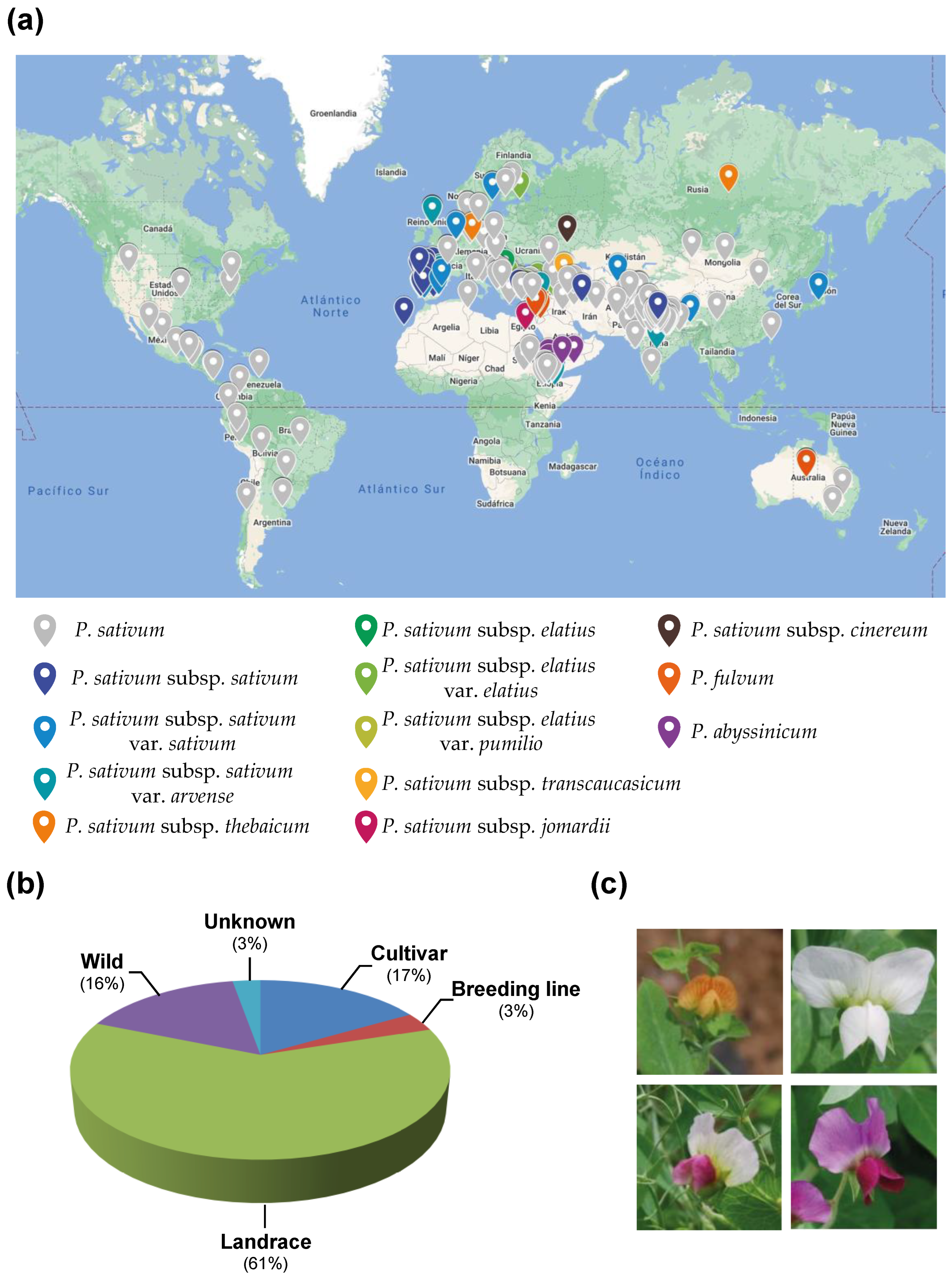
2.1. The Pea Core Collection

The Instituto de Agricultura Sostenible (IAS) pea core collection contained 325 accessions. Pea accessions of this core collection were selected based on geographical and morphological diversity to preserve the underlying levels of genetic diversity. Disease resistance was at the base of the germplasm-gathering process. Therefore, previously described sources of disease resistance including powdery mildew, rust, ascochyta blight, fusarium wilt and broomrape, were included in the core collection [25,26,27,28,29]. Although some commercial varieties and breeding lines were included, the predominant accessions were landraces, representing 61% of the collection. Wild species represented 16% of the collection. The collection was further selected based on flower-colour variability and contained accessions with white, purple, pink, lilac and orange flowers (Figure 1, Table 1 and Supplementary Table S1). Preliminary evaluation of this collection to rust showed a wide variety of responses, from susceptible to resistant accessions, indicating its suitability for further genetic study of disease resistance [30].

2.2. DArTSeq Marker Sequencing and Genetic Diversity Indices

DArTSeq sequencing and assembling of the collection led to the identification of 66,643 SilicoDArT and 55,269 SNP markers. After the stringent data curation according to minor allele frequency (MAF), heterozygosity and missing values, 24,279 polymorphic SilicoDArT markers and 11,511 SNP markers were obtained. Mapping these DArTSeq markers onto the pea reference genome located 19,514 SilicoDArT and 10,125 SNP markers on the seven pea chromosomes (82.8% of the DArTSeq markers). In addition, 2703 SilicoDArT and 1155 SNP mapped to unanchored pea contigs and supercontigs (10.8% of the DArTSeq markers), while 2062 SilicoDArT and 231 SNP markers remained unaligned (6.4% of the DArTseq markers). Sequence read data from these accessions are available at the NCBI SRA archive as BioProject PRJNA890072. The DArTSeq marker datasets were deposited in the public Zenodo depository [31].
To estimate the genetic diversity of the IAS pea core collection, we estimated the polymorphic information content (PIC), MAF, allele richness (Ar), expected heterozygosity (He), observed heterozygosity (Ho) and inbreeding coefficient (FIS) for each DArTSeq marker (Table 2). Wide variability for all parameters evaluated was observed across markers. For SilicoDArT, PIC values varied from 0.006 to 0.499, with an average value of 0.295, while MAF varied from 0.052 to 0.997, with a mean value of 0.41. He values were slightly lower than PIC, varying from 0 to 0.5, with a mean value of 0.217. Wide variation was also observed for the inbreeding coefficient that varied from −0.102 to 1, with a mean value of 0.692. Results obtained for SNP markers were broadly similar to those estimated for SilicoDArT markers (Table 2).

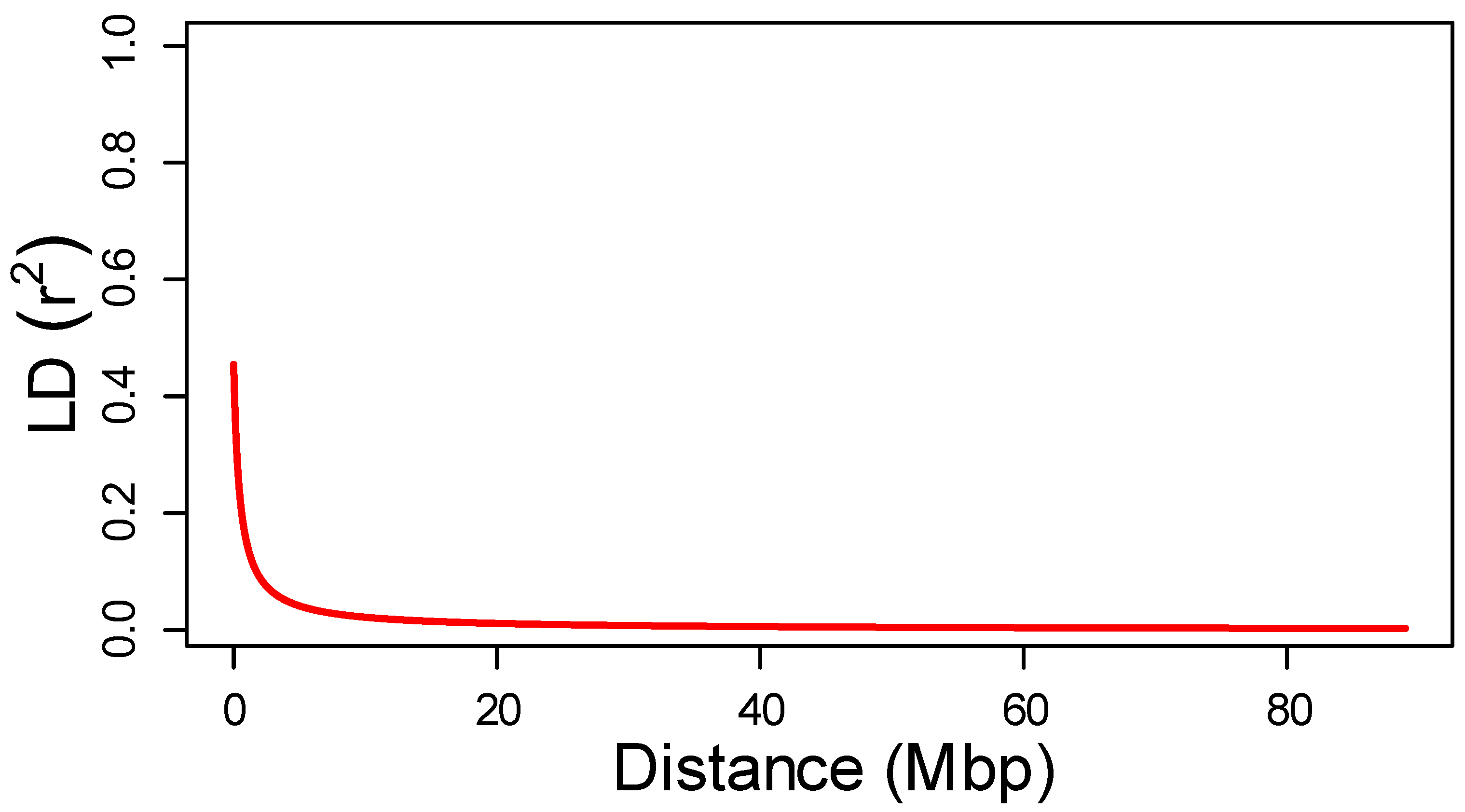
2.3. Marker Distribution and Linkage Disequilibrium

DArTSeq marker distribution over the pea genome showed a homogeneous distribution, covering the full length of the seven chromosomes (Supplementary Figure S1 and Table 3). Although the coverage of both marker types was similar, the density of SilicoDArT markers doubled that of SNP markers (Table 3). The average number and distance between SilicoDarT markers were circa two-fold that of SNP markers, reaching 2787.7 markers per chromosome, separated by 0.166 Mbp for SilicoDArT markers and 1446.4 markers, separated by 0.319 Mbp for SNP markers, respectively (Table 3). Slight variations were also detected in the marker distribution between chromosomes, with chromosome 2 presenting the lowest values and chromosome 5 the highest (Table 3). Interestingly, the middle region of chromosome 2 was inferior in molecular markers.
Inspection of intra-chromosomal linkage disequilibrium (LD) indicated that r2 varied from 0.012 to 1 for both SilicoDArT and SNP markers. The mean LD value and the overall critical value of LD (r290), estimated as the ninetieth percentiles of r2, were also similar between marker types reaching values of 0.103 and 0.236 for SilicoDArT, and 0.118 and 0.28 for SNP markers, respectively (Table 4). Plotting the r2 value over the physical distance between markers shows the rapid LD decay reaching LD50, at 0.48 and 1.38 Mbp for SilicoDArT and SNP markers, respectively (Figure 2). Estimation of LD by chromosomes shows slight differences in the extent of marker linkage between chromosomes. Chromosome 6 showed the highest LD50, mean r2 and r290 values, while chromosome 7 showed the lowest (Table 4, Supplementary Figure S2).

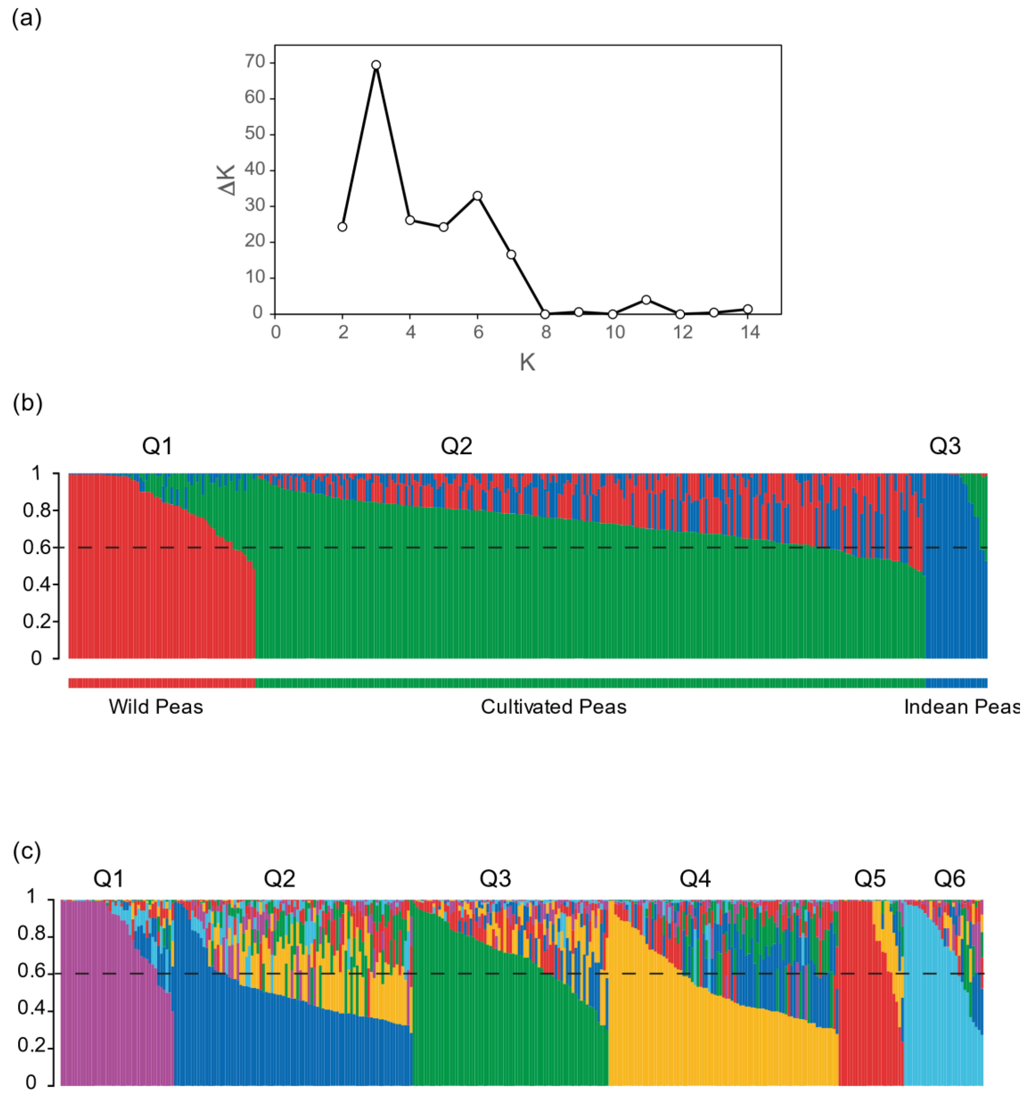
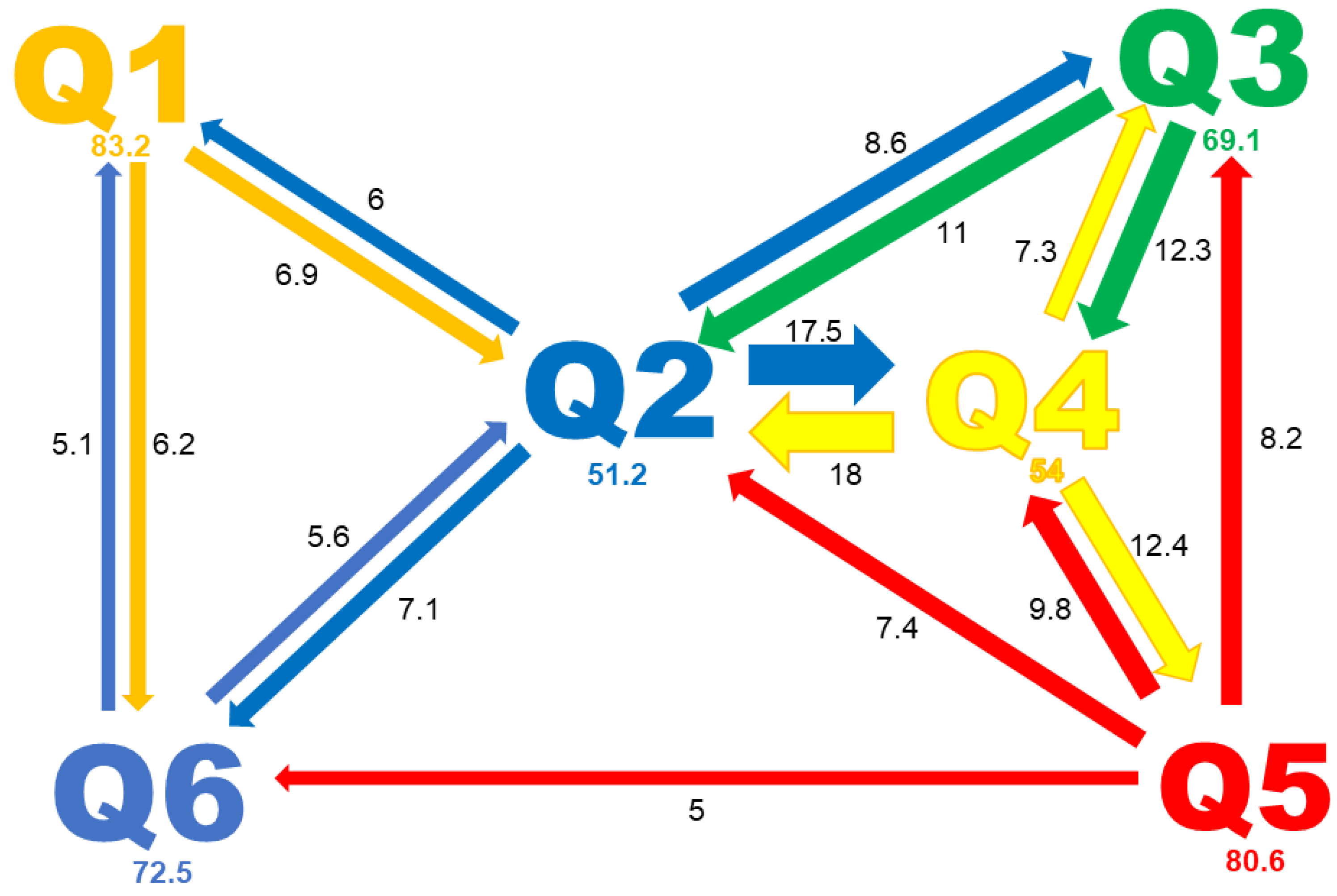
2.4. Genetic Structure of the Pea Core Collection

The genetic structure of the pea core collection was analysed with the model-based software STRUCTURE after LD pruning of the SilicoDarT marker matrix, as this database showed the highest chromosomal coverage. The evolution of the Evanno parameter (Δk) showed two peaks, suggesting the presence of three or six subpopulations (Figure 3a). According to STRUCTURE output for K = 3 (Figure 3b and Table 5), the first group (Q1), containing 28.16% of the collection, was constituted by wild pea relatives, including all accession of P. fulvum, P. abyssinicum, P. sativum subsp. elatius var. pumilio, P. sativum subsp. transcaucasicum and most P. sativum subsp. elatius var. elatius accessions. The second group (Q2), representing 56.83% of the collection, contained the cultivars and landraces of P. sativum subsp. sativum var. sativum, P. sativum subsp. sativum var. arvense, P. sativum subsp. jomardii, P. sativum subsp. thebaicum and P. sativum subsp. cinereum. This group included six P. sativum subsp. elatius var. elatius accessions; two had a shared membership percentage (circa 50% Q2 and 45% Q1). The third group (Q3), containing 15.01% of the collection, was composed of a smaller set of P. sativum landraces from India (Figure 3b and Table 5).
For K = 6, the group of wild accessions was further divided into two, representing 14.25 and 9.37% of the collection, respectively (Figure 3c and Table 4). The first sub-group (Q1) contained the P. fulvum and P. abyssinicum accessions and most of the P. sativum subsp. elatius var. elatius. By contrast, the second and smallest wild sub-group (Q6) contained the P. sativum subsp. elatius var. pumilio accessions [11]. At K = 6, the group of the cultivated subspecies was also separated into three sub-groups, each representing 21% of the collection (Table 5). The first one (Q2) contained landraces of P. sativum, all accessions from the P. sativum subsp. jomardii and thebaicum, and two accessions initially assigned to P. sativum subsp. elatius. The second sub-group (Q3) contained the P. sativum subsp. sativum var. sativum cultivars, while the last sub-group (Q4) contained all the landraces from P. sativum subsp. sativum var. arvense. Finally, the Indian P. sativum landraces, that represented 12% of the collection, composed the Q5 sub-group (Figure 3c).
This analysis also revealed a high level of admixture, with 46 and 155 accessions showing a percentage of membership to any subpopulation lower than 60% for K = 3 and 6, respectively. Most accessions with less than 60% of membership to a given group were assigned to Q2 and Q4, which represented 78.6% and 68% of admixed accessions, respectively. The proportion of admixed accessions for the other groups was lower than 30%. The mean membership percentage was 51.2% and 54% for Q2 and Q4 (Figure 4), approximately 70% for Q3 and Q6, and above 80% for Q1 and Q5. This analysis also revealed that members of the Q2 subpopulation shared genetic information with all other subpopulations. This subpopulation of domesticated peas shares approximately 6% of genetic information with each of the wild subpopulations (Q1 and Q6). None of the other domesticated pea subpopulations showed evidence of sharing significant genetic information with these wild subpopulations. By contrast, Q2 and Q4 shared approximately 18% of genetic information from each other. This analysis also revealed an important shared history between Q4, Q3 and Q5 subpopulations (Figure 4).
Estimation of the fixation index (Fst) for each subpopulation pointed to the significant divergence between subpopulations (Table 5). Estimated Fst values ranged from 0.2268 to 0.4315 for K = 3, and from 0.3316 to 0.5404 for K = 6, respectively (Table 5). The genetic distance between accessions within each subpopulation varied from 0.1514 to 0.2262 for K = 3, and from 0.1305 to 0.2141 for K = 6 (Table 5).

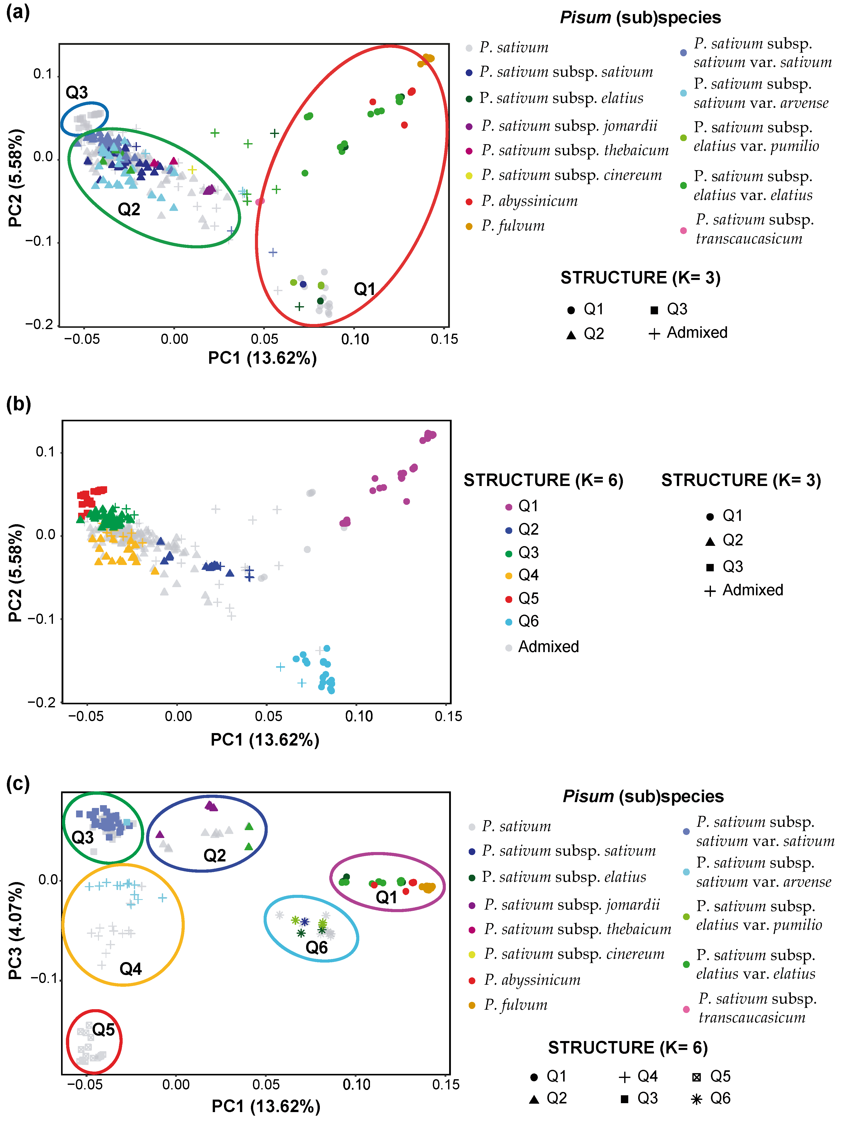
2.5. Principal Component Analysis

To clarify the genetic structure of the pea core collection, principal component analysis (PCA) was performed to highlight the different variables that could explain the splitting of this population. The initial three principal components (PCs) explained 23.3% of the observed genetic variation in the pea collection. The first PC explained up to 13.62% of the variation, the second explained 5.58 and third PCs explained 4.07%. The first two PCs clustered the pea collection in three different groups (Figure 5a,b). The first group included P. fulvum, P. sativum subsp. elatius var. elatius and P. abyssinicum accessions. The second group contained the P. sativum subsp. elatius var. pumilio. The last, and most significant group, contained domesticated P. sativum.
Superposing the STRUCTURE clustering for K = 3 or K = 6 to the PCA clustering favours the estimation of six subpopulations (Figure 5b). In this case, the two smaller PCA groups corresponded to the STRUCTURE subpopulation Q1 and Q6 respectively. The other STRUCTURE subpopulations were included within the leading PCA group in four distinct clusters (Figure 5b). The presence of six subpopulations was further supported after plotting PC1 vs PC3 which revealed six clusters, corresponding to the six subpopulations previously estimated by STRUCTURE for K = 6 (Figure 5c).

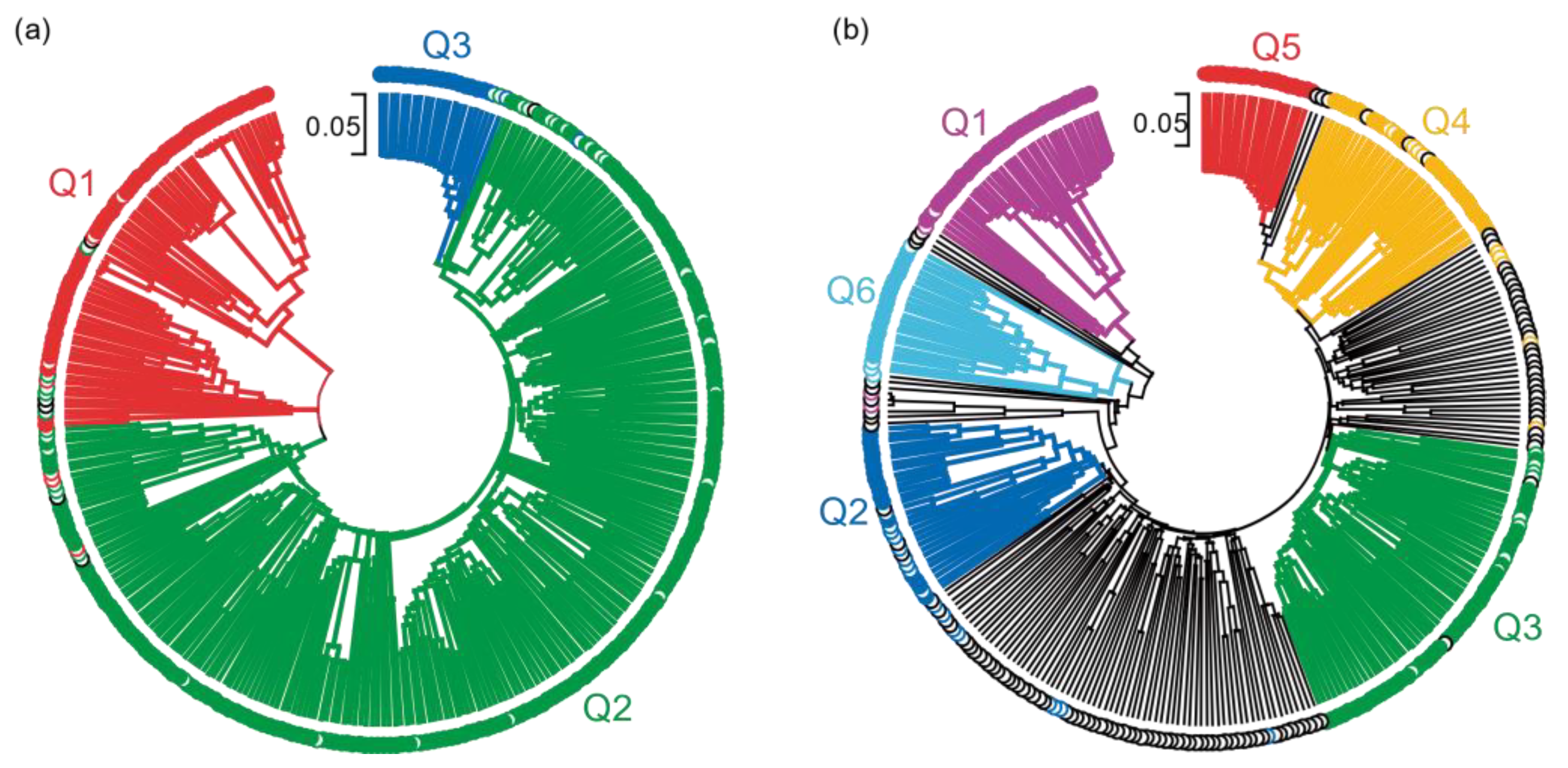
2.6. Phylogenetic Relationship of the Pisum Core Collection

The Neigbor-Joining (NJ) tree resolved into six distinct groups, as shown in Figure 6. Comparing the NJ tree with the STRUCTURE and PCA results revealed considerable congruence. For K = 3, subpopulation 1 was formed by two distinct clusters located at the base of the phylogenetic tree. Subpopulation 2 was composed of four distinct clusters. Subpopulation 3 appeared as a small cluster closely related to subpopulation 2, further supporting the PCA results (Figure 6a). The congruence between PCA, STRUCTURE and the phylogenetic analysis was more robust for K = 6 where each STRUCTURE subpopulation corresponded to distinct clusters on the NJ phylogenetic tree (Figure 6b). Interestingly, each subpopulation was separated by admixed accessions (% membership < 60%), supporting a significant history of hybridization and mixture between populations along evolution. Similarly, subpopulation 2 clustered between wild and domesticated pea subpopulations, while Q4 was located between Q3 and Q5.

3. Discussion

Broadening crop genetic diversity is critical for efficient breeding. Therefore, the conservation and characterisation of crop genetic resources is a crucial breeding element. The development of core collections representative of the crop genetic diversity allows the successful exploitation of genetic diversity richness, and protects against genetic erosion. These core collections, therefore, represent unique genetic diversity donors to enhance genetic gain, boost production and reduce stress-induced losses [17,32,33]. The constant cost decrease and higher efficiency of crop genotyping significantly increase the opportunity to characterise and exploit these collections. Although phenotypic evaluation is still a prerequisite to their efficient exploitation, incorporating genetic maps with high-density marker coverage and efficient bioinformatic tools can optimize their evaluation and usefulness [32,33].
Despite pea agronomic importance and long cultivation history, its domestication events and population dynamics still need to be better understood [22,24]. The development of diverse pea core collections and their detailed characterisation at genetic and population-genomic levels are improving our understanding of pea evolutions, and may ease their wide exploitation in breeding programs through the implementation of quantitative genomic approaches (GWAS and GS) [8,17,32]. The large size and complexity of the pea genome have largely delayed genomic research on this crop compared to other crops. However, the recent development of NGS-based genotyping facilitates the development of thousands of genome-wide molecular markers. In addition, the release of the pea reference genome sequences increased the scientific community’s interest, rapidly closing the gap, providing new insights into pea domestication and boosting pea breeding [2,9,17,34]. Accordingly, the carefully selected pea-core collection was extensively analysed for genetic diversity and population structure (Figure 1). This collection was designed to widen the available pea genetic diversity and exploit disease resistance traits. Therefore, the previously-described source of (partial) resistance to the most prevalent pea diseases was included in the collection. This collection partially overlaps with previously-developed pea panels designed to untangle pea domestication history [24,35] or contribute to pea breeding [17,20]. Eighty accessions (24.6% of the collection) are shared in at least one previously-described pea panel, which allows comparing and integrating the results of the different studies to get further insight into the pea genetic diversity and population dynamics.
DarTSeq genotyping approach has emerged as a proper genomic method for GS, genetic mapping and population genetics approaches in many plant species [36,37]. Application of this GBS-related approach in the present study provided a high-density coverage of the pea genome and yielded reliable data. It allowed for the generation of 35,790 polymorphic DArT markers, of which 24,279 were SilicoDArT and 11,511 SNP markers. These results were similar to previous studies on a pea panel genotyped with the DArTSeq approach that identified 35,647 DarT markers [24] and 11,343 SNP markers [35]. It was also similar to the number of SNP markers obtained from pea panels with the widely used Genopea Infinium SNP array [23,38,39], and in the same order of magnitude as the GBS approach [32,40]. In addition, estimation of the genetic diversity DArTSeq markers harbour moderate level of genetic diversity, with PIC and He mean values of 0.295 and 0.217, respectively. However, the genetic diversity harboured by each marker varied largely (Table 2), which is similar to previous studies using DArTSeq technology [41,42]. As such, our results confirm the capacity of DArTSeq to provide high-throughput genome-wide polymorphism markers.
Interestingly, the total number of DArTSeq markers collected here was three-fold higher than a previous DArT sequencing of peas based on several RIL populations [37]. The ratio between SilicoDArT marker and SNP markers was broadly similar between both studies. This difference in the total number of polymorphic markers between diverse pea collections and RILs was in accordance with previous results, confirming the lower RIL population genetic variability [40,43].
More than 90% of the DArT markers could be mapped onto the seven pea chromosomes and unaligned supercontigs. The alignment of DArTSeq markers onto the reference pea genome showed good coverage of all pea chromosomes. We observed an average of 2787 SilicoDArT and 1644 SNP markers per chromosome, evenly distributed across the chromosomes, which is in accordance with previous studies on peas (Table 3) [38]. A high number and genome-wide distribution of molecular markers are paramount for subsequent quantitative genomic approaches, such as GWAS and GS. The high number of markers and their broadly-even distribution onto the pea chromosomes, with the polymorphic markers detected here, should allow the successful implementation of GWAS and GS approach with this pea core collection.
Population structure and LD are the main obstacles to identifying significantly-associated markers with phenotypic traits [44]. The power of association studies depends on the existing LD between the gene(s) controlling phenotypic trait(s) and associated marker(s). Our data showed an extensive LD between markers. The LD-decay estimates on the seven pea chromosomes varied from 0.24 to 1.05 Mbp (mean 0.48 Mbp; Figure 2 and Table 4), which represented approximatively from 0.04 to 0.19 cM (mean 0.09 cM), agreeing with previously-estimated correspondence of 1 cM per 5.6 kb [23]. A recent study obtained after the pea reference genome release indicated a significantly smaller distance of LD decay, varying from 0.03 to 0.18 Mbp [40]. However, this difference in the LD-decay distance may be due to differences in the method used to estimate the LD50 distance. In the present study, LD50 distance corresponded to the physical distance in Mb at which LD had decayed to half of the r2 max. At the same time, it was limited to the r2max,90 in the previous study, because the r2max,90 for each chromosome was similar between both studies (Table 4) [40]. Additionally, our LD50 estimation was in the same order of magnitude as previous studies that estimated an LD50 distance between 0.05 to 0.9 cM, depending on the pea panel [23,38,39]. The rapid LD decay and the high chromosomal coverage, with markers at an average of 0.166 Mbp within the LD-decay window, should ensure the efficient and precise delineation of QTLs in future GWAS studies.
Population structure analysis of the IAS pea core panel through PCA, STRUCTURE and phylogenetic approaches differentiated three or six subpopulations (Figure 3, Figure 5 and Figure 6). This study also uncovered many admixtures with nearly half of the pea accessions having less than 60% membership to any subpopulation for K = 6. These results confirm the reproductive compatibility existing between Pisum species and subspecies [11]. They also indicated that even if self-pollination is the predominant mode of reproduction and some reproductive barriers exist, hybridization between accessions from different Pisum species and subspecies frequently occurred during pea evolution and domestication [11,24,35,45]. The Evanno’s method used to determine the number of pea populations from STRUCTURE revealed a major peak of Δk for K = 3 and a secondary peak at K = 6 (Figure 3). This indicated that the pea core panel was composed of three main populations (Figure 3). The wild pea accessions, at K = 6, included the species P. fulvum and P. abyssinicum, and the wild P. sativum subsp. elatius clustered together in one group (Q1). Cultivated P. sativum, including P. sativum subsp. sativum var. sativum and P. sativum subsp. sativum var. arvense clustered in two additional groups (Q2 and Q3). The Q2 clustered most of the cultivated P. sativum accessions, and the Q3 were pea landraces from the northern regions of India. This clustering was supported by the phylogenetic analysis, while the PCA results separated the wild population into two distinct groups, suggesting additional genetics clusters (Figure 5). The lower number of populations estimated by STRUCTURE may be due to the approximation used by the Evanno’s method that often underestimates the number of genetic clusters [46,47,48,49].
Accordingly, the three main groups of the pea core panel can be further differentiated into six clusters separated by the NJ trees and the PC1 vs. PC3 representation of the PCA analysis. In this latest analysis, PC1 discriminated accessions based on their domestication degree (wild or domesticated), while PC3 discriminated among the subspecies. In this grouping, the wild group was separated into two clusters. The first cluster contained the P. fulvum, P. abyssinicum and most accessions of P. sativum subsp. elatius var. elatius (Q1). The second included all accessions assigned to P. sativum subsp. elatius var. pumilio (Q6). The division of these two varieties confirmed their genetic distinctiveness, as previously shown by examining several wild populations from Israel and other Mediterranean regions that differentiated between P. sativum subsp. elatius var. elatius and P. sativum subsp. elatius var. humile [22,50].
On the other hand, the domesticated groups formed four distinct clusters. This result confirmed the genetic distinctiveness of the subset of Indian P. sativum accessions that formed the Q5 cluster. Central Asia (covering the highland Asiatic region from Afghanistan, the Hindu Kush and along the length of the southern slopes of the Himalayan mountains, as well as the central areas of China) is a relevant secondary centre of pea diversity that is thought to be rich in primitive cultivated forms of field peas [51,52]. Previous population genomics studies on these regions demonstrated a greater diversity within these regions than worldwide [51], providing evidence for the existence of separate gene pools from northcentral China and Afghanistan [13,52]. A similar situation might exist in Indian northern regions, given the geographical proximity, leading to this separated pea gene pool. The overlapping of the pea panels used for these different studies hamper the comparison of the genetic diversity held between these different central-Asian gene pools. Therefore, further studies targeting central Asia would be needed to clarify the relation between these gene pools and reconstruct their domestication history.
The rest of the domesticated accessions were divided into three clusters; one containing all the P. sativum subsp. sativum var. sativum cultivars and landraces (Q3), and two large groups of highly admixed accessions containing the P. sativum subsp. jomardii (Q2) and P. sativum subsp. sativum var. arvense (Q4). Most accessions assigned to Q2 and Q4 by STRUCTURE showed a membership coefficient lower than 60%; 78.6% of the Q2 accessions and 68% of the Q4 accessions were admixed. The percentage of admixed accessions from other clusters only varied from 15 to 30%. Further examination of the individual membership coefficient from each cluster indicated many hybridization events between Q2 accessions and the wild subpopulations (Q1 and Q6). The results revealed the existence of a frequent genetic exchange between Q2 and Q4, and between Q4 and the other two domesticated clusters (Q3 and Q5) (Figure 4). This suggests that P. sativum subsp. jomardii and P. sativum subsp. sativum var. arvense subpopulations arose during pea domestication, and are intermediate populations between the wild and domesticated genotypes. Therefore, these two subpopulations have a high potential for pea breeding. Our results for the Q2 subpopulation support and illustrate the condition of P. sativum subsp. jomardii as a domestication intermediate, previously proposed by Kosterin and co-workers [14,53].
All previous population genetic analyses separated the wild from domesticated peas and, depending on the scope of the study, further separated the wild or the domesticated pea accessions into several clusters. Depending on the study, pea accessions were grouped based on their species/subspecies [13,22,35], geographic origin [50] and end-use or sowing types [20,38]. The present study separated wild and domesticated pea accessions and separated each group into two and four subpopulations (Figure 3 and Figure 5). While two wild subpopulations were detected, our data could not separate the P. fulvum and P. abysinicum from the wild P. sativum subsp. elatius var. elatius accessions in contrast with most previous studies [22,35], although all P. fulvum clustered together in a slightly separated group within Q1 (Figure 3). This might be due to the relatively-low number of accessions belonging to P. fulvum and P. abysinicum contained in the IAS pea core collection. For the other subpopulations, pea accessions were separated based on the P. sativum subspecies, with P. sativum subsp. sativum var. arvense forming Q4 and the P. sativum subsp. jomardii and P. sativum subsp. thebaicum forming Q2. Although the overlapping between the IAS pea core collection and the USDA collection was limited, the percentage of accessions from each Pisum subspecies was similar between both core collections. Accordingly, the PCA analysis produced identical results (Figure 5a), apart from the P. fulvum accessions [17]. Similarly, no clustering based on the geographic origin of the accessions could be detected from our data, except for Q5 (Figure 3) [17]. The IAS core collection mostly contained landraces and wild accessions, with limited passport information related to end-uses and sowing types. The available information showed no clear grouping from end-uses or sowing types, although all winter peas clustered in Q2 (Supplementary Table S1).
The present study supports several taxonomic considerations. Firstly, many studies demonstrated that the domesticated P. abyssinicum is distinct from P. sativum and arose from an independent domestication event [35,54]. However, the two species shared several agronomy traits, such as pod indehiscence and the lack of seed dormancy [10]. Consequently, Weeden [10] postulated that “if forms of wild ‘elatius’, which is largely divergent from P. sativum subsp. sativum, is not defined at the species level, there is no justification for defining P. abyssinicum as a species either”. Therefore Weeden [10] proposed its classification as a subspecies within P. sativum. In our study, the P. abyssinicum accessions could not be differentiated from the P. sativum subsp. elatius accessions (Figure 3 and Figure 5). This result suggests that the genetic differences between the “abyssinicum” and “sativum” forms and the “elatius” and “sativum” forms are similar, and agrees with Weeden’s considerations. Several studies targeting the origin of the Abyssinian peas also supports Weeden’s taxonomic classification [35,54], although others favoured its consideration as a species [7,9]. Secondly, the taxonomic classification of the wild P. sativum is still highly controverted. Most authors followed the Maxted and Ambrose [7] taxonomic classification, as we did in the present study. According to this classification, all wild peas belong to the elatius subspecies. Contrarily, other authors classified the wild pea into several wild subspecies, including P. sativum subsp. elatius, P. sativum subsp. humile, P. sativum subsp. jomardii and P. sativum subsp. transcaucasicum [12,14]. The analysis of the IAS core collection separated the wild accessions into two groups, with all P. sativum subsp. elatius var. pumilio accessions forming the Q6 cluster (Figure 3 and Figure 5). This clustering pattern demonstrates that these accessions form a genetically-distinct group among wild peas, confirming recent studies on a wild-pea population that separated the “southern humile” (syn. P. sativum subsp. humile var. humile) from the “northern humile” (syn. P. sativum subsp. humile var. syriacum) and “elatius” accessions [22,50]. These observations favour the differentiation of P. sativum subsp. humile from the P. sativum subsp. elatius. Therefore, these observations support the classification of P. sativum subsp. humile as a subspecies within the P. sativum complex, as some authors considered [12,22]. Thirdly, our results showed that all accessions previously defined as P. sativum subsp. jomardii were placed in the Q2 cluster together with many undefined P. sativum accessions. This result demonstrates that these accessions are genetically distinct from the other subpopulations. Despite P. sativum subsp. jomardii being described in 1818 [55], its taxonomic classification has only been clarified recently as a P. sativum subspecies based on three genetic loci [14]. Further studies postulated P. sativum subsp. jomardii as an intermediate population between wild and cultivated peas [53]. Our observations supported the assignment of these pea accessions to a distinct P. sativum subspecies. Our phylogenetic and population genetic structure analyses support that this P. sativum subsp. jomardii forms an intermediate population during pea domestication (Figure 3, Figure 5 and Figure 6). The Q2 subpopulation also contains the three accessions from the uncertain cinereum and thebaicum subspecies. Given our analyses, these additional subspecies can be proposed as synonyms of P. sativum subsp. jomardii. Fourthly, all P. sativum subsp. sativum var. arvense accessions clustered together in subpopulation Q4. In the same logic as for P. sativum subsp. jomardii and P. sativum subsp. humile, these results argue in favour of restoring the arvense subpopulation to the rank of subspecies, as formerly recognised [34]. This recognition is supported by previous analysis of an Australian panel with SSR markers that separated the arvense accessions into a distinct subpopulation with P. fulvum and P. abyssinicum [13]. By contrast, our analysis does not support the taxonomic classification of the P. sativum subsp. transcaucasicum accessions included in the IAS core collection. This subspecies, described from an expedition to the Caucasus region, was already under debate since several previous studies failed to separate them as independent entities [13,14,35]. According to STRUCTURE, these two accessions (accessions 110 and 263) were highly admixed, sharing approximately 30% of their genome information between Q1, Q2 and Q6. Therefore, our data do not support the assignment of these accessions to a distinct P. sativum subspecies. Our data, rather, identified them as hybrids, potentially the precursor of the Q2 subpopulation. Altogether, our results would support the classification of the pea family into two species (P. fulvum and P. sativum) and the subdivision of P. sativum into at least five subspecies (subsp. abyssinicum, subsp. elatius, subsp. humile, subsp. jomardii and subsp. arvense). Clarifying pea taxonomy is an important step towards efficiently exploiting pea germplasm and genetic diversity for breeding.
Altogether, our study confirms the high genetic diversity of peas and their complex population structure. Our data also support the taxonomic subdivision of Pisum in two species, and at least five subspecies of P. sativum. This work also highlights that, despite the extensive pea domestication history and its primary autogamic reproduction mode, cultivated peas have maintained a very high genetic diversity, valuable for breeding. In particular, population structure analysis showed that wild alleles had been incorporated into the domesticated pea through the intermediate P. sativum subsp. jomardii and P. sativum subsp. arvense, that form two highly-admixed subpopulations. The high genetic diversity in the IAS pea core collection and the high genome coverage with polymorphic markers also allow the efficient implementation of GWAS and GS approaches. These techniques will be very valuable in improving resistance to major pea diseases through breeding.

4. Materials and Methods

4.1. Plant Material

The pea core collection used in this study consisted of 325 accessions carefully selected from a large Pisum spp. collection of >3000 accessions initially provided by USDA (Department of Agriculture, Pullman, WA, USA), JIC (John Innes Center, Norwich, UK), CRF (Centro Nacional de Recursos Fitogenéticos, Madrid, Spain), CGN (CPRO-DLO, Wageningen, The Netherland), IPK (Leibniz Institute of Plant Genetics and Crop Plant Research, Gatersleben, Germany) and ICARDA (International Center for Agricultural Research in the Dry Areas, Aleppo, Syria). The collection is representative of the different Pisum species and subspecies including accessions from P. sativum, P. fulvum, P. abyssinicum and the subspecies sativum, elatius, cinereum, jomardii, thebaicum and transcaucasicum of P. sativum. In addition, it comprises cultivated, wild and landrace pea types from worldwide origin, associated with large genetic and morphologic diversity (Figure 1, Table 1 and Supplementary Table S1).

4.2. DNA Extraction, Library Construction, and Sequencing

The pea core collection was genotyped with the DArTSeq approach by Diversity Arrays P/L (Canberra, Australia). For this, the third composed leave from 20 seedlings (two weeks old), grown under controlled conditions, for each accession, was harvested, pooled together, flash-frozen in liquid nitrogen and freeze-dried. Then, DNA was extracted following the method stipulated by Diversity Arrays P/L, as previously described [37]. DNA quality was assessed by electrophoresis on 0.8% agarose gel. DNA was quantified by fluorescence at 504 nmEx/531 nmEm on an HT Synergy microplate reader (Biotek, Winooski, VT, USA) with Quantifluor® DsDNA system (Promega Corporation, Madison, WI, USA), following manufacturer recommendations. The DNA samples were then adjusted at 20 ng/µL before DArT marker analysis, using the high-density Pea DArTseq 1.0 array (50,000 markers), adapted for wild Pisum spp. accessions, as previously described [37]. Complexity reduction with the PstI and MseI restriction enzymes, library construction, amplification and Illumina sequencing were performed by Diversity Arrays P/L, as described in [37]. DArTSeq sequence analysis retrieved two sets of markers, SNPs and presence–absence sequence variants (SilicoDArT), collectively referred to as DarTSeq markers. Data cleaning was then performed for both DarT markers to remove low-quality and non-polymorphic markers, as described before [21,56]. Accordingly, DArT markers with >20% missing data, MAF < 5% and heterozygosity > 10% were removed from the analysis. In parallel, DArT markers were Blast-mapped onto the Pisum reference genome sequences [34] (threshold parameter: E-value = 5 × 10⁻⁴ and min % identify = 80%). The mapped markers were distributed to each chromosome with the LinkageMapView package in R [57]. Genetic diversity indices, including PIC, Ar, He, Ho and FIS, were calculated using the radiator and diveRsity R packages with 1000 bootstraps in R [58,59].

4.3. Population Structure of the Pea Core Collection

The population structure of the Pisum core collection was inferred with the SilicoDArT dataset after filtering markers in LD with PLINK v1.9 [60]. LD filtering was performed with the pruning method, with a window size of 200 markers and an r2 threshold of 0.1, leading to a total of 4000 SilicoDArT markers, of which 2880 were homogeneously distributed onto the seven pea chromosomes (Supplementary Table S2) and 583 mapped to unanchored contigs. Upon LD filtering, population structure was established with STRUCTURE 2.3.4 [61], using the admixture model with correlated allele frequencies between populations, which was shown as the optimum model for fine population structure [62]. Ten independent simulations were performed for each k from k = 1 to k = 15. Each simulation consisted of 10,000 burn-in and 20,000 iterations. Longer burn-in or MCMC did not significantly change the results. The optimal number of k and the percentages of admixture of each accession (Q-matrix) were then given by STRUCTURE HARVESTER [63], according to the Δk method [64]. For subsequent analyses, an accession was assigned to a subpopulation when it had more than 60% membership to this subpopulation. The STUCTURE Q matrix was visualised with the online software STUCTURE PLOT [65]. PCA was also performed with the full Pisum SilicoDArT dataset to infer the structure of the Pisum collection. PCA was estimated with the function “prcomp” in R verion 4.2.1 [66] and plotted in R with the ggfortify [67] and ggplot2 packages [68] under RStudio version 2022.07.2 build 576 [69].

4.4. Phylogenetic Relationship of the Pea Core Collection

The phylogenetic relationship of the 325 pea accessions was inferred using the MEGA X version 2.4 [70] with the full SilicoDArT dataset. For this, a p-distance matrix [71] was estimated from the SilicoDArT matrix after pairwise deletion of the gaps, using the HKY substitution model [72] with gamma distribution, which was the optimal substitution model according to the BIC criterion as estimated with the MEGA X software. Pairwise gap deletion removes all sites with more than 5% alignment gaps, missing data, and ambiguous bases from the marker matrix, leading to a total of 11,635 polymorphic sites. Then, a phylogenetic tree was reconstructed with the NJ method [73] with 1000 bootstrapping replicates based on the p-distance matrix. Upon phylogenetic tree reconstruction, the tree was edited with the MEGA X tree editor to colour each branch according to the STRUCTURE subpopulation.

4.5. Linkage Disequilibrium

The disequilibrium matrix summarising pairwise measures of LD was estimated for SilicoDArT and SNP datasets, through a TASSEL 5 software [74] with a sliding window of 100 markers. An LD test was performed for all intrachromosomal marker pairs. To investigate the average LD decay (LD50) in the whole genome and per chromosome, significant intra-chromosomal r2 values were plotted against the physical distance (Mbp) between markers, with R using the function LDit developed by Ross-Ibarra group (Davis University, USA; https://github.com/rossibarra/r_buffet/blob/master/LDit.r, accessed on 23 June 2022). Average LD50 was then estimated in R, as described in Marroni et al. [75].

Supplementary Materials

The following supporting information can be downloaded at: https://www.mdpi.com/article/10.3390/ijms24032470/s1.

Author Contributions

Conceptualization, N.R. and D.R.; Formal analysis, N.R.; Funding acquisition, D.R.; Investigation, N.R., O.Z.W., S.O.-C. and E.B.; Writing—original draft, N.R.; Writing—review & editing, N.R., O.Z.W., S.O.-C., E.B. and D.R. All authors have read and agreed to the published version of the manuscript.

Funding

This research was supported by project AGL2017-82907-R, funded by the Ministry of Science and Innovation/State Research Agency (MCIN/AEI, Spain, https://doi.org/10.13039/501100011033) and by “ERDF A way of making Europe” and by the project PID2020-114668RB-I00, funded by MCIN/AEI/10.13039/501100011033. SOC was supported by the predoctoral fellowship PRE2018-083717, funded by MCIN/AEI/10.13039/501100011033 and by “ESF Investing in your future”. OZW was partly supported by Tropical Legumes III project, funded by International Crops Research Institute for the Semi-Arid Tropics (ICRISAT).

Data Availability Statement

GBS FASTQ raw data generated in this work is available at the NCBI SRA (Bioproject PRJNA890072). Summary and description of the DArTseq markers generated in this work are available in Zenodo, at https://dx.doi.org/10.5281/zenodo.7180467.

Conflicts of Interest

The authors declare no conflict of interest.

References

  1. Rubiales, D.; Fondevilla, S.; Chen, W.D.; Gentzbittel, L.; Higgins, T.J.V.; Castillejo, M.A.; Singh, K.B.; Rispail, N. Achievements and challenges in legume breeding for pest and disease resistance. Crit. Rev. Plant Sci. 2015, 34, 195–236. [Google Scholar] [CrossRef] [Green Version]
  2. Pandey, A.K.; Rubiales, D.; Wang, Y.G.; Fang, P.P.; Sun, T.; Liu, N.; Xu, P. Omics resources and omics-enabled approaches for achieving high productivity and improved quality in pea (Pisum sativum L.). Theor. Appl. Genet. 2021, 134, 755–776. [Google Scholar] [CrossRef]
  3. Rubiales, D.; González-Bernal, M.J.; Warkentin, T.D.; Bueckert, R.; Patto, M.C.V.; McPhee, K.E.; McGee, R.; Smýkal, P. Advances in pea breeding. In Achieving Sustainable Cultivation of Vegetables, Hochmuth, G., Ed.; Burleigh Dodds Series in Agricultural Science; Burleigh Dodds Science Publishing: London, UK, 2019; p. 32. [Google Scholar]
  4. Poore, J.; Nemecek, T. Reducing food’s environmental impacts through producers and consumers. Science 2018, 360, 987–992. [Google Scholar] [CrossRef] [Green Version]
  5. Rubiales, D.; Fernandez-Aparicio, M.; Moral, A.; Barilli, E.; Sillero, J.C.; Fondevilla, S. Disease resistance in pea (Pisum sativum L.) types for autumn sowings in Mediterranean environments. Czech. J. Genet. Plant 2009, 45, 135–142. [Google Scholar] [CrossRef] [Green Version]
  6. Schaefer, H.; Hechenleitner, P.; Santos-Guerra, A.; de Sequeira, M.M.; Pennington, R.T.; Kenicer, G.; Carine, M.A. Systematics, biogeography, and character evolution of the legume tribe Fabeae with special focus on the middle-Atlantic island lineages. BMC Evol. Biol. 2012, 12, 250. [Google Scholar] [CrossRef] [Green Version]
  7. Maxted, N.; Ambrose, M. Peas (Pisum L.). In Plant Genetic Resources of Legumes in the Mediterranean; Maxted, N., Bennett, S.J., Eds.; Springer Nature: Dordrecht, The Netherlands, 2001; Volume 39, pp. 181–190. [Google Scholar]
  8. Smykal, P.; Coyne, C.J.; Ambrose, M.J.; Maxted, N.; Schaefer, H.; Blair, M.W.; Berger, J.; Greene, S.L.; Nelson, M.N.; Besharat, N.; et al. Legume crops phylogeny and genetic diversity for science and breeding. Crit. Rev. Plant Sci. 2015, 34, 43–104. [Google Scholar] [CrossRef] [Green Version]
  9. Yang, T.; Liu, R.; Luo, Y.; Hu, S.; Wang, D.; Wang, C.; Pandey, M.K.; Ge, S.; Xu, Q.; Li, N.; et al. Improved pea reference genome and pan-genome highlight genomic features and evolutionary characteristics. Nat. Genet. 2022, 54, 1553–1563. [Google Scholar] [CrossRef]
  10. Weeden, N.F. Domestication of pea (Pisum sativum L.): The case of the Abyssinian pea. Front. Plant Sci. 2018, 9, 515. [Google Scholar] [CrossRef] [PubMed]
  11. Kosterin, O.E.; Bogdanova, V.S. Reciprocal compatibility within the genus Pisum L. as studied in F1 hybrids: 1. Crosses involving P.sativum L. subsp sativum. Genet. Resour. Crop Evol. 2015, 62, 691–709. [Google Scholar] [CrossRef]
  12. Ladizinsky, G.; Abbo, S. The Search for Wild Relatives of Cool Season Legumes; Springer International Publishing: Cham, Switzerland, 2015; p. 110. [Google Scholar]
  13. Zong, X.X.; Redden, R.J.; Liu, Q.C.; Wang, S.M.; Guan, J.P.; Liu, J.; Xu, Y.H.; Liu, X.J.; Gu, J.; Yan, L.; et al. Analysis of a diverse global Pisum sp collection and comparison to a Chinese local collection with microsatellite markers. Theor. Appl. Genet. 2009, 118, 193–204. [Google Scholar] [CrossRef] [PubMed]
  14. Kosterin, O.E.; Bogdanova, V.S. Relationship of wild and cultivated forms of Pisum L. as inferred from an analysis of three markers, of the plastid, mitochondrial and nuclear genomes. Genet. Resour. Crop Evol. 2008, 55, 735–755. [Google Scholar] [CrossRef]
  15. Kosterin, O.E.; Bogdanova, V.S. Reciprocal compatibility within the genus Pisum L. as studied in F-1 hybrids: 4. Crosses within P. sativum L. subsp. elatius (Bieb.) Aschers. et Graebn. Genet. Resour. Crop Evol. 2021, 68, 2565–2590. [Google Scholar] [CrossRef]
  16. Smykal, P.; Kenicer, G.; Flavell, A.J.; Corander, J.; Kosterin, O.; Redden, R.J.; Ford, R.; Coyne, C.J.; Maxted, N.; Ambrose, M.J.; et al. Phylogeny, phylogeography and genetic diversity of the Pisum genus. Plant Genet. Resour. 2011, 9, 4–18. [Google Scholar] [CrossRef]
  17. Holdsworth, W.L.; Gazave, E.; Cheng, P.; Myers, J.R.; Gore, M.A.; Coyne, C.J.; McGee, R.J.; Mazourek, M. A community resource for exploring and utilizing genetic diversity in the USDA pea single plant plus collection. Hortic. Res. 2017, 4, 17017. [Google Scholar] [CrossRef] [PubMed] [Green Version]
  18. Varshney, R.K.; Roorkiwal, M.; Nguyen, H.T. Legume genomics: From genomic resources to molecular breeding. Plant Genome 2013, 6, plantgenome2013.12.0002in. [Google Scholar] [CrossRef] [Green Version]
  19. Jain, S.; Kumar, A.; Mamidi, S.; McPhee, K. Genetic diversity and population structure among pea (Pisum sativum L.) cultivars as revealed by simple sequence repeat and novel genic markers. Mol. Biotech. 2014, 56, 925–938. [Google Scholar] [CrossRef] [PubMed]
  20. Burstin, J.; Salloignon, P.; Chabert-Martinello, M.; Magnin-Robert, J.B.; Siol, M.; Jacquin, F.; Chauveau, A.; Pont, C.; Aubert, G.; Delaitre, C.; et al. Genetic diversity and trait genomic prediction in a pea diversity panel. BMC Genom. 2015, 16, 105. [Google Scholar] [CrossRef] [Green Version]
  21. Rispail, N.; Montilla-Bascon, G.; Sanchez-Martin, J.; Flores, F.; Howarth, C.; Langdon, T.; Rubiales, D.; Prats, E. Multi-environmental trials reveal genetic plasticity of oat agronomic traits associated with climate variable changes. Front. Plant Sci. 2018, 9, 1358. [Google Scholar] [CrossRef] [Green Version]
  22. Hellwig, T.; Abbo, S.; Sherman, A.; Ophir, R. Prospects for the natural distribution of crop wild-relatives with limited adaptability: The case of the wild pea Pisum fulvum. Plant Sci. 2021, 310, 110957. [Google Scholar] [CrossRef]
  23. Siol, M.; Jacquin, F.; Chabert-Martinello, M.; Smykal, P.; Le Paslier, M.C.; Aubert, G.; Burstin, J. Patterns of genetic structure and linkage disequilibrium in a large collection of pea germplasm. G3-Genes Genom. Genet. 2017, 7, 2461–2471. [Google Scholar] [CrossRef] [Green Version]
  24. Smykal, P.; Hradilova, I.; Trneny, O.; Brus, J.; Rathore, A.; Bariotakis, M.; Das, R.R.; Bhattacharyya, D.; Richards, C.; Coyne, C.J.; et al. Genomic diversity and macroecology of the crop wild relatives of domesticated pea. Sci. Rep. 2017, 7, 17384. [Google Scholar] [CrossRef] [PubMed] [Green Version]
  25. Bani, M.; Rubiales, D.; Rispail, N. A detailed evaluation method to identify sources of quantitative resistance to Fusarium oxysporum f. sp. pisi race 2 within a Pisum spp. germplasm collection. Plant Pathol. 2012, 61, 532–542. [Google Scholar] [CrossRef] [Green Version]
  26. Barilli, E.; Sillero, J.C.; Fernandez-Aparicio, M.; Rubiales, D. Identification of resistance to Uromyces pisi (Pers.) Wint. in Pisum spp. germplasm. Field Crop Res. 2009, 114, 198–203. [Google Scholar] [CrossRef]
  27. Fondevilla, S.; Avila, C.M.; Cubero, J.I.; Rubiales, D. Response to Mycosphaerella pinodes in a germplasm collection of Pisum spp. Plant Breed. 2005, 124, 313–315. [Google Scholar] [CrossRef]
  28. Fondevilla, S.; Carver, T.L.W.; Moreno, M.T.; Rubiales, D. Identification and characterization of sources of resistance to Erysiphe pisi Syd. in Pisum spp. Plant Breed. 2007, 126, 113–119. [Google Scholar] [CrossRef]
  29. Rubiales, D.; Moreno, M.T.; Sillero, J.C. Search for resistance to crenate broomrape (Orobanche crenata Forsk.) in pea germplasm. Genet. Resour. Crop Evol. 2005, 52, 853–861. [Google Scholar] [CrossRef]
  30. Osuna-Caballero, S.; Rispail, N.; Barilli, E.; Rubiales, D. Identification and characterization of novel sources of resistance to rust caused by Uromyces pisi in Pisum spp. Plants 2022, 11, 2268. [Google Scholar] [CrossRef]
  31. Rispail, N.; Wohor, O.Z.; Osuna-caballero, S.; Barilli, E.; Rubiales, D. Dataset for genetic diversity and population structure of a wide Pisum spp. core collection. Zenodo 2022. [Google Scholar] [CrossRef]
  32. Bari, M.A.A.; Zheng, P.; Viera, I.; Worral, H.; Szwiec, S.; Ma, Y.; Main, D.; Coyne, C.J.; McGee, R.J.; Bandillo, N. Harnessing genetic diversity in the USDA pea germplasm collection through genomic prediction. Front. Genet. 2021, 12, 707754. [Google Scholar] [CrossRef]
  33. Li, H.H.; Rasheed, A.; Hickey, L.T.; He, Z.H. Fast-forwarding genetic gain. Trends Plant Sci. 2018, 23, 184–186. [Google Scholar] [CrossRef] [Green Version]
  34. Kreplak, J.; Madoui, M.A.; Capal, P.; Novak, P.; Labadie, K.; Aubert, G.; Bayer, P.E.; Gali, K.K.; Syme, R.A.; Main, D.; et al. A reference genome for pea provides insight into legume genome evolution. Nat. Genet. 2019, 51, 1411–1422. [Google Scholar] [CrossRef]
  35. Trneny, O.; Brus, J.; Hradilova, I.; Rathore, A.; Das, R.R.; Kopecky, P.; Coyne, C.J.; Reeves, P.; Richards, C.; Smykal, P. Molecular evidence for two domestication events in the pea crop. Genes 2018, 9, 535. [Google Scholar] [CrossRef] [Green Version]
  36. Alam, M.; Neal, J.; O’Connor, K.; Kilian, A.; Topp, B. Ultra-high-throughput DArTseq-based silicoDArT and SNP markers for genomic studies in macadamia. PLoS ONE 2018, 13, e0203465. [Google Scholar] [CrossRef] [PubMed] [Green Version]
  37. Barilli, E.; Cobos, M.J.; Carrillo, E.; Kilian, A.; Carling, J.; Rubiales, D. A high-density integrated DArTseq SNP-based genetic map of Pisum fulvum and identification of QTLs controlling rust resistance. Front. Plant Sci. 2018, 9, 167. [Google Scholar] [CrossRef] [Green Version]
  38. Beji, S.; Fontaine, V.; Devaux, R.; Thomas, M.; Negro, S.S.; Bahrman, N.; Siol, M.; Aubert, G.; Burstin, J.; Hilbert, J.L.; et al. Genome-wide association study identifies favorable SNP alleles and candidate genes for frost tolerance in pea. BMC Genom. 2020, 21, 536. [Google Scholar] [CrossRef] [PubMed]
  39. Desgroux, A.; Baudais, V.N.; Aubert, V.; Le Roy, G.; de Larambergue, H.; Miteul, H.; Aubert, G.; Boutet, G.; Duc, G.; Baranger, A.; et al. Comparative genome-wide-association mapping identifies common loci controlling root system architecture and resistance to Aphanomyces euteiches in pea. Front. Plant Sci. 2018, 8, 2195. [Google Scholar] [CrossRef] [Green Version]
  40. Gali, K.K.; Sackville, A.; Tafesse, E.G.; Lachagari, V.B.R.; McPhee, K.; Hybl, M.; Mikic, A.; Smykal, P.; McGee, R.; Burstin, J.; et al. Genome-wide association mapping for agronomic and seed quality traits of field pea (Pisum sativum L.). Front. Plant Sci. 2019, 10, 1538. [Google Scholar] [CrossRef]
  41. Robbana, C.; Kehel, Z.; Ben Naceur, M.; Sansaloni, C.; Bassi, F.; Amri, A. Genome-wide genetic diversity and population structure of Tunisian durum wheat landraces based on DArTSeq technology. Int. J. Mol. Sci. 2019, 20, 1352. [Google Scholar] [CrossRef] [PubMed] [Green Version]
  42. Smykal, P.; Trneny, O.; Brus, J.; Hanacek, P.; Rathore, A.; Das Roma, R.; Pechanec, V.; Duchoslav, M.; Bhattacharyya, D.; Bariotakis, M.; et al. Genetic structure of wild pea (Pisum sativum subsp elatius) populations in the northern part of the Fertile Crescent reflects moderate cross-pollination and strong effect of geographic but not environmental distance. PLoS ONE 2018, 13, e0194056. [Google Scholar] [CrossRef] [Green Version]
  43. Gali, K.K.; Liu, Y.; Sindhu, A.; Diapari, M.; Shunmugam, A.S.K.; Arganosa, G.; Daba, K.; Caron, C.; Lachagari, R.V.B.; Tar’an, B.; et al. Construction of high-density linkage maps for mapping quantitative trait loci for multiple traits in field pea (Pisum sativum L.). BMC Plant Biol. 2018, 18, 172. [Google Scholar] [CrossRef]
  44. Flint-Garcia, S.A.; Thornsberry, J.M.; Buckler, E.S. Structure of linkage disequilibrium in plants. Annu. Rev. Plant Biol. 2003, 54, 357–374. [Google Scholar] [CrossRef] [Green Version]
  45. Kosterin, O.E.; Bogdanova, V.S.; Galieva, E.R. Reciprocal compatibility within the genus Pisum L. as studied in F-1 hybrids: 2. Crosses involving P. fulvum Sibth. et Smith. Genet. Resour. Crop Evol. 2019, 66, 383–399. [Google Scholar] [CrossRef]
  46. Frantz, A.C.; Cellina, S.; Krier, A.; Schley, L.; Burke, T. Using spatial Bayesian methods to determine the genetic structure of a continuously distributed population: Clusters or isolation by distance? J. Appl. Ecol. 2009, 46, 493–505. [Google Scholar] [CrossRef]
  47. Iorizzo, M.; Senalik, D.A.; Ellison, S.L.; Grzebelus, D.; Cavagnaro, P.F.; Allender, C.; Brunet, J.; Spooner, D.M.; Van Deynze, A.; Simon, P.W. Genetic structure and domesticationof carrot (Daucus carota subsp sativus) (Apaciae). Am. J. Bot. 2013, 100, 930–938. [Google Scholar] [CrossRef]
  48. Vigouroux, Y.; Glaubitz, J.C.; Matsuoka, Y.; Goodman, M.M.; Jesus, S.G.; Doebley, J. Population structure and genetic diversity of new world maize races assessed by DNA microsatellites. Am. J. Bot. 2008, 95, 1240–1253. [Google Scholar] [CrossRef] [PubMed]
  49. Waples, R.S.; Gaggiotti, O. What is a population? An empirical evaluation of some genetic methods for identifying the number of gene pools and their degree of connectivity. Mol. Ecol. 2006, 15, 1419–1439. [Google Scholar] [CrossRef]
  50. Hellwig, T.; Abbo, S.; Ophir, R. Drivers of genetic differentiation and recent evolutionary history of an Eurasian wild pea. J. Biogeogr. 2022, 49, 794–808. [Google Scholar] [CrossRef]
  51. Coyne, C.J.; McGee, R.J.; Redden, R.J.; Ambrose, M.J.; Furman, B.J.; Miles, C.A. Genetic Adjustment to Changing Climates: Pea. In Crop Adaptation to Climate Change; Yadav, S.S., Redden, R.J., Hatfield, J.L., Lotze-Campen, H., Hall, A.E., Eds.; John Wiley and Sons Inc.: Chichester, UK, 2011; pp. 238–250. [Google Scholar]
  52. Jing, R.C.; Vershinin, A.; Grzebyta, J.; Shaw, P.; Smykal, P.; Marshall, D.; Ambrose, M.J.; Ellis, T.H.N.; Flavell, A.J. The genetic diversity and evolution of field pea (Pisum) studied by high throughput retrotransposon based insertion polymorphism (RBIP) marker analysis. BMC Evol. Biol. 2010, 10, 44. [Google Scholar] [CrossRef] [PubMed] [Green Version]
  53. Kosterin, O.E.; Zaytseva, O.O.; Bogdanova, V.S.; Ambrose, M.J. New data on three molecular markers from different cellular genomes in Mediterranean accessions reveal new insights into phylogeography of Pisum sativum L. subsp elatius (Bieb.) Schmalh. Genet. Resour. Crop Evol. 2010, 57, 733–739. [Google Scholar] [CrossRef]
  54. Hellwig, T.; Abbo, S.; Ophir, R. Phylogeny and disparate selection signatures suggest two genetically independent domestication events in pea (Pisum L.). Plant J. 2022, 110, 419–439. [Google Scholar] [CrossRef]
  55. Schrank, F. Flora Monacensis; Bände: Munich, Germany, 1818; Volume t. 4. [Google Scholar]
  56. Montilla-Bascon, G.; Rispail, N.; Sanchez-Martin, J.; Rubiales, D.; Mur, L.A.J.; Langdon, T.; Howarth, C.J.; Prats, E. Genome-wide association study for crown rust (Puccinia coronata f. sp avenae) and powdery mildew (Blumeria graminis f. sp avenae) resistance in an oat (Avena sativa) collection of commercial varieties and landraces. Front. Plant Sci. 2015, 6, 103. [Google Scholar] [CrossRef] [Green Version]
  57. Ouellette, L.A.; Reid, R.W.; Blanchard, S.G.; Brouwer, C.R. LinkageMapView-rendering high-resolution linkage and QTL maps. Bioinformatics 2018, 34, 306–307. [Google Scholar] [CrossRef] [PubMed] [Green Version]
  58. Gosselin, T. radiator: RADSeq Data Exploration, Manipulation and Visualization Using R, Version 1.1.9. 2020. Available online: https://thierrygosselin.github.io/radiator/ (accessed on 16 January 2023).
  59. Keenan, K.; McGinnity, P.; Cross, T.F.; Crozier, W.W.; Prodohl, P.A. diveRsity: An R package for the estimation and exploration of population genetics parameters and their associated errors. Methods Ecol. Evol. 2013, 4, 782–788. [Google Scholar] [CrossRef] [Green Version]
  60. Chang, C.C.; Chow, C.C.; Tellier, L.; Vattikuti, S.; Purcell, S.M.; Lee, J.J. Second-generation PLINK: Rising to the challenge of larger and richer datasets. Gigascience 2015, 4, s13742-015. [Google Scholar] [CrossRef] [PubMed]
  61. Pritchard, J.K.; Stephens, M.; Donnelly, P. Inference of population structure using multilocus genotype data. Genetics 2000, 155, 945–959. [Google Scholar] [CrossRef]
  62. Falush, D.; Stephens, M.; Pritchard, J.K. Inference of population structure using multilocus genotype data: Linked loci and correlated allele frequencies. Genetics 2003, 164, 1567–1587. [Google Scholar] [CrossRef]
  63. Earl, D.A.; Vonholdt, B.M. STRUCTURE HARVESTER: A website and program for visualizing structure output and implementing the Evanno method. Conserv. Genet. Resour. 2012, 4, 359–361. [Google Scholar] [CrossRef]
  64. Evanno, G.; Regnaut, S.; Goudet, J. Detecting the number of clusters of individuals using the software structure: A simulation study. Mol. Ecol. 2005, 14, 2611–2620. [Google Scholar] [CrossRef] [Green Version]
  65. Ramasamy, R.K.; Ramasamy, S.; Bindroo, B.B.; Naik, V.G. Structure Plot: A program for drawing elegant structure bar plots in user friendly interface. Springerplus 2014, 3, 431. [Google Scholar] [CrossRef] [PubMed] [Green Version]
  66. The R Core Team. R: A Language and Environment for Statistical Computing; The R Core Team: Vienna, Austria, 2020. [Google Scholar]
  67. Tang, Y.; Horikoshi, M.; Li, W.X. ggfortify: Unified interface to visualize statistical results of popular R packages. R J. 2016, 8, 474–485. [Google Scholar] [CrossRef] [Green Version]
  68. Wickham, H. ggplot2: Elegant Graphics for Data Analysis; Springer: New York, NY, USA, 2009. [Google Scholar]
  69. R Studio Team. R Studio: Integrated Development Environment for R; R Studio Team: Boston, MA, USA, 2015. [Google Scholar]
  70. Kumar, S.; Stecher, G.; Li, M.; Knyaz, C.; Tamura, K. MEGA X: Molecular evolutionary genetics analysis across computing platforms. Mol Biol. Evol. 2018, 35, 1547–1549. [Google Scholar] [CrossRef]
  71. Nei, M.; Kumar, S. Molecular Evolution and Phylogenetics; Oxford University Press: New York, NY, USA, 2000; p. 352. [Google Scholar]
  72. Hasegawa, M.; Kishino, H.; Yano, T.A. Dating of the human ape splitting by a molecular clock of mitochondrial DNA. J. Mol. Evol. 1985, 22, 160–174. [Google Scholar] [CrossRef] [PubMed]
  73. Saitou, N.; Nei, M. The neighbor-joining method: A new method for reconstructing phylogenetic trees. Mol. Biol. Evol. 1987, 4, 406–425. [Google Scholar] [CrossRef] [PubMed]
  74. Bradbury, P.J.; Zhang, Z.; Kroon, D.E.; Casstevens, T.M.; Ramdoss, Y.; Buckler, E.S. Tassel: Software for association mapping of complex traits in diverse samples. Bioinformatics 2007, 23, 2633–2635. [Google Scholar] [CrossRef] [PubMed]
  75. Marroni, F.; Pinosio, S.; Zaina, G.; Fogolari, F.; Felice, N.; Cattonaro, F.; Morgante, M. Nucleotide diversity and linkage disequilibrium in Populus nigra cinnamyl alcohol dehydrogenase (CAD4) gene. Tree Genet. Genomes 2011, 7, 1011–1023. [Google Scholar] [CrossRef]
Figure 1. The IAS pea core collection. (a) Geographic distribution of the pea accessions that compose the IAS pea core collection based on Global Positioning System (GPS) data from available passport data. Different colours differentiate pea species or subspecies. (b) Distribution of the IAS pea core collection based on the plant material type (wild, landraces or cultivars). (c) Examples of the different types of flowers observed within the IAS pea core collection.
Ijms 24 02470 g001
Figure 2. Estimation of the average distance of LD decay. LD decay plot showing pairwise LD values (r2) on the x-axes plotted against genetic distance Mbp on the y-axes. The fitted red line is a nonlinear log curve of r2 on genetic distance.
Ijms 24 02470 g002
Figure 3. Population structure of the IAS pea core collection as estimated by STRUCTURE. (a) Estimating the optimum subpopulation number was based on Evanno’s parameter (ΔK). (b) STRUCTURE output for K = 3. (c) STRUCTURE output for K = 6. Each bar of the histograms represents the percentage of membership to each STRUCTURE subpopulation of a given pea accession from the IAS pea core collection.
Ijms 24 02470 g003
Figure 4. The relationship between the different subpopulations of the IAS pea core collection. The relations between subpopulations were based on the genetic proportion shared between them, as estimated by STRUCTURE. The arrow indicates the donor and receiver subpopulations. The numbers indicate the mean proportion of membership (in %) given by the donor subpopulation. Only contributions of at least 5% are presented.
Ijms 24 02470 g004
Figure 5. Population structure of the IAS pea core collection as estimated by PCA. The figure shows the PCA analysis of the 11,635 polymorphic SilicoDArT markers for the 325 accessions of the IAS pea core collection. (a) Scatterplot of the first two PCs. Each accession is represented by a coloured symbol depending on its STRUCTURE subpopulation for K = 3 and its pea subspecies. (b) Scatterplot of the first two PCs with information of the STRUCTURE output for K = 6. (c) Scatterplot of PC1 vs. PC3 that allow a better separation of the six STRUCTURE subpopulation. Each accession is represented by a coloured symbol depending on its STRUCTURE subpopulation and subspecies.
Ijms 24 02470 g005
Figure 6. Phylogenetic relationship of the IAS pea core collection. The phylogenetic relationships were inferred using the Neighbor-Joining method with 1000 bootstraps. The tree was drawn to scale, with branch lengths corresponding to the number of differences per site. The evolutionary distances were computed using the p-distance method. The rate variation among sites was modelled with a gamma distribution (shape parameter = 0.98). All positions with more than 5% missing data were eliminated (partial deletion option). There was a total of 11,635 markers in the final dataset. The branch of each accession was coloured depending on its STRUCTURE subpopulation (Q) for K = 3 (a) or K = 6 (b).
Ijms 24 02470 g006
Table 1. Composition of the Pisum core collection according to the original passport data from germplasm banks.
SpeciesNumber of Accessions
P. sativum167
P. sativum subsp. sativum23
P. sativum subsp. sativum var. sativum37
P. sativum subsp. sativum var. arvense32
P. sativum subsp. elatius7
P. sativum subsp. elatius var. elatius24
P. sativum subsp. elatius var. pumilio3
P. sativum subsp. jomardii7
P. sativum subsp. transcaucasicum2
P. sativum subsp. thebaicum2
P. sativum subsp. cinereum1
P. abyssinicum7
P. fulvum13
Total325
Table 2. Genetic diversity indexes of DArTSeq markers.
SilicoDArTSNP
MeanMinMaxMeanMinMax
PIC0.2950.0060.4990.2670.0130.594
MAF0.410.0520.9970.5320.0460.975
Ar1.78312.911.5150.42
Ho0.0600.70.03500.78
He0.21700.50.14800.5
FIS0.692−0.10210.707−0.5921
FIS Low0.615−0.67510.588−0.9051
FIS High0.762−0.0581.14120.815−0.3751.305
Table 3. Distribution of mapped DArTSeq markers on pea chromosomes.
Total Lenght (Mbp)Marker NumberChromosome CoverageMean Distance Between MarkersMarker Density
SilicoDarTSNPSilicoDarTSNPSilicoDarTSNPSilicoDarTSNP
Chr1372.17238812840.04–372.10.24–372.00.1560.2906.43.5
Chr2427.6215710680.27–427.40.03–427.40.1980.4015.02.5
Chr3437.56233111940.09–437.50.09–437.50.1880.3675.32.7
Chr4446.35271613410.03–446.30.03–446.30.1640.3336.13.0
Chr5579.27369619930.09–579.10.14–579.10.1570.2916.43.4
Chr6480.42297016720.23–480.40.21–480.40.1620.2876.23.5
Chr7491.38325315730.05–491.30.05–491.10.1510.3126.63.2
Whole genome 19,51411,511 0.1660.3196.03.1
Table 4. Critical values of LD and LD-decay distance estimated for the DArTSeq markers.
MeanLDLD90Dist LD50 (Mbp)
SilicoDarTSNPSilicoDarTSNPSilicoDarTSNP
Chr10.1040.120.2440.280.601.58
Chr20.0910.1040.2060.2390.320.82
Chr30.1010.1140.2340.2670.601.83
Chr40.090.1010.2030.2420.250.69
Chr50.1040.1120.2390.2640.541.20
Chr60.1360.1590.350.421.053.19
Chr70.0860.0990.1910.230.240.78
Whole genome0.1030.1180.2360.280.481.38
Table 5. Characteristics of STRUCTURE subpopulations.
ClustersMembership aAverage Dist. bFst
K = 3
128.160.21300.2268
256.830.22620.3154
315.010.15140.4315
K = 6
114.250.18360.3316
221.080.21410.3504
321.390.16700.4147
421.350.16670.4688
512.570.14240.4975
69.370.13050.5404
a Percentage of pea accession clustered in the subpopulation. b Average distance between pea accessions within subpopulation.
Disclaimer/Publisher’s Note: The statements, opinions and data contained in all publications are solely those of the individual author(s) and contributor(s) and not of MDPI and/or the editor(s). MDPI and/or the editor(s) disclaim responsibility for any injury to people or property resulting from any ideas, methods, instructions or products referred to in the content.

