
Machine Learning for Property Prediction and Optimization of Polymeric Nanocomposites: A State-of-the-Art

Abstract
:1. Introduction
2. Nanofillers in Polymeric Nanocomposites: Properties and Synthesis Methods
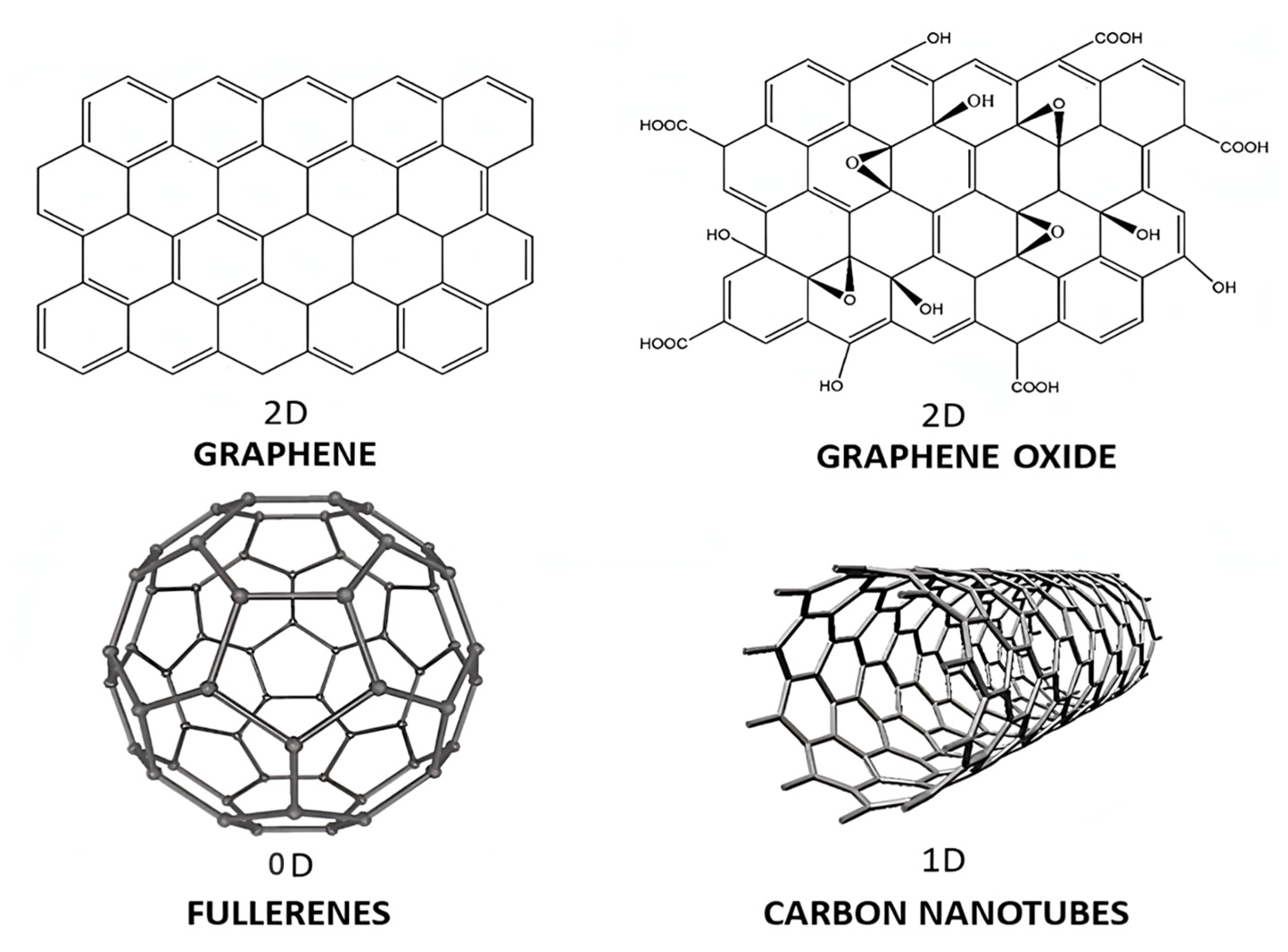
2.1. Carbon-Based Nanofillers
2.1.1. Fullerenes
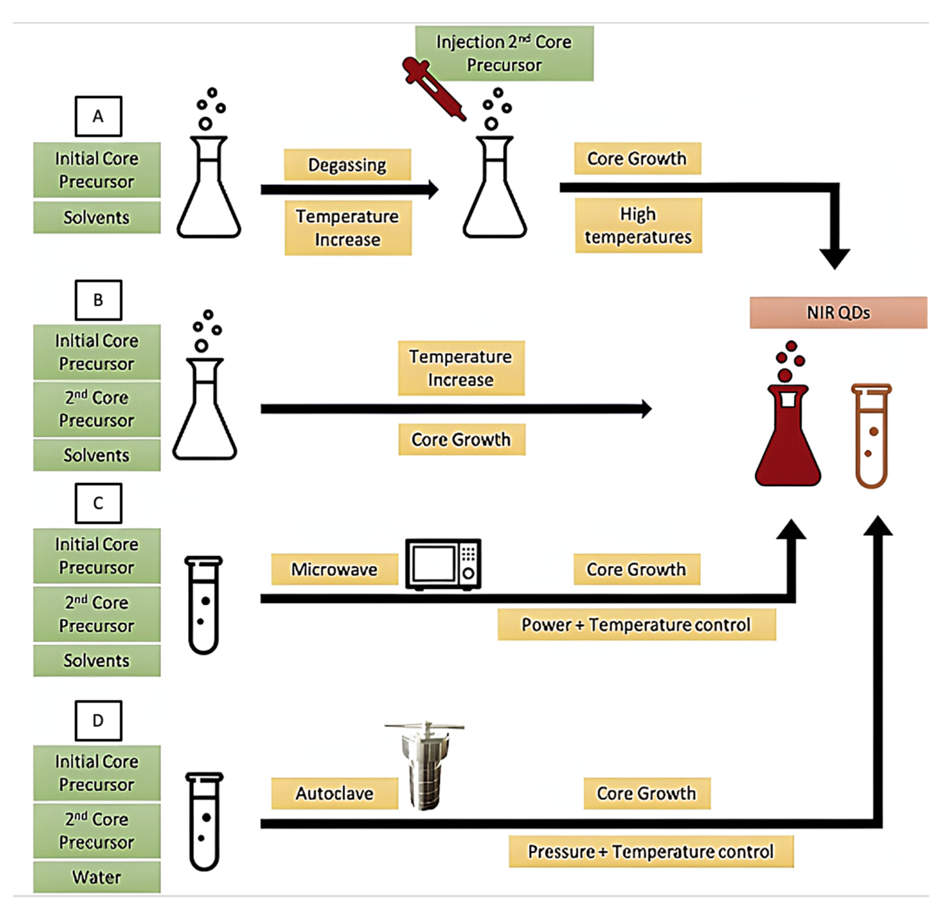
2.1.2. Quantum Dots
2.1.3. Carbon Nanotubes
2.1.4. Graphene and Its Derivatives
2.2. Inorganic Nanofillers
2.2.1. Layered Nanoclays
2.2.2. Metallic Nanoparticles
2.2.3. Metal Oxide Nanoparticles
2.3. Organic Nanofillers
2.3.1. Nanomicelles
2.3.2. Liposomes
2.3.3. Nanodendrimers
3. Machine Learning Applied to Polymeric Nanocomposites
3.1. Classification of Machine Learning
- Data acquisition: data should be collected in a systematic way from published articles, technical reports or from own experimental data. It should be noted that some data sources or published articles do not report all considered variables.
- Data preparation: After collecting the suitable data, preprocessing is carried out in terms of formatting, cleaning and sampling. Formatting provides a structure to the data which enhances its quality. Relevant materials and process variables affecting the behaviour to be modelled need to be carefully examined. Nanofiller-related parameters need to be considered, such as type, concentration, shape and size, matrix parameters including nature and concentration, the manufacturing process to fabricate the nanocomposites as well as some nanocomposite properties, such as density, thickness, porosity, etc. Some of the attributes are deleted in the cleaning step in order to keep the consistency of all recovered values and ensure data quality. Incorrect data can hinder the accuracy of ML predictive models. Erroneous data may arise during both recovering data points from the literature or entering the datapoint into the database. All entered values need to be double checked to verify that no erroneous value was included. Then, sampling is used to select a subset of the data out of a big chunk which can further be used for the training purpose [88]. Converting the raw information into certain relevant attributes which are further used as input features for the selected algorithm is a necessary step for getting accurate predictions and is commonly known as feature engineering [89]. It helps in increasing the learning accuracy along with improved comprehensibility.
- Selection of the ML method: After data preparation, the next step is to set a hypothesis function (h(x)) which maps the input parameters (x) to the output (y) and selects a suitable ML algorithm to be used (Figure 10). Based on the type of data and whether the problem is a classification or regression, an appropriate algorithm is chosen [90]. The algorithms most widely used for classification problems are K-nearest neighbour (KNN), decision trees, neural networks, naive bayes and support vector machine [91]. For problem regressions, algorithms such as linear regression, support vector regression, neural networks, Gaussian process and ensemble methods are typically applied [92].
- Training: The selected algorithm is trained with the processed data, which are split into three subsections: training, cross-validation and testing dataset. The model learns to process the information using a training dataset. A cross-validation dataset is used for parameter tuning and to prevent overfitting issues.
- Model evaluation: This is a critical part of the model development process. A model can be inaccurate despite having a very small data training error. With this aim, a test dataset is applied to assess the model’s performance, and this sets the basis for making the final predictions. Accordingly, the final model is chosen and the hypothesis function is also evaluated. Figure 10 shows the basic scheme for the initial implementation of ML.
3.2. Property Prediction, Process Optimization and Uncertainty Quantification
3.3. ML Algorithms Used in Polymer Nanocomposites
3.3.1. Neural Networks
Y = A (W × x + Bi) + B0
3.3.2. Genetic Algorithm
- The evolution of a maximum number of generations.
- Reaching a certain number of generations in which no appreciable improvement in the population is detected. After successive generations the average fitness value in the population remains constant.
- Finding a solution sufficiently close to a previously bounded optimum.
Solution Coding
- Binary coding. This can be either common binary coding or Gray’s binary coding.
- Coding with integer values, the content of the genes belongs to the set of integers .
- Coding with real values, analogous to the previous one but the variables can only take values in .
- Finite value coding, in which the variables can take only values pertaining to a limited set of values, such as a set of predefined colours or a closed set of positions on a board.
Selection of Individuals
- Selective pressure: allows the best individuals to be selected for the recombination process. It is necessary so that the search process is not random and there is a certain degree of convergence, focusing the search on promising regions.
- Diversity refers to the differences between individuals. The lack of genetic diversity causes all individuals in the population to be similar, so their offspring will be similar as well. The algorithm will progress very slowly or not at all.
- Selection by tournament: this technique was proposed by [152] and subsequently studied in [153]. Selection is performed by direct comparisons of the fitness values of individuals. A number p of individuals is randomly selected. Typically, p = 2 is used, i.e., a tournament by pairs of individuals. From each pair, the individual with the best fitness wins. This process is repeated until the selection of individuals is complete. A variant of this method is to assign a probability of success to the fittest individual in each set. In this way, the fitness value does not always win.
- Uniform state selection: was proposed by [154] for non-generational genetic algorithms, in which in each generation, only a few individuals are replaced by fitter ones. It consists of selecting the fittest individuals and subjecting them to the crossover and mutation operators. The resulting fittest offspring will replace the worst individuals in the population in the next generation.
- Proportional selection: individuals are chosen according to the contribution of their fitness value with respect to the contributions of the rest of the population. This technique was originally presented by [137] and further developed by [155]. Variants have appeared, the most widely used of which is the roulette technique.
Crossing Operator
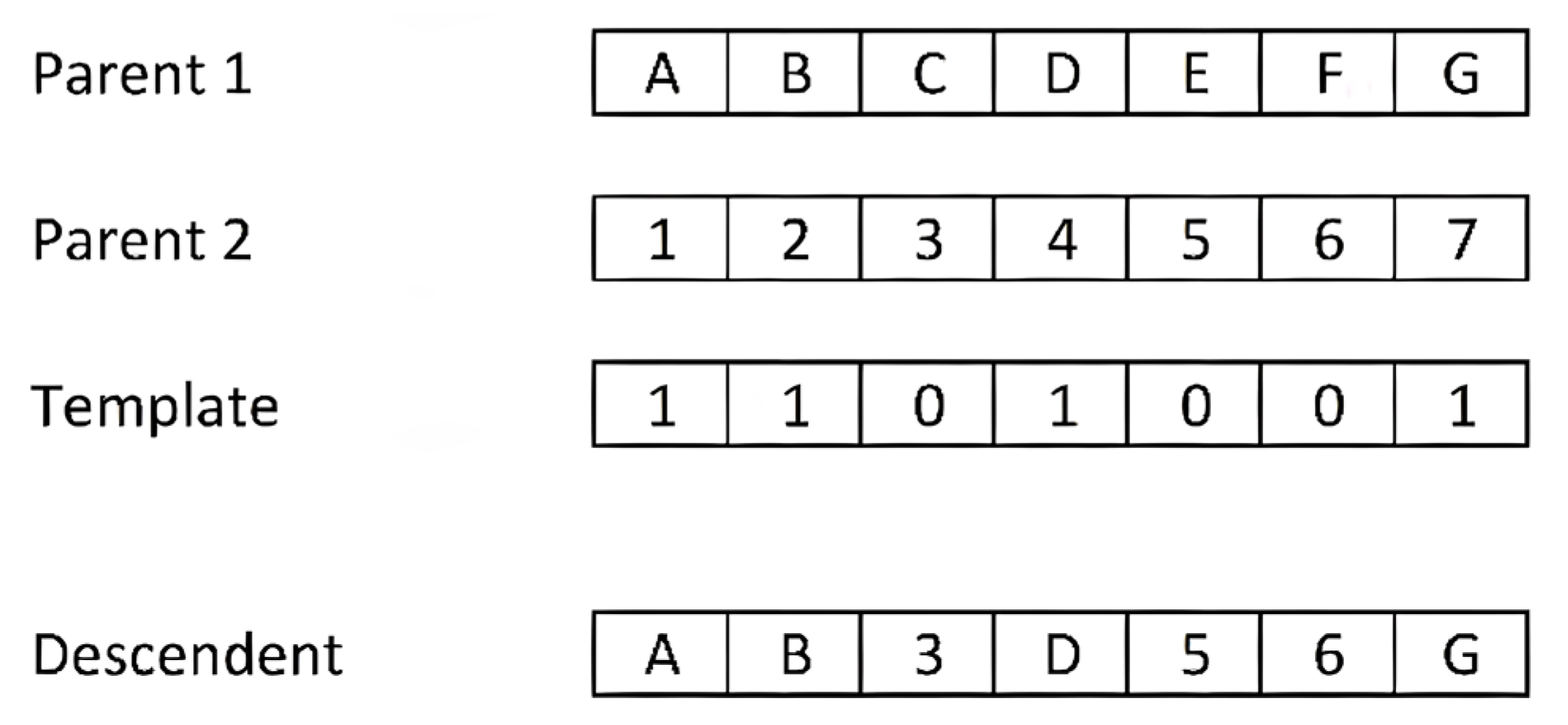
- Single point crossover: This method was proposed by [137] and is the simplest and most popular. Subsequently, several variants have emerged. It consists of sectioning both parent chromosomes at a random point, with each chromosome being subdivided into two parts. The offspring is composed of one part of each chromosome. Figure 18 shows an example of a single-point crossover. We have used letters (A–G) for the content of the first parent and numbers (1–7) for the second, with the intention of highlighting the origin of the fragments in the offspring. Both parents have a length of seven alleles, and the cut-off point is located between the fourth and fifth allele. The offspring is assembled from the initial fragment of parent 1 and the final fragment of the chromosome 2.
- Multi-point crossover: this was proposed by [156] as a generalisation of single-point crossover. It consists of fragmenting both of the parent chromosomes by N random points, thus obtaining N + 1 fragments of each. The offspring is built by alternating fragments from each parent. It has been experimentally proven that the N = 2 value gives better results than single-point cutting. This method shows a greater tendency to fragment the chromosomes in the central sections than in the areas near the ends [157].
- Uniform crossover: this can be considered as the extreme case of N-point crossover in the sense that each gene is considered a fragment of the chromosome. The offspring is formed by permuting the genes of both parents with a certain probability. In most cases a probability of 0.5 is taken, although some researchers recommend a somewhat lower probability. The assignment of the content for each gene of the offspring is performed according to a binary mask of the same length as the parent chromosomes, in which the value “1” at position i means assigning gene i of the offspring the value of the same gene of one parent, while the value “0” indicates assigning the content of gene i of the other parent. Figure 19 shows an example of a uniform crossover with a binary mask generated by applying a probability of 0.5. Therefore, the offspring receive information from both parents at 50%.
- Shuffle crossover: this is a technique that can be incorporated into the three previous types of crossovers in order to reduce the tendency to fragment chromosomes at the central sections. It consists of applying the same random permutation to both parents before the crossing operation. After the crossover operation, the reverse permutation must be applied to the offspring. In this way, the positions of the cut-off points are more evenly distributed throughout the individual.
- Partial map crossover: this operator is applied in order-based encodings (permutations) in which the value for a gene cannot be repeated in the same chromosome. The classic example for this type of coding is the Packet problem, in which each packet is represented only once in the chromosome content. This type of crossover copies part of the genetic information of one of the two parents into the offspring, with its exact sequence and in the same position. The crossover process is as follows: N cut points are applied to one of the parents and alternating fragments of the parent are transferred in their entirety to the individual offspring in a similar way to the multipoint crossover. For N = 2, the first and third fragments of the selected parent would be copied to the offspring. The remaining fragments for the offspring are filled with the values of the genes not present in the offspring and in the order of occurrence of the second parent. Figure 20 shows an example of this method with N = 2 and the cut-off points between the second and third genes, and between the fifth and sixth genes. We have chosen the parents (A B C D E F G) and their inverse (G F E D C B A) to have a simple example. The offspring chromosome takes the end fragments from the first parent, resulting in (A B - - - F G). We filled in the three free gaps with the genes from the second parent in order of appearance, if not already present. In the example, the first two genes of the second parent (G F) are not considered because they are already included in the offspring; only (E D C) is filled in.
Mutation Operator
- The exploration of new areas in the space of solutions close to “quality solutions” already studied.
- Ensures diversity in the population to avoid premature convergence of the algorithm.
- In case of premature convergence to a local optimum, the algorithm can be free from that local maximum/minimum.
- Swap mutation involves exchanging the values of randomly selected genes.
- Adjacent genes swap mutation selects two consecutive genes on the chromosome and reverses their order.
- In inversion mutation, two random positions on the chromosome are chosen and the gene values are swapped between them. Suppose the positions are i and j. The in-terchange operation exchanges the value of gene i with j and vice versa, exchanging genes (i + 1) and (j − 1), (i + 2) with (j − 2) and so on until the interval [i–j] is covered, the last genes exchanged being (i + n) and (j − n), with n = (j − i + 1)/2.
- In shift mutation, a set of consecutive genes to be altered and a direction of displacement (to the right or to the left) is determined. The process consists of each gene in the interval moving to occupy the immediate position until the last gene affected is made to correspond to the first position of the same group of genes. The effect is that the values of all affected genes are shifted one position on the chromosome.
Local Search
- Extending the size of the neighbourhood.
- Limiting the number of search iterations.
- Repeating the search algorithm with different starting solutions.
3.3.3. Gaussian Process
4. Conclusions and Future Outlook
Author Contributions
Funding
Institutional Review Board Statement
Informed Consent Statement
Data Availability Statement
Conflicts of Interest
References
- Sahoo, N.G.; Rana, S.; Cho, J.W.; Li, L.; Chan, S.H. Polymer nanocomposites based on functionalized carbon nanotubes. Prog. Polym. Sci. 2010, 35, 837–867. [Google Scholar] [CrossRef]
- Díez-Pascual, A.M. Carbon-Based Polymer Nanocomposites for High-Performance Applications II. Polymers 2022, 14, 870. [Google Scholar] [CrossRef] [PubMed]
- Kickelbick, G. Concepts for the incorporation of inorganic building blocks into organic polymers on a nanoscale. Prog. Polym. Sci. 2003, 28, 83–114. [Google Scholar] [CrossRef]
- Díez-Pascual, A.M. Chemical Functionalization of Carbon Nanotubes with Polymers: A Brief Overview. Macromol 2021, 1, 64–83. [Google Scholar] [CrossRef]
- Díez-Pascual, A.M. Surface Engineering of Nanomaterials with Polymers, Biomolecules, and Small Ligands for Nanomedicine. Materials 2022, 15, 3251. [Google Scholar] [CrossRef]
- Díez-Pascual, A.M.; Naffakh, M.; Marco, C.; Ellis, G.; Gomez-Fatou, M.A. High-performance nanocomposites based on polyetherketones. Prog. Mater. Sci. 2012, 57, 1106–1190. [Google Scholar] [CrossRef]
- Nanomaterials definition matters. Nat. Nanotechnol. 2019, 14, 193. [CrossRef]
- Khan, I.; Saeed, K.; Khan, I. Nanoparticles: Properties, applications and toxicities. Arab. J. Chem. 2019, 12, 908–931. [Google Scholar] [CrossRef]
- Pokropivny, V.V.; Skorokhod, V.V. Classification of nanostructures by dimensionality and concept of surface forms engineering in nanomaterial science. Mater. Sci. Eng. C 2007, 27, 990–993. [Google Scholar] [CrossRef]
- Müller, K.; Bugnicourt, E.; Latorre, M.; Jorda, M.; Echegoyen Sanz, Y.; Lagaron, J.M.; Miesbauer, O.; Bianchin, A.; Hankin, S.; Bölz, U.; et al. Review on the processing and properties of polymer nanocomposites and nanocoatings and their applications in the packaging, automotive and solar energy fields. Nanomaterials 2017, 7, 74. [Google Scholar] [CrossRef] [Green Version]
- Bitinis, N.; Hernandez, M.; Verdejo, R.; Kenny, J.M.; Lopez-Manchado, M.A. Recent Advances in Clay/Polymer Nanocomposites. Adv. Mater. 2011, 23, 5229–5236. [Google Scholar] [CrossRef] [PubMed]
- Luceño-Sánchez, J.A.; Charas, A.; Díez-Pascual, A.M. Effect of HDI-Modified GO on the Thermoelectric Performance of Poly(3,4-ethylenedioxythiophene):Poly(Styrenesulfonate) Nanocomposite Films. Polymers 2021, 13, 1503. [Google Scholar] [CrossRef] [PubMed]
- Díez-Pascual, A.M. Effect of Graphene Oxide on the Properties of Poly(3-Hydroxybutyrate-co-3-Hydroxyhexanoate). Polymers 2021, 13, 2233. [Google Scholar] [CrossRef]
- Alexandre, M.; Dubois, P. Polymer-layered silicate nanocomposites: Preparation, properties and uses of a new class of materials. Mater. Sci. Eng. R Rep. Rev. J. 2000, 28, 1–63. [Google Scholar] [CrossRef]
- Díez-Pascual, A.M. Nanoparticle Reinforced Polymers. Polymers 2019, 11, 625. [Google Scholar] [CrossRef]
- Díez-Pascual, A.M. Biopolymer Composites: Synthesis, Properties, and Applications. Int. J. Mol. Sci. 2022, 23, 2257. [Google Scholar] [CrossRef]
- Meijer, G.; Ellyin, F.; Xia, Z. Aspects of residual thermal stress/strain in particle reinforced metal matrix composites. Composites Part B Eng. 2000, 31, 29–37. [Google Scholar] [CrossRef]
- Haque, A.; Ramasetty, A. Theoretical study of stress transfer in carbon nanotube reinforced polymer matrix composites. Compos. Struct. 2005, 71, 68–77. [Google Scholar] [CrossRef]
- McCartney, L.N. New Theoretical Model of Stress Transfer Between Fibre and Matrix in a Uniaxially Fibre-Reinforced Composite. Proc. R. Soc. Lond. A 1989, 425, 215–244. [Google Scholar]
- Rossman, T.; Kushvaha, V.; Dragomir-Daescu, D. QCT/FEA predictions of femoral stiffness are strongly affected by boundary condition modeling. Comput. Methods Biomech. Biomed. Eng. 2016, 19, 208–216. [Google Scholar] [CrossRef]
- Frankland, S.J.V.; Harik, V.M.; Odegard, G.M.; Brenner, D.W.; Gates, T.S. The stress–strain behavior of polymer–nanotube composites from molecular dynamics simulation. Compos. Sci. Technol. 2003, 63, 1655–1661. [Google Scholar] [CrossRef]
- Li, Y.; Wang, S.; Wang, Q.; Xing, M. Enhancement of fracture properties of polymer composites reinforced by carbon nanotubes: A molecular dynamics study. Carbon 2018, 129, 504–509. [Google Scholar] [CrossRef]
- Gu, G.X.; Chen, C.; Richmond, D.J.; Buehler, M.J. Bioinspired hierarchical composite design using machine learning: Simulation, additive manufacturing, and experiment. Mater. Horiz. 2018, 5, 939–945. [Google Scholar] [CrossRef]
- Doan Tran, H.; Kim, C.; Chen, L.; Chandrasekaran, A.; Batra, R.; Venkatram, S.; Kamal, D.; Lightstone, J.P.; Gurnani, R.; Shetty, P.; et al. Machine-learning predictions of polymer properties with Polymer Genome. J. Appl. Phys. 2020, 128, 171104. [Google Scholar] [CrossRef]
- Zhou, T.; Song, Z.; Sundmacher, K. Big Data Creates New Opportunities for Materials Research: A Review on Methods and Applications of Machine Learning for Materials Design. Engineering 2019, 5, 981–1192. [Google Scholar] [CrossRef]
- Butler, K.T.; Davies, D.W.; Cartwright, H.; Isayev, O.; Walsh, A. Machine learning for molecular and materials science. Nature 2018, 559, 547–555. [Google Scholar] [CrossRef]
- Kumar, J.N.; Li, Q.; Jun, Y. Challenges and opportunities of polymer design with machine learning and high throughput experimentation. MRS Commun. 2019, 9, 537–544. [Google Scholar] [CrossRef]
- Jackson, N.E.; Webb, M.A.; de Pablo, J.J. Recent advances in machine learning towards multiscale soft materials design. Curr. Opin. Chem. Eng. 2019, 23, 106–114. [Google Scholar] [CrossRef]
- Díez-Pascual, A.M. Carbon-Based Nanomaterials. Int. J. Mol. Sci. 2021, 22, 7726. [Google Scholar] [CrossRef]
- Díez-Pascual, A.M.; Díez-Vicente, A.L. Poly(propylene fumarate)/Polyethylene Glycol-Modified Graphene Oxide Nanocomposites for Tissue Engineering. ACS Appl. Mater. Interfaces 2016, 8, 17902–17914. [Google Scholar] [CrossRef]
- Kroto, H.W.; Heath, J.R.; O’Brien, S.C.; Curl, R.F.; Smalley, R.E. C60: Buckminsterfullerene. Nature 1985, 318, 162–163. [Google Scholar] [CrossRef]
- Kroto, H.W. C60: Buckminsterfullerene, The Celestial Sphere that Fell to Earth. Angew. Chem. (Int. Ed.) 1992, 31, 111–129. [Google Scholar] [CrossRef]
- Yadav, J. Fullerene: Properties, synthesis and application. Res. Rev. J. Phys. 2018, 6, 1–6. [Google Scholar]
- Murray, C.B.; Kagan, C.R.; Bawendi, M.G. Synthesis and characterization of monodisperse nanocrystals and close-packed nanocrystal assemblies. Annu. Rev. Mater. Res. 2000, 30, 547–610. [Google Scholar] [CrossRef]
- Xu, X.; Ray, R.; Gu, Y.; Ploehn, H.J.; Gearheart, L.; Raker, K.; Scrivens, W.A. Electrophoretic Analysis and Purification of Fluorescent Single-Walled Carbon Nanotube Fragments. J. Am. Chem. Soc. 2004, 126, 12736–12737. [Google Scholar] [CrossRef]
- Jaiswal, J.K.; Goldman, E.R.; Mattoussi, H.; Simon, S.M. Use of quantum dots for live cell imaging. Nat. Methods 2004, 1, 6. [Google Scholar] [CrossRef]
- Zajac, A.; Song, D.; Qian, W.; Zhukov, T. Protein microarrays and quantum dot probes for early cancer detection. Colloids Surf. B Biointerfaces 2007, 58, 309–314. [Google Scholar] [CrossRef]
- Gil, H.M.; Price, T.W.; Chelani, K.; Bouillard, J.G.; Calaminus, S.D.J.; Stasiuk, G.J. NIR-quantum dots in biomedical imaging and their future. iScience 2021, 24, 102189. [Google Scholar] [CrossRef]
- Sun, J.; Wang, W.; Yue, Q. Review on Microwave-Matter Interaction Fundamentals and Efficient Microwave-Associated Heating Strategies. Materials 2016, 9, 231. [Google Scholar] [CrossRef]
- Iijima, S. Helical microtubules of graphitic carbon. Nature 1991, 354, 56–58. [Google Scholar] [CrossRef]
- Saito, R.; Fujita, M.; Dresselhaus, G.; Dresselhaus, M.S. Electronic structure of chiral graphene tubules. Appl. Phys. Lett. 1992, 60, 2204–2206. [Google Scholar] [CrossRef]
- Yu, M.; Files, B.; Arepalli, S.; Ruoff, R. Tensile Loading of Ropes of Single Wall Carbon Nanotubes and their Mechanical Properties. Phys. Rev. Lett. 2000, 84, 5552–5555. [Google Scholar] [CrossRef] [PubMed] [Green Version]
- Bom, D.; Andrews, R.; Jacques, D.; Anthony, J.; Chen, B.; Meier, M.S.; Selegue, J.P. Thermogravimetric Analysis of the Oxidation of Multiwalled Carbon Nanotubes: Evidence for the Role of Defect Sites in Carbon Nanotube Chemistry. Nano Lett. 2002, 2, 615–619. [Google Scholar] [CrossRef]
- Hirsch, A. Functionalization of Single-Walled Carbon Nanotubes. Angew. Chem. (Int. Ed.) 2002, 41, 1853–1859. [Google Scholar] [CrossRef]
- Díez-Pascual, A.M.; Naffakh, M.; Gómez, M.A.; Marco, C.; Ellis, G.; Martínez, M.T.; Ansón, A.; González-Domínguez, J.M.; Martínez-Rubi, Y.; Simard, B. Development and characterization of PEEK/carbon nanotube composites. Carbon 2009, 47, 3079–3090. [Google Scholar] [CrossRef]
- Díez-Pascual, A.M.; Naffakh, M.; Gómez, M.A.; Marco, C.; Ellis, G.; González-Domínguez, J.M.; Ansón, A.; Martínez, M.T.; Martínez-Rubi, Y.; Simard, B.; et al. The influence of a compatibilizer on the thermal and dynamic mechanical properties of PEEK/carbon nanotube composites. Nanotechnology 2009, 20, 315707. [Google Scholar] [CrossRef]
- Harris, P.J.F.; Hirsch, A.; Backes, C. Carbon Nanotubes Science: Synthesis, Properties and Applications; Cambridge University Press: Cambridge, UK, 2009; Volume 102, pp. 210–230. [Google Scholar]
- Novoselov, K.S.; Geim, A.K.; Morozov, S.V.; Jiang, D.; Zhang, Y.; Dubonos, S.V.; Grigorieva, I.V.; Firsov, A.A. Electric Field Effect in Atomically Thin Carbon Films. Science 2004, 306, 666–669. [Google Scholar] [CrossRef]
- Geim, A.K.; Novoselov, K.S. The rise of graphene. Nat. Mater. 2007, 6, 183–191. [Google Scholar] [CrossRef]
- Balandin, A.A.; Ghosh, S.; Bao, W.; Calizo, I.; Teweldebrhan, D.; Miao, F.; Lau, C.N. Superior Thermal Conductivity of Single-Layer Graphene. Nano Lett. 2008, 8, 902–907. [Google Scholar] [CrossRef]
- Diez-Pascual, A.M.; Gomez-Fatou, M.A.; Ania, F.; Flores, A. Nanoindentation in polymer nanocomposites. Prog. Mater. Sci. 2015, 67, 1–94. [Google Scholar] [CrossRef]
- Díez-Pascual, A.M.; Luceño Sánchez, J.A.; Peña Capilla, R.; García Díaz, P. Recent Developments in Graphene/Polymer Nanocomposites for Application in Polymer Solar Cells. Polymers 2018, 10, 217. [Google Scholar] [CrossRef] [PubMed]
- Díez-Pascual, A.M. Graphene-based polymer composites: Recent advances. Polymers 2022, 14, 2102. [Google Scholar] [CrossRef]
- Morales Narváez, E.; Baptista Pires, L.M.; Zamora Gálvez, A.; Merkoçi, A. Graphene-Based Biosensors: Going Simple. Adv. Mater. 2017, 29, 1604905. [Google Scholar] [CrossRef]
- Mateos, R.; Vera, S.; Valiente, M.; Díez-Pascual, A.M.; San Andrés, M.P. Comparison of Anionic, Cationic and Nonionic Surfactants as Dispersing Agents for Graphene Based on the Fluorescence of Riboflavin. Nanomaterials 2017, 7, 403. [Google Scholar] [CrossRef]
- Lotya, M.; Hernandez, Y.; King, P.J.; Smith, R.J.; Nicolosi, V.; Karlsson, L.S.; Blighe, F.M.; De, S.; Wang, Z.; McGovern, I.T.; et al. Liquid Phase Production of Graphene by Exfoliation of Graphite in Surfactant/Water Solutions. J. Am. Chem. Soc. 2009, 131, 3611–3620. [Google Scholar] [CrossRef] [PubMed]
- Sainz-Urruela, C.; Vera-López, S.; San Andrés, M.P.; Díez-Pascual, A.M. Graphene Oxides Derivatives Prepared by an Electrochemical Approach: Correlation between Structure and Properties. Nanomaterials 2020, 10, 2532. [Google Scholar] [CrossRef] [PubMed]
- Díez-Pascual, A.M.; Sainz-Urruela, C.; Vallés, C.; Vera-López, S.; Andrés, M.P.S. Tailorable Synthesis of Highly Oxidized Graphene Oxides via an Environmentally-Friendly Electrochemical Process. Nanomaterials 2020, 10, 239. [Google Scholar] [CrossRef]
- Li, X.; Cai, W.; An, J.; Kim, S.; Nah, J.; Yang, D.; Piner, R.; Velamakanni, A.; Jung, I.; Tutuc, E.; et al. Large-Area Synthesis of High-Quality and Uniform Graphene Films on Copper Foils. Science 2009, 324, 1312–1314. [Google Scholar] [CrossRef]
- Zaaba, N.I.; Foo, K.L.; Hashim, U.; Tan, S.J.; Liu, W.; Voon, C.H. Synthesis of Graphene Oxide using Modified Hummers Method: Solvent Influence. Procedia Eng. 2017, 184, 469–477. [Google Scholar] [CrossRef]
- Luceño-Sánchez, J.A.; Maties, G.; Gonzalez-Arellano, C.; Diez-Pascual, A.M. Synthesis and Characterization of Graphene Oxide Derivatives via Functionalization Reaction with Hexamethylene Diisocyanate. Nanomaterials 2018, 8, 870. [Google Scholar] [CrossRef]
- Dua, V.; Surwade, S.P.; Ammu, S.; Agnihotra, S.R.; Jain, S.; Roberts, K.E.; Park, S.; Ruoff, R.S.; Manohar, S.K. All-Organic Vapor Sensor Using Inkjet-Printed Reduced Graphene Oxide. Angew. Chem. (Int. Ed.) 2010, 49, 2154–2157. [Google Scholar] [CrossRef] [PubMed]
- Kotal, M.; Bhowmick, A.K. Polymer nanocomposites from modified clays: Recent advances and challenges. Prog. Polym. Sci. 2015, 51, 127–187. [Google Scholar] [CrossRef] [Green Version]
- Zaïri, F.; Gloaguen, J.M.; Naït-Abdelaziz, M.; Mesbah, A.; Lefebvre, J.M. Study of the effect of size and clay structural parameters on the yield and post-yield response of polymer/clay nanocomposites via a multiscale micromechanical modelling. Acta Mater. 2011, 59, 3851–3863. [Google Scholar] [CrossRef]
- Schadler, L.S. Polymer-Based and Polymer-Filled Nanocomposites. In Nanocomposite Science and Technology; Wiley-VCH Verlag GmbH & Co. KGaA: Weinheim, Germany, 2003; pp. 77–153. [Google Scholar]
- Ray, S.S. Recent Trends and Future Outlooks in the Field of Clay-Containing Polymer Nanocomposites. Macromol. Chem. Phys. 2014, 215, 1162–1179. [Google Scholar] [CrossRef]
- Daruich De Souza, C.; Ribeiro Nogueira, B.; Rostelato, M.E.C.M. Review of the methodologies used in the synthesis gold nanoparticles by chemical reduction. J. Alloys Compd. 2019, 798, 714–740. [Google Scholar] [CrossRef]
- Fahmy, H.M.; El-Feky, A.S.; Abd El-Daim, T.M.; Abd El-Hameed, M.M.; Gomaa, D.A.; Hamad, A.M.; Elfky, A.A.; Elkomy, Y.H.; Farouk, N.A. Eco-Friendly Methods of Gold Nanoparticles Synthesis. Nanosci. Nanotechnol.-Asia 2019, 9, 311–328. [Google Scholar] [CrossRef]
- Vanlalveni, C.; Lallianrawna, S.; Biswas, A.; Selvaraj, M.; Changmai, B.; Rokhum, S.L. Green synthesis of silver nanoparticles using plant extracts and their antimicrobial activities: A review of recent literature. RSC Adv. 2021, 11, 284–2837. [Google Scholar] [CrossRef]
- Hamad, A.; Khashan, K.S.; Hadi, A. Silver Nanoparticles and Silver Ions as Potential Antibacterial Agents. J. Inorg. Organomet. Polym. 2020, 30, 4811–4828. [Google Scholar] [CrossRef]
- Parveen, F.; Sannakki, B.; Mandke, M.V.; Pathan, H.M. Copper nanoparticles: Synthesis methods and its light harvesting performance. Sol. Energy Mater. Sol. Cells 2016, 144, 371–382. [Google Scholar] [CrossRef]
- Díez-Pascual, A.M.; Díez-Vicente, A.L. Epoxidized Soybean Oil/ZnO Biocomposites for Soft Tissue Applications: Preparation and Characterization. ACS Appl. Mater. Interfaces 2014, 6, 17277–17288. [Google Scholar] [CrossRef]
- Waghmode, M.S.; Gunjal, A.B.; Mulla, J.A.; Patil, N.N.; Nawani, N.N. Studies on the titanium dioxide nanoparticles: Biosynthesis, applications and remediation. SN Appl. Sci 2019, 1, 310. [Google Scholar] [CrossRef]
- Díez-Pascual, A.M.; Díez-Vicente, A.L. Development of linseed oil-TiO2 green nanocomposites as antimicrobial coatings. J. Mater. Chem. B Mater. Biol. Med. 2015, 3, 4458–4471. [Google Scholar] [CrossRef] [PubMed]
- Samrot, A.V.; Sahithya, C.S.; Selvarani, A.J.; Purayil, S.K.; Ponnaiah, P. A review on synthesis, characterization and potential biological applications of superparamagnetic iron oxide nanoparticles. Curr. Res. Green Sustain. Chem. 2021, 4, 100042. [Google Scholar] [CrossRef]
- Vadlapudi, A.D.; Mitra, A.K. Nanomicelles: An emerging platform for drug delivery to the eye. Ther. Deliv. 2013, 4, 1–3. [Google Scholar] [CrossRef] [PubMed]
- Akbarzadeh, A.; Rezaei-Sadabady, R.; Davaran, S.; Joo, S.W.; Zarghami, N.; Hanifehpour, Y.; Samiei, M.; Kouhi, M.; Nejati-Koshki, K. Liposome: Classification, preparation, and applications. Nanoscale Res. Lett. 2013, 8, 102. [Google Scholar] [CrossRef] [PubMed]
- Vögtle, F.; Richardt, G.; Werner, N. Dendrimer Chemistry Concepts, Syntheses, Properties, Applications; Wiley-VCH: Weinheim, Germany, 2009. [Google Scholar]
- Turing, A.M. Computing Machinery and Intelligence. Mind 1950, 59, 433–460. [Google Scholar] [CrossRef]
- Schmidt, J.; Marques, M.R.G.; Botti, S.; Marques, M.A.L. Recent advances and applications of machine learning in solid-state materials science. Npj Comput. Mater. 2019, 5, 83. [Google Scholar] [CrossRef]
- Webb, S. Deep learning for biology. Nature 2018, 554, 555–557. [Google Scholar] [CrossRef]
- Xu, C.; Jackson, S.A. Machine learning and complex biological data. Genome Biol. 2019, 20, 76. [Google Scholar] [CrossRef]
- Liu, Y.; Niu, C.; Wang, Z.; Gan, Y.; Zhu, Y.; Sun, S.; Shen, T. Machine learning in materials genome initiative: A review. J. Mater. Sci. Technol. 2020, 57, 113–122. [Google Scholar] [CrossRef]
- Riedmiller, M. Advanced supervised learning in multi-layer perceptrons—From backpropagation to adaptive learning algorithms. Comput. Stand. Interfaces 1994, 16, 265–278. [Google Scholar] [CrossRef]
- Zhang, M.; Zhou, Z. A Review on Multi-Label Learning Algorithms. TKDE 2014, 26, 1819–1837. [Google Scholar] [CrossRef]
- Barlow, H.B. Unsupervised Learning; MIT Press: Cambridge, MA, USA, 1989; Volume 1, pp. 295–311. [Google Scholar]
- Figueiredo, M.A.T.; Jain, A.K. Unsupervised learning of finite mixture models. TPAMI 2002, 24, 381–396. [Google Scholar] [CrossRef]
- Xu, Y.; Goodacre, R. On Splitting Training and Validation Set: A Comparative Study of Cross-Validation, Bootstrap and Systematic Sampling for Estimating the Generalization Performance of Supervised Learning. J. Anal. Test 2018, 2, 249–262. [Google Scholar] [CrossRef] [PubMed]
- Langley, P. Selection of Relevant Features in Machine Learning. In Proceedings of the AAAI Fall Symposium on Relevance, New Orleans, LA, USA, 4–6 November 1994. [Google Scholar]
- Yu, L.; Liu, H. Eficient Feature Selection Via Analysis of Relevance and Redundancy. J. Mach. Learn. Res. 2004, 5, 1205–1224. [Google Scholar]
- Sharma, S.; Agrawal, J.; Sharma, S. Classification Through Machine Learning Technique: C4. 5 Algorithm based on Various Entropies. Int. J. Comput. Appl. 2013, 82, 28–32. [Google Scholar] [CrossRef]
- PARDALOS, P.M.; XUE, G. Algorithms for a Class of Isotonic Regression Problems. Algorithmica 1999, 23, 211–222. [Google Scholar] [CrossRef]
- Francisco, M.; Revollar, S.; Vega, P.; Lamanna, R. A comparative study of deterministic and stochastic optimization methods for integrated design of processes. IFAC Proc. Vol. 2005, 38, 335–340. [Google Scholar] [CrossRef]
- Sun, S. A review of deterministic approximate inference techniques for Bayesian machine learning. Neural Comput. Applic. 2013, 23, 2039–2050. [Google Scholar] [CrossRef]
- Pedro, H.T.C.; Coimbra, C.F.M.; David, M.; Lauret, P. Assessment of machine learning techniques for deterministic and probabilistic intra-hour solar forecasts. Renew. Energy 2018, 123, 191–203. [Google Scholar] [CrossRef]
- Chatterjee, T.; Chakraborty, S.; Chowdhury, R. A Critical Review of Surrogate Assisted Robust Design Optimization. Arch. Computat. Methods Eng. 2017, 26, 245–274. [Google Scholar] [CrossRef]
- Sarkar, S.; Vinay, S.; Raj, R.; Maiti, J.; Mitra, P. Application of optimized machine learning techniques for prediction of occupational accidents. Comput. Oper. Res. 2019, 106, 210–224. [Google Scholar] [CrossRef]
- Kalita, K.; Mukhopadhyay, T.; Dey, P.; Haldar, S. Genetic programming-assisted multi-scale optimization for multi-objective dynamic performance of laminated composites: The advantage of more elementary-level analyses. Neural Comput. Applic. 2019, 32, 7969–7993. [Google Scholar] [CrossRef]
- Salah, L.S.; Chouai, M.; Danlée, Y.; Huynen, I.; Ouslimani, N. Simulation and Optimization of Electromagnetic Absorption of Polycarbonate/CNT Composites Using Machine Learning. Micromachines 2020, 11, 778. [Google Scholar] [CrossRef]
- Khanam, P.N.; AlMaadeed, M.; AlMaadeed, S.; Kunhoth, S.; Ouederni, M.; Sun, D.; Hamilton, A.; Jones, E.H.; Mayoral, B. Optimization and Prediction of Mechanical and Thermal Properties of Graphene/LLDPE Nanocomposites by Using Artificial Neural Networks. Int. J. Polym. Sci. 2016, 2016, 1–15. [Google Scholar] [CrossRef]
- Zakaulla, M.; Pasha, Y.; Siddalingappa, S.K. Prediction of mechanical properties for polyetheretherketone composite reinforced with graphene and titanium powder using artificial neural network. Mater. Today Proc. 2022, 49, 1268–1274. [Google Scholar] [CrossRef]
- Yusoff, N.I.M.; Ibrahim Alhamali, D.; Ibrahim, A.N.H.; Rosyidi, S.A.P.; Abdul Hassan, N. Engineering characteristics of nanosilica/polymer-modified bitumen and predicting their rheological properties using multilayer perceptron neural network model. Constr. Build. Mater. 2019, 204, 781–799. [Google Scholar] [CrossRef]
- Kosicka, E.; Krzyzak, A.; Dorobek, M.; Borowiec, M. Prediction of Selected Mechanical Properties of Polymer Composites with Alumina Modifiers. Materials 2022, 15, 882. [Google Scholar] [CrossRef]
- Karsh, P.K.; Mukhopadhyay, T.; Dey, S. Stochastic low-velocity impact on functionally graded plates: Probabilistic and non-probabilistic uncertainty quantification. Compos. Part B Eng. 2019, 159, 461–480. [Google Scholar] [CrossRef]
- Hammer, B.; Villmann, T. How to process uncertainty in machine learning. In Proceedings of the European Symposium on Artificial Neural Networks, Bruges, Belgium, 25–27 April 2007. [Google Scholar]
- Doh, J.; Park, S.; Yang, Q.; Raghavan, N. Uncertainty quantification of percolating electrical conductance for wavy carbon nanotube-filled polymer nanocomposites using Bayesian inference. Carbon 2021, 172, 308–323. [Google Scholar] [CrossRef]
- Anderson, D.; McNeill, G. Artificial Neural Networks Technology; Kaman Sciences Corporation: Utica, NJ, USA, 1992. [Google Scholar]
- Wanas, N.; Auda, G.; Kamel, M.S.; Karray, F. On the Optimal Number of Hidden Nodes in a Neural Network. In Proceedings of the IEEE Canadian Conference on Electrical and Computer Engineering, Waterloo, ON, Canada, 25–28 May 1998; IEEE: Piscataway, NJ, USA, 1998; Volume 2, pp. 918–921. [Google Scholar]
- Aleksander, I.; Morton, H. Anœ Introduction to Neural Computing; Chapman and Hall: London, UK, 1990. [Google Scholar]
- Lynch, M.; Patel, H.; Abrahamse, A.; Rupa Rajendran, A.; Medsker, L. Neural Network Applications in Physics. In Proceedings of the International Joint Conference on Neural Networks, Washington, DC, USA, 15–19 July 2001; IEEE: Piscataway, NJ, USA, 2001; Volume 3, pp. 2054–2058. [Google Scholar]
- Moradkhani, H.; Hsu, K.; Gupta, H.V.; Sorooshian, S. Improved streamflow forecasting using self-organizing radial basis function artificial neural networks. J. Hydrol. 2004, 295, 246–262. [Google Scholar] [CrossRef]
- Matos, M.A.S.; Pinho, S.T.; Tagarielli, V.L. Application of machine learning to predict the multiaxial strain-sensing response of CNT-polymer composites. Carbon 2019, 146, 265–275. [Google Scholar] [CrossRef]
- Hamdia, K.M.; Lahmer, T.; Nguyen-Thoi, T.; Rabczuk, T. Predicting the fracture toughness of PNCs: A stochastic approach based on ANN and ANFIS. Comput. Mater. Sci. 2015, 102, 304–313. [Google Scholar] [CrossRef]
- Sharma, A.; Anand Kumar, S.; Kushvaha, V. Effect of aspect ratio on dynamic fracture toughness of particulate polymer composite using artificial neural network. Eng. Fract. Mech. 2020, 228, 106907. [Google Scholar] [CrossRef]
- Zhu, J.; Shi, Y.; Feng, X.; Wang, H.; Lu, X. Prediction on tribological properties of carbon fiber and TiO2 synergistic reinforced polytetrafluoroethylene composites with artificial neural networks. Mater. Eng. 2009, 30, 1042–1049. [Google Scholar] [CrossRef]
- Mahalingam, S.; Gopalan, V.; Velivela, H.; Pragasam, V.; Prabhakaran, P.; Suthenthiraveerappa, V. Studies on Shear Strength of CNT/Coir Fibre/Fly Ash Reinforced Epoxy Polymer Composites. Emerg. Mater. Res. 2020, 9, 78–88. [Google Scholar] [CrossRef]
- Adesina, O.T.; Jamiru, T.; Daniyan, I.A.; Sadiku, E.R.; Ogunbiyi, O.F.; Adesina, O.S.; Beneke, L.W. Mechanical property prediction of SPS processed GNP/PLA polymer nanocomposite using artificial neural network. Cogent Eng. 2020, 7, 1720894. [Google Scholar] [CrossRef]
- Omari, M.A.; Almagableh, A.; Sevostianov, I.; Ashhab, M.S.; Yaseen, A.B. Modeling of the viscoelastic properties of thermoset vinyl ester nanocomposite using artificial neural network. Int. J. Eng. Sci. 2020, 150, 103242. [Google Scholar] [CrossRef]
- Yan, S.; Zou, X.; Ilkhani, M.; Jones, A. An efficient multiscale surrogate modelling framework for composite materials considering progressive damage based on artificial neural networks. Compos. Part B Eng. 2020, 194, 108014. [Google Scholar] [CrossRef]
- Ciaburro, G.; Iannace, G.; Passaro, J.; Bifulco, A.; Marano, A.D.; Guida, M.; Marulo, F.; Branda, F. Artificial neural network-based models for predicting the sound absorption coefficient of electrospun poly(vinyl pyrrolidone)/silica composite. Appl. Acoust. 2020, 169, 107472. [Google Scholar] [CrossRef]
- Zakaulla, M.; Parveen, F.; Amreen; Harish; Ahmad, N. Artificial neural network based prediction on tribological properties of polycarbonate composites reinforced with graphene and boron carbide particle. Mater. Today Proc. 2020, 26, 296–304. [Google Scholar] [CrossRef]
- Matos, M.A.S.; Pinho, S.T.; Tagarielli, V.L. Predictions of the electrical conductivity of composites of polymers and carbon nanotubes by an artificial neural network. Scr. Mater. 2019, 166, 117–121. [Google Scholar] [CrossRef]
- Wang, Y.; Zhang, M.; Lin, A.; Iyer, A.; Prasad, A.S.; Li, X.; Zhang, Y.; Schadler, L.S.; Chen, W.; Brinson, L.C. Mining structure-property relationships in polymer nanocomposites using data driven finite element analysis and multi-task convolutional neural networks. Mol. Syst. Des. Eng. 2020, 5, 962–975. [Google Scholar] [CrossRef]
- Lu, X.; Giovanis, D.G.; Yvonnet, J.; Papadopoulos, V.; Detrez, F.; Bai, J. A data-driven computational homogenization method based on neural networks for the nonlinear anisotropic electrical response of graphene/polymer nanocomposites. Comput Mech 2018, 64, 307–321. [Google Scholar] [CrossRef]
- Farahbakhsh, J.; Delnavaz, M.; Vatanpour, V. Simulation and characterization of novel reverse osmosis membrane prepared by blending polypyrrole coated multiwalled carbon nanotubes for brackish water desalination and antifouling properties using artificial neural networks. J. Membr. Sci. 2019, 581, 123–138. [Google Scholar] [CrossRef]
- Ataeefard, M.; Mohammadi, Y.; Saeb, M.R. Intelligently Synthesized In Situ Suspension Carbon Black/Styrene/Butylacrylate Composites: Using Artificial Neural Networks towards Printing Inks with Well-Controlled Properties. Polym. Sci. Ser. A 2019, 61, 667–680. [Google Scholar] [CrossRef]
- Özcanli, Y.; Beken, M.; Çavuş, F.K.; Hadiyeva, A.A.; Sadigova, A.R.; Alekperov, V.A. Artificial Neural Network Modelling of the Mechanical Properties of Nanocomposite Polypropylene-Nanoclay. J. Nanoelectron. Optoelectron. 2017, 12, 316–320. [Google Scholar] [CrossRef]
- Kumar Kharwar, P.; Kumar Verma, R. Artificial neural network-based modeling of surface roughness in machining of multiwalled carbon nanotube reinforce polymer (epoxy) nanocomposites. FME Trans. 2020, 48, 693–700. [Google Scholar] [CrossRef]
- Thapliyal, A.; Khar, R.K.; Chandra, A. Artificial Neural Network Modelling of Green Synthesised Silver Nanoparticles in Bentonite/Starch Bio-Nanocomposite. Curr. Nanosci. 2018, 14, 239–251. [Google Scholar] [CrossRef]
- Zazoum, B.; Triki, E.; Bachri, A. Modeling of Mechanical Properties of Clay-Reinforced Polymer Nanocomposites Using Deep Neural Network. Materials 2020, 13, 4266. [Google Scholar] [CrossRef]
- Dehdashti Jahromi, H.; Hamedi, S. Artificial intelligence approach for calculating electronic and optical properties of nanocomposites. Mater. Res. Bull. 2021, 141, 111371. [Google Scholar] [CrossRef]
- Al Hassan, M.; Derradji, M.; Ali, M.M.M.; Rawashdeh, A.; Wang, J.; Pan, Z.; Liu, W. Artificial neural network prediction of thermal and mechanical properties for Bi2O3-polybenzoxazine nanocomposites. J. Appl. Polym. Sci. 2022, 139, 52774. [Google Scholar] [CrossRef]
- Moghri, M.; Madic, M.; Omidi, M.; Farahnakian, M. Surface Roughness Optimization of Polyamide-6/Nanoclay Nanocomposites Using Artificial Neural Network: Genetic Algorithm Approach. Sci. World J. 2013, 2014, 485205. [Google Scholar] [CrossRef]
- Shayeganfar, F.; Shahsavari, R. Deep Learning Method to Accelerate Discovery of Hybrid Polymer-Graphene Composites. Sci. Rep. 2021, 11, 15111. [Google Scholar] [CrossRef]
- Shahriari-kahkeshi, M.; Moghri, M. Prediction of tensile modulus of PA-6 nanocomposites using adaptive neuro-fuzzy inference system learned by the shuffled frog leaping algorithm. e-Polymers 2017, 17, 187–198. [Google Scholar] [CrossRef]
- Ho, N.X.; Le, T.; Le, M.V. Development of artificial intelligence based model for the prediction of Young’s modulus of polymer/carbon-nanotubes composites. Mech. Adv. Mater. Struct. 2021, 1–14. [Google Scholar] [CrossRef]
- Holland, J.H. Adaptation in Natural and Artificial Systems; University of Michigan Press: Ann Arbor, MI, USA, 1975. [Google Scholar]
- Eiben, A.E.; Smith, J.E. Introduction to Evolutionary Computing; Natural Computing Series; Springer: Berlin/Heidelberg, Germany, 2003. [Google Scholar]
- Cruz Corona, C. Estrategias Cooperativas Multiagentes Basadas en Soft Computing para la Solución de Problemas de Optimización. Ph.D. Thesis, Universidad de Granada, Granada, Spain, 2005. [Google Scholar]
- García-Carrillo, M.; Espinoza-Martínez, A.B.; Ramos-de Valle, L.F.; Sánchez-Valdés, S. Simultaneous optimization of thermal and electrical conductivity of high density polyethylene-carbon particle composites by artificial neural networks and multi-objective genetic algorithm. Comput. Mater. Sci. 2022, 201, 110956. [Google Scholar] [CrossRef]
- Han, U.; Kang, H.; Lim, H.; Han, J.; Lee, H. Development and design optimization of novel polymer heat exchanger using the multi-objective genetic algorithm. Int. J. Heat Mass Transf. 2019, 144, 118589. [Google Scholar] [CrossRef]
- Shao, G.; Shangguan, Y.; Tao, J.; Zheng, J.; Liu, T.; Wen, Y. An improved genetic algorithm for structural optimization of Au–Ag bimetallic nanoparticles. Appl. Soft Comput. 2018, 73, 39–49. [Google Scholar] [CrossRef]
- Miandoab, A.R.; Bagherzadeh, S.A.; Isfahani, A.H.M. Numerical study of the effects of twisted-tape inserts on heat transfer parameters and pressure drop across a tube carrying Graphene Oxide nanofluid: An optimization by implementation of Artificial Neural Network and Genetic Algorithm. Eng. Anal. Bound. Elem. 2022, 140, 1–11. [Google Scholar] [CrossRef]
- Zhang, J.; Chen, J.; Hu, P.; Wang, H. Identifying the composition and atomic distribution of Pt-Au bimetallic nanoparticle with machine learning and genetic algorithm. Chin. Chem. Lett. 2020, 31, 890–896. [Google Scholar] [CrossRef]
- Araujo, L.; Cervigon, C. Algoritmos Evolutivos. Un Enfoque Práctico; RA-MA: London, UK, 2009; pp. 27–46. [Google Scholar]
- Davis, L. Handbook of Genetic Algorithms; Van Nostrand Reinhold Company: New York, NY, USA, 1991. [Google Scholar]
- Fogel, D. Evolutionary Computation: Toward a New Philosophy of Machine Intelligence; John Wiley & Sons: Hoboken, NJ, USA, 2006. [Google Scholar]
- Goldberg, D.E. Genetic Algorithms in Search, Optimization, and Machine Learning; Addison-Wesley: Boston, MA, USA, 1989. [Google Scholar]
- Mitchell, M. An Introduction to Genetic Algorithms; The MIT Press: Cambridge, MA, USA, 1996. [Google Scholar]
- Pérez Bellido, A.M. Mejora de Algoritmos Evolutivos en Problemas de Búsqueda de Árboles Óptimos: Nuevos Operadores Sobre la Codificación Dandelion; Universidad de Alcalá, Escuela Poliécnica Superior: Alcalá de Henares, Spain, 2010. [Google Scholar]
- Coello Coello, C.A. Introducción a la Computación Evolutiva (Notas de Curso); Instituto Politecnico Nacional: Mexico City, Mexico, 2004. [Google Scholar]
- Wetzel, A. Evaluation of the Effectiveness of Genetic Algorithms in Combinational Optimization; University of Pittsburgh: Pittsburgh, PA, USA, 1983. [Google Scholar]
- Brindle, A. Genetic Algoritms for Function Optimization; University of Alberta: Edmonton, AB, Canada, 1981. [Google Scholar]
- Whitley, D. The GENITOR Algorithm and Selection Pressure: Why Rank-Based Allocation of Reproductive Trials is Best. In Proceedings of the Third International Conference on Genetic Algorithms, Fairfax, VA, USA, 4–7 June 1989; Morgan Kaufmann: San Mateo, CA, USA, 1989; pp. 116–121. [Google Scholar]
- Goldberg, D.E.; Deb, K. A Comparative Analysis of Selection Schemes used in Genetic Algorithms. In Foundations of Genetic Algorithms; Elsevier: Amsterdam, The Netherlands, 1991; pp. 69–93. [Google Scholar]
- Jong, A.K. An Analysis of the Behaviour of a Class of Genetic Adaptive Systems; University of Michigan: Ann Arbor, MI, USA, 1975. [Google Scholar]
- De Jong, K.A.; Spears, W.M. A formal analysis of the role of multi-point crossover in genetic algorithms. Ann. Math. Artif. Intell. 1992, 5, 1–26. [Google Scholar] [CrossRef]
- Kim, C.; Batra, R.; Chen, L.; Tran, H.; Ramprasad, R. Polymer design using genetic algorithm and machine learning. Comput. Mater. Sci. 2021, 186, 110067. [Google Scholar] [CrossRef]
- Ponticelli, G.S.; Lambiase, F.; Leone, C.; Genna, S. Combined fuzzy and genetic algorithm for the optimisation of hybrid composite-polymer joints obtained by two-step laser joining process. Materials 2020, 13, 283. [Google Scholar] [CrossRef] [PubMed]
- Axinte, A.; Taranu, N.; Bejan, L.; Hudisteanu, I. Optimisation of fabric reinforced polymer composites using a variant of genetic algorithm. Appl. Compos. Mater. 2017, 24, 1479–1491. [Google Scholar] [CrossRef]
- Zhou, H.; Liu, H.; Kuang, T.; Jiang, Q.; Chen, Z.; Li, W. Optimization of Residual Wall Thickness Uniformity in Short-Fiber-Reinforced Composites Water-Assisted Injection Molding Using Response Surface Methodology and Artificial Neural Network-Genetic Algorithm. Adv. Polym. Technol. 2020, 2020, 6154694. [Google Scholar] [CrossRef]
- Robbany, F.; Pramujati, B.; Suhardjono; Effendi, M.K.; Soepangkat, B.O.P.; Norcahyo, R. Multi response prediction of cutting force and delamination in carbon fiber reinforced polymer using backpropagation neural network-genetic algorithm. AIP Conf. Proc. 2019, 2114, 030012. [Google Scholar]
- Yang, Z.; Gu, X.S.; Liang, X.Y.; Ling, L.C. Genetic algorithm-least squares support vector regression based predicting and optimizing model on carbon fiber composite integrated conductivity. Mater. Eng. 2010, 31, 1042–1049. [Google Scholar] [CrossRef]
- Dadrasi, A.; Fooladpanjeh, S.; Alavi Gharahbagh, A. Interactions between HA/GO/epoxy resin nanocomposites: Optimization, modeling and mechanical performance using central composite design and genetic algorithm. J. Braz. Soc. Mech. Sci. Eng. 2019, 41, 1–17. [Google Scholar] [CrossRef]
- He, W.; Bagherzadeh, S.A.; Shahrajabian, H.; Karimipour, A.; Jadidi, H.; Bach, Q. Controlled elitist multi-objective genetic algorithm joined with neural network to study the effects of nano-clay percentage on cell size and polymer foams density of PVC/clay nanocomposites. J Therm. Anal. Calorim. 2019, 139, 2801–2810. [Google Scholar] [CrossRef]
- Kasat, R.B.; Ray, A.K.; Gupta, S.K. Applications of genetic algorithm in polymer science and engineering. Mater. Manuf. Process. 2003, 18, 523–532. [Google Scholar]
- Rabothata, M.; Muthu, J.; Wegner, L. Optimum design parameters and mechanical properties of polymeric nanocomposites using NSGA-II optimization method. J. Compos. Mater. 2021, 55, 949–972. [Google Scholar] [CrossRef]
- Mairpady, A.; Mourad, A.I.; Mozumder, M.S. Statistical and Machine Learning-Driven Optimization of Mechanical Properties in Designing Durable HDPE Nanobiocomposites. Polymers 2021, 13, 3100. [Google Scholar] [CrossRef] [PubMed]
- Rasmussen, C.E. Gaussian Processes in Machine Learning; Advanced Lectures on Machine Learning; Springer: Berlin/Heidelberg, Germany, 2004; pp. 63–71. [Google Scholar]
- Sacks, J.; Welch, W.J.; Mitchell, T.J.; Wynn, H.P. Design and analysis of computer experiments. Statist. Sci. 1989, 4, 409–423. [Google Scholar] [CrossRef]
- Wang, Y.; Zhang, Y.; Zhao, H.; Li, X.; Huang, Y.; Schadler, L.S.; Chen, W.; Brinson, L.C. Identifying interphase properties in polymer nanocomposites using adaptive optimization. Compos. Sci. Technol. 2018, 162, 146–155. [Google Scholar] [CrossRef]
- Hansoge, N.K.; Huang, T.; Sinko, R.; Xia, W.; Chen, W.; Keten, S. Materials by Design for Stiff and Tough Hairy Nanoparticle Assemblies. ACS Nano 2018, 12, 7946–7958. [Google Scholar] [CrossRef]
- Qin, F.; Peng, H.X.; Prunier, C.; Brosseau, C. Mechanical–electromagnetic coupling of microwire polymer composites at microwave frequencies. Appl. Phys. Lett. 2010, 97, 153502. [Google Scholar] [CrossRef]
- Hermawati, F.A.; Kastiawan, I.M. Digital Microscopy Image Enhancement Technique for Microstructure Image Analysis of Bottom Ash Particle Polymer Composites. In Advanced Materials; Springer International Publishing: Cham, Switzerland, 2020; pp. 235–244. [Google Scholar]
- Schadler, L.S.; Chen, W.; Brinson, L.C.; Sundararaman, R.; Gupta, P.; Prabhune, P.; Iyer, A.; Wang, Y.; Shandilya, A. A perspective on the data-driven design of polymer nanodielectrics. J. Phys. D 2020, 53, 333001. [Google Scholar] [CrossRef]
- Zhao, H.; Wang, Y.; Lin, A.; Hu, B.; Yan, R.; McCusker, J.; Chen, W.; McGuinness, D.L.; Schadler, L.; Brinson, L.C. NanoMine schema: An extensible data representation for polymer nanocomposites. APL Mater. 2018, 6, 111108. [Google Scholar] [CrossRef]
- Chen, L.; Pilania, G.; Batra, R.; Huan, T.D.; Kim, C.; Kuenneth, C.; Ramprasad, R. Polymer informatics: Current status and critical next steps. Mater. Sci. Eng. R Rep. Rev. J. 2021, 144, 100595. [Google Scholar] [CrossRef]
- Feng, Y.; Tang, W.; Zhang, Y.; Zhang, T.; Shang, Y.; Chi, Q.; Chen, Q.; Lei, Q. Machine learning and microstructure design of polymer nanocomposites for energy storage application. High Volt. 2022, 7, 242–250. [Google Scholar] [CrossRef]
- Sun, Y.; Li, G.; Zhang, J. Developing Hybrid Machine Learning Models for Estimating the Unconfined Compressive Strength of Jet Grouting Composite: A Comparative Study. Appl. Sci. 2020, 10, 1612. [Google Scholar] [CrossRef]
- Qi, C.; Ly, H.; Chen, Q.; Le, T.; Le, V.M.; Pham, B.T. Flocculation-dewatering prediction of fine mineral tailings using a hybrid machine learning approach. Chemosphere 2020, 244, 125450. [Google Scholar] [CrossRef] [PubMed]
- Le, T. Practical Hybrid Machine Learning Approach for Estimation of Ultimate Load of Elliptical Concrete-Filled Steel Tubular Columns under Axial Loading. Adv. Civ. Eng. 2020, 2020, e8832522. [Google Scholar] [CrossRef]
- Yang, S.; Cho, M. Scale bridging method to characterize mechanical properties of nanoparticle/polymer nanocomposites. Appl. Phys. Lett. 2008, 93, 43111. [Google Scholar] [CrossRef]
- Lubbers, N.; Agarwal, A.; Chen, Y.; Son, S.; Mehana, M.; Kang, Q.; Karra, S.; Junghans, C.; Germann, T.C.; Viswanathan, H.S. Modeling and scale-bridging using machine learning: Nanoconfinement effects in porous media. Sci. Rep. 2020, 10, 13312. [Google Scholar] [CrossRef]


| Nanocomposite | ML Model | Input | Output | Ref. |
|---|---|---|---|---|
| PC/CNT | MLP | nPC, nCNT, wCNT | ε | [99] |
| LLDPE/GNP | ANN | wGNP; extruder & feeder speed | K, Tc, Td, σy | [100] |
| PEEK/G/Ti | ANN | wG; wTi EPEEK, EG SEM images | H, E, σy | [101] |
| Polymer/SiO2 | MLP | wp; wSiO2; ω, t | η, G | [102] |
| Epoxy/Al2O3 | ANN | wepoxy wAl2O3, grain size | H, E, εm, σy | [103] |
| Epoxy/CNT | ANN | Eepoxy, ECNT, ν, ΦCNT, lCNT | σ | [112] |
| Polymer/SiO2 | ANN + ANFIS | vSiO2; ΦSiO2 Epolymer, ESiO2; | T | [113] |
| Epoxy/SiO2 | ANN | Eepoxy, ESiO2; vepoxy; vSiO2; ΦSiO2 | T | [114] |
| PTFE/CF/TiO2 | ANN | vPTFE; vTiO2; t, wr | wL: µ | [115] |
| Epoxy/CNT/coir fibre | ANN | wepoxy wCNT, | S | [116] |
| PLA/GNP | ANN | wPLA, wGNP processing parameters | d, H | [117] |
| Vinyl ester/GNP | ANN | vGNP; ω, t | η, G | [118] |
| Polymer/SiO2 | ANN | vPolymer; vTiO2 | E, εm, σy | [119] |
| PVP/SiO2 | ANN | wPVP; wSiO2; ω | SA | [120] |
| PC/G/BC | ANN | vPC; vG; vBC; t, wr | wL: µ | [121] |
| Polymer/CNT | ANN | wpolymer; wCNT ΦCNT, lCNT; σCNT | σ | [122] |
| Polymer/nanofiller | CNN | 2D images | η, G; Tg | [123] |
| Polymer/GNP | ANN | Electric vector | I | [124] |
| PPy/CNT | ANN | wPPy; wCNT;P | Flux measurements | [125] |
| Styrene/AA/CB | ANN | wAA; wCB | Tg, Tc, Td, | [126] |
| PP/nanoclay | MLP + BP | wPP; wnanoclay EPP/Enanoclay | Mechanical lifetime | [127] |
| Epoxy/CNT | ANN + BP | wCNT; extruder & feed speed | Ra | [128] |
| Starch/Clay/AgNPs | FF + MLP | wstarch; wClay; wAgNO3 | AgNPs size | [129] |
| LLDPE/nanoclay | ANN + BP | wLLDPE; wnanoclay extruder & feeder speed | E, εm, σy | [130] |
| Polymer/QDs | ANN + MLP | wpolymer; wQDs | Energy levels Absorption spectrum | [131] |
| PBA/Bi2O3 | ANN | wPBA; wBi2O3 | Td, EF, σF | [132] |
| PA-6/Nanoclay | ANN + GA | wPA-6; wnanoclay extruder & feeder speed | Ra | [133] |
| LLDPE/G/SiO2 | ANN | wG; wSiO2 | ∆E, δ | [134] |
| PA-6/Nanoclay | ANFIS | wPA-6; wnanoclay extruder & feeder speed | E | [135] |
| Polymer/CNT | ANN | wCNT; wpolymer | E | [136] |
| Indiv i | Fi | Probability pi |
|---|---|---|
| 1 | 0.5 | 0.025 |
| 2 | 1 | 0.075 |
| 3 | 2 | 0.175 |
| 4 | 3.5 | 0.35 |
| 5 | 5 | 0.6 |
| 6 | 8 | 1.0 |
| ∑ | 20 | - |
Publisher’s Note: MDPI stays neutral with regard to jurisdictional claims in published maps and institutional affiliations. |
© 2022 by the authors. Licensee MDPI, Basel, Switzerland. This article is an open access article distributed under the terms and conditions of the Creative Commons Attribution (CC BY) license (https://creativecommons.org/licenses/by/4.0/).
Share and Cite
Champa-Bujaico, E.; García-Díaz, P.; Díez-Pascual, A.M. Machine Learning for Property Prediction and Optimization of Polymeric Nanocomposites: A State-of-the-Art. Int. J. Mol. Sci. 2022, 23, 10712. https://doi.org/10.3390/ijms231810712
Champa-Bujaico E, García-Díaz P, Díez-Pascual AM. Machine Learning for Property Prediction and Optimization of Polymeric Nanocomposites: A State-of-the-Art. International Journal of Molecular Sciences. 2022; 23(18):10712. https://doi.org/10.3390/ijms231810712
Chicago/Turabian StyleChampa-Bujaico, Elizabeth, Pilar García-Díaz, and Ana M. Díez-Pascual. 2022. "Machine Learning for Property Prediction and Optimization of Polymeric Nanocomposites: A State-of-the-Art" International Journal of Molecular Sciences 23, no. 18: 10712. https://doi.org/10.3390/ijms231810712