

Quantitative Predictive Studies of Multiple Biological Activities of TRPV1 Modulators
 ,
,
Abstract
: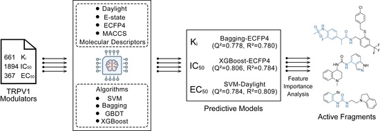
1. Introduction
2. Results and Discussion
2.1. Chemical Space and Scaffold Analysis
2.2. Feature Selection
2.3. Evaluation of Ki Activity Prediction Models
2.4. Evaluation of IC50 Activity Prediction Models
2.5. Evaluation of EC50 Activity Prediction Models
2.6. Y-Randomization Test
2.7. Model Interpretation
3. Materials and Methods
3.1. Data Collection and Processing
3.2. Descriptor Generation
3.3. Data Set Segmentation
3.4. Machine Learning Methods
3.5. Performance Evaluation Indicators
4. Conclusions
Author Contributions
Funding
Institutional Review Board Statement
Informed Consent Statement
Data Availability Statement
Conflicts of Interest
References
- Caterina, M.J.; Julius, D. The vanilloid receptor: A molecular gateway to the pain pathway. Annu. Rev. Neurosci. 2001, 24, 487–517. [Google Scholar] [CrossRef]
- Bevan, S.; Quallo, T.; Andersson, D.A. TRPV1. In Mammalian Transient Receptor Potential (TRP) Cation Channels: Volume I; Nilius, B., Flockerzi, V., Eds.; Springer: Berlin/Heidelberg, Germany, 2014; pp. 207–245. [Google Scholar]
- Iftinca, M.; Defaye, M.; Altier, C. TRPV1-Targeted Drugs in Development for Human Pain Conditions. Drugs 2021, 81, 7–27. [Google Scholar] [PubMed]
- Moran, M.M. TRP Channels as Potential Drug Targets. Annu. Rev. Pharmacol. Toxicol. 2018, 58, 309–330. [Google Scholar] [CrossRef] [PubMed]
- Domenichiello, A.F.; Ramsden, C.E. The silent epidemic of chronic pain in older adults. Prog. Neuropsychopharmacol. Biol. Psychiatry 2019, 93, 284–290. [Google Scholar] [PubMed]
- Gladkikh, I.N.; Sintsova, O.V.; Leychenko, E.V.; Kozlov, S.A. TRPV1 Ion Channel: Structural Features, Activity Modulators, and Therapeutic Potential. Biochemistry 2021, 86, S50–S70. [Google Scholar] [PubMed]
- Garami, A.; Shimansky, Y.P.; Rumbus, Z.; Vizin, R.C.L.; Farkas, N.; Hegyi, J.; Szakacs, Z.; Solymar, M.; Csenkey, A.; Chiche, D.A.; et al. Hyperthermia induced by transient receptor potential vanilloid-1 (TRPV1) antagonists in human clinical trials: Insights from mathematical modeling and meta-analysis. Pharmacol. Ther. 2020, 208, 107474. [Google Scholar] [PubMed]
- Moriello, A.S.; De Petrocellis, L.; Vitale, R.M. Fluorescence-Based Assay for TRPV1 Channels. In Endocannabinoid Signaling: Methods and Protocols; Maccarrone, M., Ed.; Springer: New York, NY, USA, 2023; pp. 119–131. [Google Scholar]
- Musella, A.; Centonze, D. Electrophysiology of Endocannabinoid Signaling. Methods Mol. Biol. 2023, 2576, 461–475. [Google Scholar]
- Li, Q.; Shah, S. Structure-Based Virtual Screening. Methods Mol. Biol. 2017, 1558, 111–124. [Google Scholar]
- Shaker, B.; Ahmad, S.; Lee, J.; Jung, C.; Na, D. In silico methods and tools for drug discovery. Comput. Biol. Med. 2021, 137, 104851. [Google Scholar]
- Kristam, R.; Parmar, V.; Viswanadhan, V.N. 3D-QSAR analysis of TRPV1 inhibitors reveals a pharmacophore applicable to diverse scaffolds and clinical candidates. J. Mol. Graph. Model. 2013, 45, 157–172. [Google Scholar]
- Kristam, R.; Rao, S.N.; D’Cruz, A.S.; Mahadevan, V.; Viswanadhan, V.N. TRPV1 antagonism by piperazinyl-aryl compounds: A Topomer-CoMFA study and its use in virtual screening for identification of novel antagonists. J. Mol. Graph. Model. 2017, 72, 112–128. [Google Scholar] [CrossRef] [PubMed]
- Wang, J.; Li, Y.; Yang, Y.; Du, J.; Zhang, S.; Yang, L. In silico research to assist the investigation of carboxamide derivatives as potent TRPV1 antagonists. Mol. Biosyst. 2015, 11, 2885–2899. [Google Scholar] [CrossRef] [PubMed]
- Melo-Filho, C.C.; Braga, R.C.; Andrade, C.H. 3D-QSAR approaches in drug design: Perspectives to generate reliable CoMFA models. Curr. Comput.-Aided Drug Des. 2014, 10, 148–159. [Google Scholar] [CrossRef] [PubMed]
- Yang, F.; Xiao, X.; Cheng, W.; Yang, W.; Yu, P.; Song, Z.; Yarov-Yarovoy, V.; Zheng, J. Structural mechanism underlying capsaicin binding and activation of the TRPV1 ion channel. Nat. Chem. Biol. 2015, 11, 518–524. [Google Scholar] [CrossRef]
- Rücker, C.; Rücker, G.; Meringer, M. y-Randomization and Its Variants in QSPR/QSAR. J. Chem. Inf. Model. 2007, 47, 2345–2357. [Google Scholar] [CrossRef]
- Szallasi, A.; Cortright, D.N.; Blum, C.A.; Eid, S.R. The vanilloid receptor TRPV1: 10 years from channel cloning to antagonist proof-of-concept. Nat. Rev. Drug Discov. 2007, 6, 357–372. [Google Scholar] [CrossRef]
- Aghazadeh Tabrizi, M.; Baraldi, P.G.; Baraldi, S.; Gessi, S.; Merighi, S.; Borea, P.A. Medicinal Chemistry, Pharmacology, and Clinical Implications of TRPV1 Receptor Antagonists. Med. Res. Rev. 2017, 37, 936–983. [Google Scholar] [CrossRef]
- Mendez, D.; Gaulton, A.; Bento, A.P.; Chambers, J.; De Veij, M.; Félix, E.; Magariños, M.P.; Mosquera, J.F.; Mutowo, P.; Nowotka, M.; et al. ChEMBL: Towards direct deposition of bioassay data. Nucleic Acids Res. 2019, 47, D930–D940. [Google Scholar] [CrossRef]
- Kim, S.; Chen, J.; Cheng, T.; Gindulyte, A.; He, J.; He, S.; Li, Q.; Shoemaker, B.A.; Thiessen, P.A.; Yu, B.; et al. PubChem in 2021: New data content and improved web interfaces. Nucleic Acids Res. 2021, 49, D1388–D1395. [Google Scholar] [CrossRef]
- Durant, J.L.; Leland, B.A.; Henry, D.R.; Nourse, J.G. Reoptimization of MDL Keys for Use in Drug Discovery. J. Chem. Inf. Comput. Sci. 2002, 42, 1273–1280. [Google Scholar] [CrossRef]
- Pearlman, R.S. Molecular Structure Description. The Electrotopological State by Lemont B. Kier (Virginia Commonwealth University) and Lowell H. Hall (Eastern Nazarene College). Academic Press: San Diego. 1999. xx + 245 pp. $99.95. ISBN 0-12-406555-4. J. Am. Chem. Soc. 2000, 122, 6340. [Google Scholar] [CrossRef]
- Rogers, D.; Hahn, M. Extended-Connectivity Fingerprints. J. Chem. Inf. Model. 2010, 50, 742–754. [Google Scholar] [CrossRef] [PubMed]
- Yang, Z.-Y.; Yang, Z.-J.; Lu, A.-P.; Hou, T.-J.; Cao, D.-S. Scopy: An integrated negative design python library for desirable HTS/VS database design. Brief. Bioinform. 2020, 22, bbaa194. [Google Scholar] [CrossRef] [PubMed]
- Landrum, G.; Sforna, G.; Winter, H.D. RDKit: Open-Source Cheminformatics, version 2020.09; 2006. Available online: https://www.rdkit.org/ (accessed on 15 August 2023).
- Pedregosa, F.; Varoquaux, G.; Gramfort, A.; Michel, V.; Thirion, B.; Grisel, O.; Blondel, M.; Prettenhofer, P.; Weiss, R.; Dubourg, V.; et al. Scikit-learn: Machine Learning in Python. J. Mach. Learn. Res. 2011, 12, 2825–2830. [Google Scholar]
- Cortes, C.; Vapnik, V. Support-vector networks. Mach. Learn. 1995, 20, 273–297. [Google Scholar] [CrossRef]
- Xu, J.; Wang, L.; Wang, L.; Shen, X.; Xu, W. QSPR study of Setschenow constants of organic compounds using MLR, ANN, and SVM analyses. J. Comput. Chem. 2011, 32, 3241–3252. [Google Scholar] [CrossRef]
- Friedman, J.H. Stochastic gradient boosting. Comput. Stat. Data Anal. 2002, 38, 367–378. [Google Scholar] [CrossRef]
- Chen, T.; Guestrin, C. XGBoost: A Scalable Tree Boosting System. In Proceedings of the 22nd ACM SIGKDD International Conference on Knowledge Discovery and Data Mining, San Francisco, CA, USA, 13–17 August 2016; Association for Computing Machinery: San Francisco, NY, USA, 2016; pp. 785–794. [Google Scholar]
- Breiman, L. Bagging predictors. Mach. Learn. 1996, 24, 123–140. [Google Scholar] [CrossRef]


| No. | Ki | IC50 | EC50 | |||
|---|---|---|---|---|---|---|
| Carbon Scaffold | Number | Carbon Scaffold | Number | Carbon Scaffold | Number | |
| 1 |  | 137 |  | 174 |  | 41 |
| 2 |  | 83 |  | 152 |  | 30 |
| 3 |  | 47 |  | 100 |  | 24 |
| 4 |  | 45 |  | 77 |  | 17 |
| 5 |  | 37 |  | 71 |  | 14 |
| 6 |  | 29 |  | 63 |  | 11 |
| 7 |  | 22 |  | 58 |  | 11 |
| 8 |  | 18 |  | 46 |  | 10 |
| 9 |  | 18 |  | 43 |  | 9 |
| 10 |  | 18 |  | 35 |  | 8 |
| Algorithm | Descriptor | ||||||
|---|---|---|---|---|---|---|---|
| SVM | Daylight | 0.725 ± 0.012 | 0.408 ± 0.009 | 0.317 ± 0.005 | 0.766 | 0.419 | 0.320 |
| E-state | 0.502 ± 0.010 | 0.550 ± 0.005 | 0.417 ± 0.006 | 0.536 | 0.590 | 0.448 | |
| ECFP4 | 0.744 ± 0.008 | 0.394 ± 0.006 | 0.318 ± 0.004 | 0.761 | 0.424 | 0.325 | |
| MACCS | 0.684 ± 0.006 | 0.438 ± 0.004 | 0.344 ± 0.004 | 0.687 | 0.485 | 0.362 | |
| Bagging | Daylight | 0.742 ± 0.018 | 0.395 ± 0.013 | 0.307 ± 0.009 | 0.779 | 0.408 | 0.312 |
| E-state | 0.677 ± 0.018 | 0.442 ± 0.012 | 0.348 ± 0.008 | 0.642 | 0.519 | 0.393 | |
| ECFP4 | 0.778 ± 0.012 | 0.367 ± 0.010 | 0.291 ± 0.008 | 0.780 | 0.407 | 0.305 | |
| MACCS | 0.697 ± 0.024 | 0.428 ± 0.016 | 0.334 ± 0.013 | 0.750 | 0.433 | 0.323 | |
| GBDT | Daylight | 0.723 ± 0.010 | 0.410 ± 0.007 | 0.326 ± 0.005 | 0.755 | 0.429 | 0.332 |
| E-state | 0.671 ± 0.013 | 0.447 ± 0.009 | 0.356 ± 0.007 | 0.623 | 0.532 | 0.410 | |
| ECFP4 | 0.759 ± 0.007 | 0.382 ± 0.005 | 0.309 ± 0.004 | 0.757 | 0.427 | 0.329 | |
| MACCS | 0.686 ± 0.011 | 0.437 ± 0.008 | 0.340 ± 0.007 | 0.703 | 0.472 | 0.371 | |
| XGBoost | Daylight | 0.723 ± 0.022 | 0.410 ± 0.015 | 0.317 ± 0.011 | 0.766 | 0.419 | 0.316 |
| E-state | 0.683 ± 0.032 | 0.438 ± 0.020 | 0.342 ± 0.014 | 0.648 | 0.514 | 0.385 | |
| ECFP4 | 0.771 ± 0.014 | 0.373 ± 0.011 | 0.301 ± 0.009 | 0.816 | 0.371 | 0.292 | |
| MACCS | 0.696 ± 0.020 | 0.429 ± 0.013 | 0.337 ± 0.011 | 0.745 | 0.437 | 0.330 |
| Algorithm | Descriptor | ||||||
|---|---|---|---|---|---|---|---|
| SVM | Daylight | 0.726 ± 0.006 | 0.424 ± 0.005 | 0.338 ± 0.004 | 0.744 | 0.443 | 0.353 |
| E-state | 0.487 ± 0.008 | 0.580 ± 0.004 | 0.455 ± 0.003 | 0.545 | 0.590 | 0.455 | |
| ECFP4 | 0.759 ± 0.006 | 0.398 ± 0.005 | 0.318 ± 0.004 | 0.763 | 0.426 | 0.342 | |
| MACCS | 0.639 ± 0.005 | 0.487 ± 0.004 | 0.381 ± 0.003 | 0.682 | 0.494 | 0.391 | |
| Bagging | Daylight | 0.719 ± 0.016 | 0.429 ± 0.012 | 0.343 ± 0.008 | 0.712 | 0.469 | 0.366 |
| E-state | 0.642 ± 0.020 | 0.485 ± 0.013 | 0.376 ± 0.010 | 0.628 | 0.534 | 0.426 | |
| ECFP4 | 0.757 ± 0.015 | 0.399 ± 0.012 | 0.318 ± 0.008 | 0.722 | 0.462 | 0.362 | |
| MACCS | 0.674 ± 0.017 | 0.462 ± 0.011 | 0.364 ± 0.008 | 0.681 | 0.494 | 0.396 | |
| GBDT | Daylight | 0.685 ± 0.007 | 0.455 ± 0.005 | 0.368 ± 0.003 | 0.706 | 0.475 | 0.378 |
| E-state | 0.555 ± 0.006 | 0.540 ± 0.003 | 0.428 ± 0.002 | 0.584 | 0.564 | 0.449 | |
| ECFP4 | 0.673 ± 0.004 | 0.463 ± 0.003 | 0.374 ± 0.003 | 0.703 | 0.477 | 0.386 | |
| MACCS | 0.579 ± 0.005 | 0.525 ± 0.003 | 0.418 ± 0.003 | 0.610 | 0.546 | 0.437 | |
| XGBoost | Daylight | 0.742 ± 0.020 | 0.411 ± 0.015 | 0.325 ± 0.011 | 0.746 | 0.441 | 0.347 |
| E-state | 0.660 ± 0.022 | 0.472 ± 0.014 | 0.368 ± 0.011 | 0.664 | 0.507 | 0.389 | |
| ECFP4 | 0.806 ± 0.013 | 0.357 ± 0.011 | 0.290 ± 0.007 | 0.784 | 0.407 | 0.328 | |
| MACCS | 0.699 ± 0.020 | 0.444 ± 0.014 | 0.349 ± 0.009 | 0.727 | 0.457 | 0.367 |
| Algorithm | Descriptor | ||||||
|---|---|---|---|---|---|---|---|
| SVM | Daylight | 0.784 ± 0.009 | 0.505 ± 0.010 | 0.409 ± 0.008 | 0.809 | 0.532 | 0.420 |
| E-state | 0.665 ± 0.013 | 0.629 ± 0.011 | 0.509 ± 0.012 | 0.716 | 0.649 | 0.492 | |
| ECFP4 | 0.772 ± 0.008 | 0.518 ± 0.009 | 0.416 ± 0.006 | 0.844 | 0.481 | 0.382 | |
| MACCS | 0.758 ± 0.010 | 0.534 ± 0.011 | 0.423 ± 0.011 | 0.751 | 0.607 | 0.488 | |
| Bagging | Daylight | 0.765 ± 0.015 | 0.527 ± 0.016 | 0.415 ± 0.013 | 0.718 | 0.647 | 0.492 |
| E-state | 0.725 ± 0.022 | 0.570 ± 0.022 | 0.454 ± 0.015 | 0.735 | 0.626 | 0.474 | |
| ECFP4 | 0.782 ± 0.017 | 0.507 ± 0.018 | 0.400 ± 0.016 | 0.844 | 0.480 | 0.367 | |
| MACCS | 0.746 ± 0.025 | 0.547 ± 0.025 | 0.431 ± 0.020 | 0.766 | 0.589 | 0.450 | |
| GBDT | Daylight | 0.772 ± 0.014 | 0.518 ± 0.015 | 0.408 ± 0.013 | 0.745 | 0.614 | 0.465 |
| E-state | 0.731 ± 0.019 | 0.563 ± 0.019 | 0.458 ± 0.012 | 0.777 | 0.575 | 0.428 | |
| ECFP4 | 0.775 ± 0.012 | 0.515 ± 0.013 | 0.402 ± 0.011 | 0.832 | 0.499 | 0.404 | |
| MACCS | 0.742 ± 0.012 | 0.552 ± 0.012 | 0.432 ± 0.012 | 0.759 | 0.597 | 0.475 | |
| XGBoost | Daylight | 0.771 ± 0.030 | 0.519 ± 0.030 | 0.409 ± 0.023 | 0.777 | 0.575 | 0.443 |
| E-state | 0.729 ± 0.026 | 0.566 ± 0.025 | 0.439 ± 0.022 | 0.772 | 0.581 | 0.445 | |
| ECFP4 | 0.778 ± 0.021 | 0.512 ± 0.022 | 0.395 ± 0.017 | 0.840 | 0.487 | 0.380 | |
| MACCS | 0.751 ± 0.019 | 0.542 ± 0.019 | 0.422 ± 0.016 | 0.699 | 0.668 | 0.501 |
Disclaimer/Publisher’s Note: The statements, opinions and data contained in all publications are solely those of the individual author(s) and contributor(s) and not of MDPI and/or the editor(s). MDPI and/or the editor(s) disclaim responsibility for any injury to people or property resulting from any ideas, methods, instructions or products referred to in the content. |
© 2024 by the authors. Licensee MDPI, Basel, Switzerland. This article is an open access article distributed under the terms and conditions of the Creative Commons Attribution (CC BY) license (https://creativecommons.org/licenses/by/4.0/).
Share and Cite
Wei, X.; Huang, T.; Yang, Z.; Pan, L.; Wang, L.; Ding, J. Quantitative Predictive Studies of Multiple Biological Activities of TRPV1 Modulators. Molecules 2024, 29, 295. https://doi.org/10.3390/molecules29020295
Wei X, Huang T, Yang Z, Pan L, Wang L, Ding J. Quantitative Predictive Studies of Multiple Biological Activities of TRPV1 Modulators. Molecules. 2024; 29(2):295. https://doi.org/10.3390/molecules29020295
Chicago/Turabian StyleWei, Xinmiao, Tengxin Huang, Zhijiang Yang, Li Pan, Liangliang Wang, and Junjie Ding. 2024. "Quantitative Predictive Studies of Multiple Biological Activities of TRPV1 Modulators" Molecules 29, no. 2: 295. https://doi.org/10.3390/molecules29020295