
Study of the Stability of Wine Samples for 1H-NMR Metabolomic Profile Analysis through Chemometrics Methods
 , , and
Abstract
:1. Introduction
2. Results and Discussion
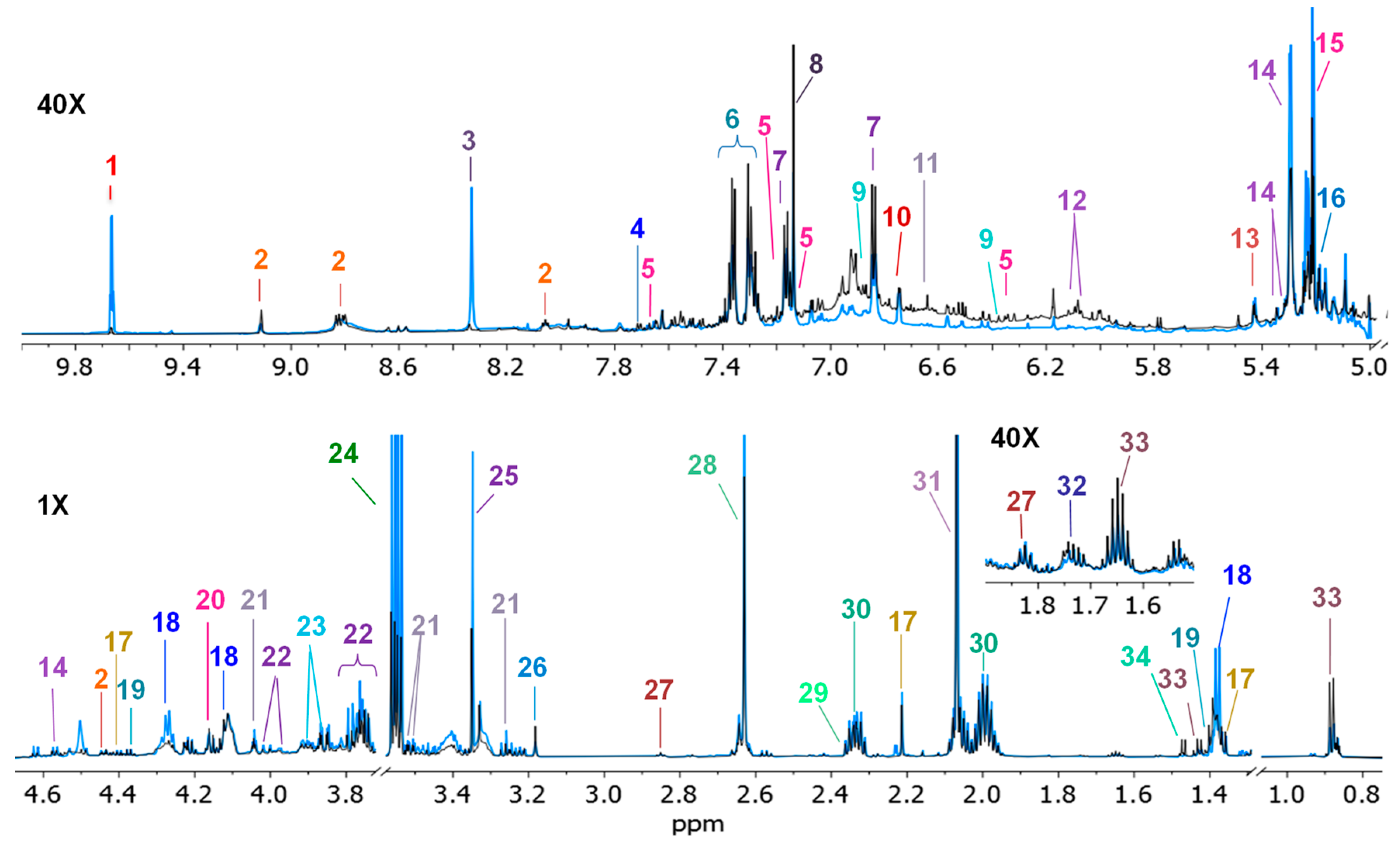
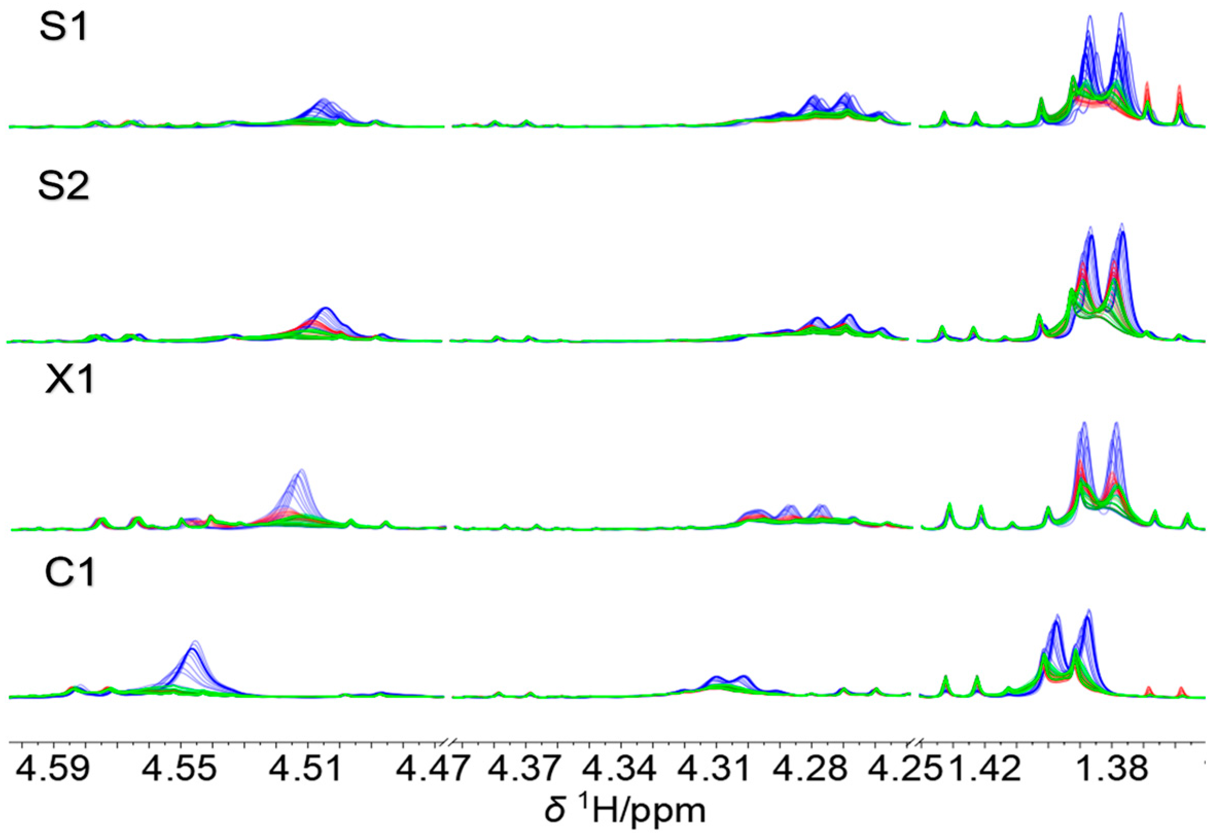
2.1. NMR Fingerprint
2.2. Chemometric Analyses
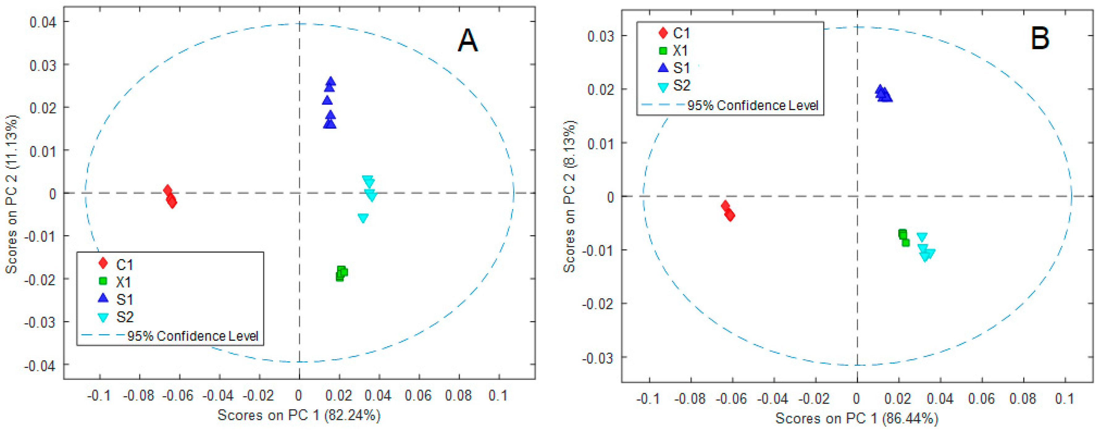
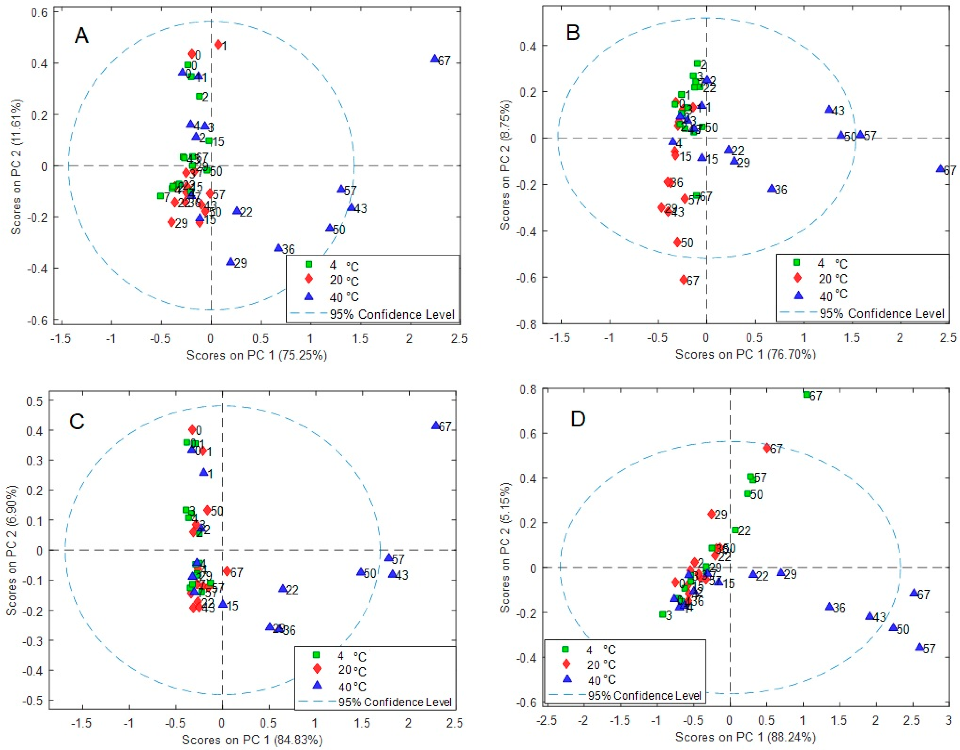
2.2.1. Principal Component Analysis (PCA)
2.2.2. ANOVA Simultaneous Component Analysis (ASCA)
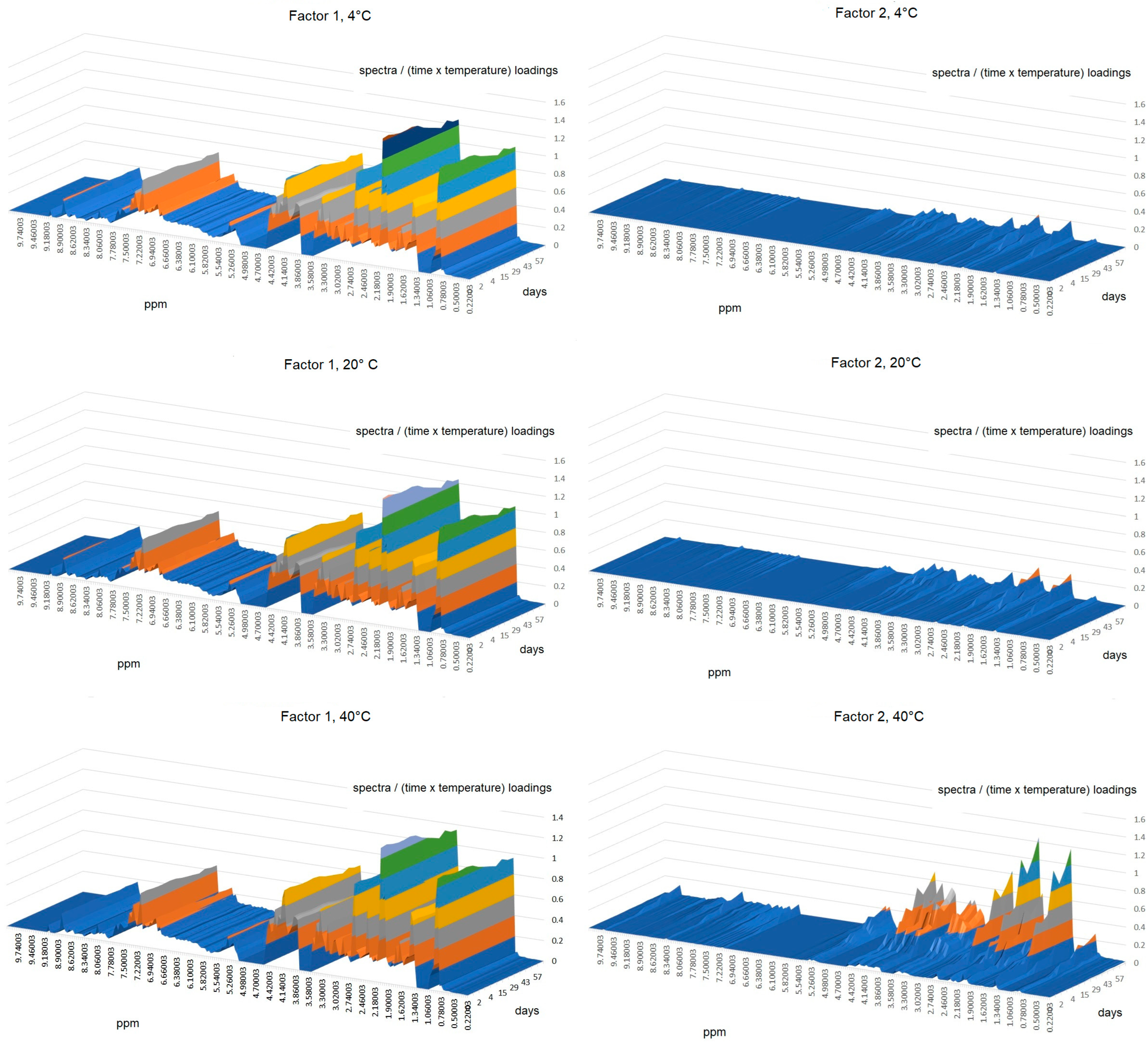
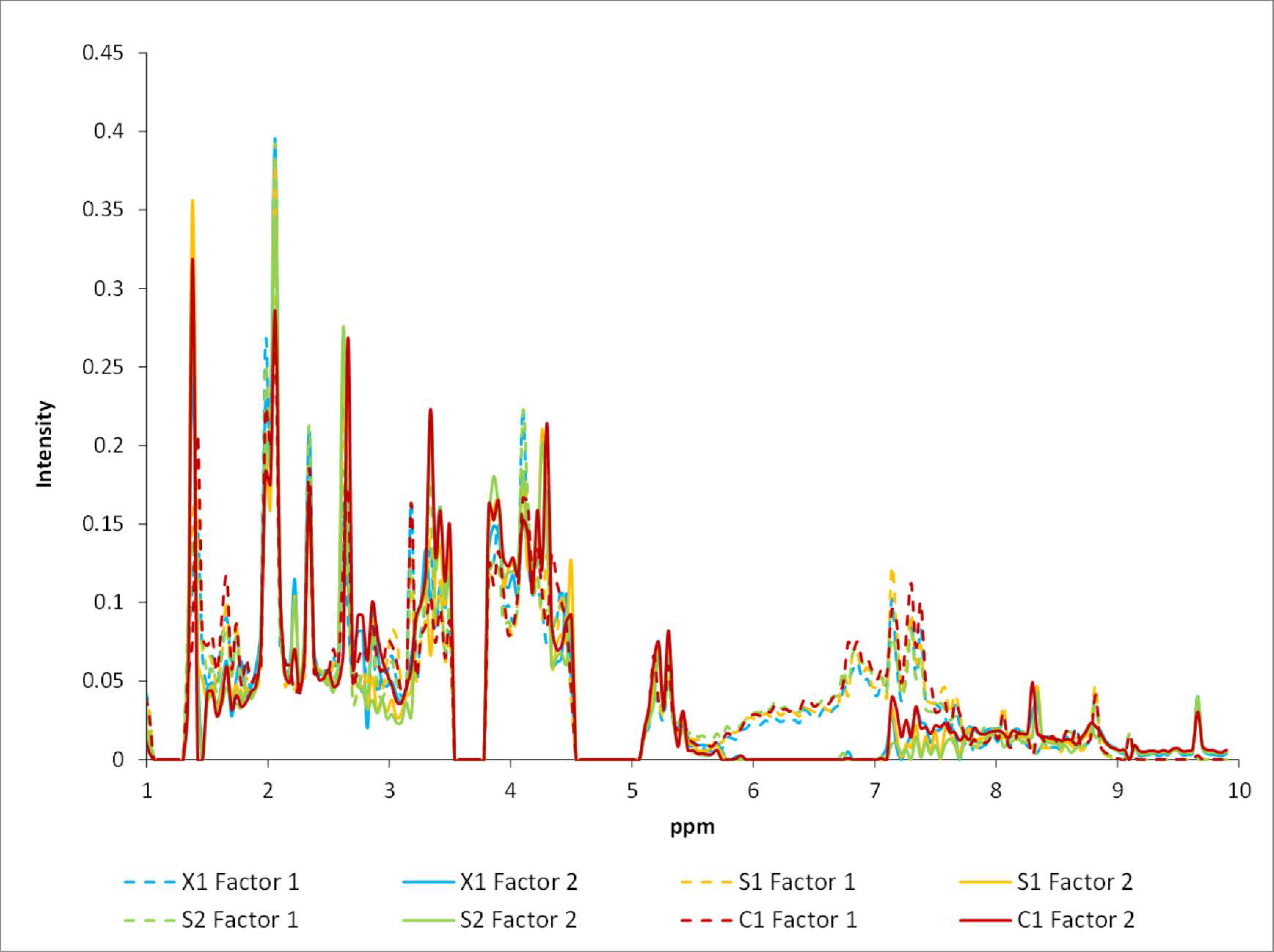
2.2.3. Parallel Factor Analysis (PARAFAC)
2.3. Metabolites Identification
3. Materials and Methods
3.1. Wine Samples
3.2. Sample Preparation and Storage Conditions
Control Samples
3.3. 1H-NMR Analysis
3.4. NMR Spectra Processing
3.5. Multivariate Data Analysis
3.6. Metabolite Profiling
4. Conclusions
Author Contributions
Funding
Institutional Review Board Statement
Informed Consent Statement
Data Availability Statement
Acknowledgments
Conflicts of Interest
Sample Availability
References
- Cozzolino, D. Metabolomics in grape and wine: Definition, current status and future prospects. Food Anal. Methods 2016, 9, 2986–2997. [Google Scholar] [CrossRef]
- Amargianitaki, M.; Spyros, A. NMR-based metabolomics in wine quality control and authentication. Chem. Biol. Technol. Agric. 2017, 4, 9. [Google Scholar] [CrossRef] [Green Version]
- Brescia, M.A.; Caldarola, V.; de Giglio, A.; Benedetti, D.; Fanizzi, F.P.; Sacco, A. Characterization of the geographical origin of Italian red wines based on traditional and nuclear magnetic resonance spectrometric determinations. Anal. Chim. Acta 2002, 458, 177–186. [Google Scholar] [CrossRef]
- Son, H.S.; Ki, M.K.; van den Berg, F.; Hwang, G.S.; Park, W.M.; Lee, C.H.; Hong, Y.S. 1H nuclear magnetic resonance-based metabolomic characterization of wines by grape varieties and production areas. J. Agric. Food Chem. 2008, 56, 8007–8016. [Google Scholar] [CrossRef] [PubMed]
- Hu, B.; Gao, J.; Xu, S.; Zhu, J.; Fan, X.; Zhou, X. Quality evaluation of different varieties of dry red wine based on nuclear magnetic resonance metabolomics. Appl. Biol. Chem. 2020, 63, 24. [Google Scholar] [CrossRef]
- Consonni, R.; Cagliani, L.R.; Guantieri, V.; Simonato, B. Identification of metabolic content of selected Amarone wine. Food Chem. 2011, 129, 693–699. [Google Scholar] [CrossRef]
- Nilsson, M.; Duarte, I.F.; Almeida, C.; Delgadillo, I.; Goodfellow, B.J.; Gil, A.M.; Morris, G.A. High-resolution NMR and diffusion-ordered spectroscopy of port wine. J. Agric. Food Chem. 2004, 52, 3736–3743. [Google Scholar] [CrossRef]
- Cassino, C.; Tsolakis, C.; Bonello, F.; Gianotti, V.; Osella, D. Wine evolution during bottle aging, studied by 1H NMR spectroscopy and multivariate statistical analysis. Food Res. Int. 2019, 116, 566–577. [Google Scholar] [CrossRef]
- Gougeon, L.; da Costa, G.; Le Mao, I.; Ma, W.; Teissedre, P.L.; Guyon, F.; Richard, T. Wine analysis and authenticity using 1H-NMR metabolomics data: Application to Chinese wines. Food Anal. Methods 2018, 11, 3425–3434. [Google Scholar] [CrossRef]
- Forino, M.; Picariello, L.; Lopatriello, A.; Moio, L.; Gambuti, A. New insights into the chemical bases of wine color evolution and stability: The key role of acetaldehyde. Eur. Food Res. Technol. 2020, 246, 733–743. [Google Scholar] [CrossRef]
- Rochfort, S.; Ezernieks, V.; Bastian, S.E.P.; Downey, M.O. Sensory attributes of wine influenced by variety and berry shading discriminated by NMR metabolomics. Food Chem. 2010, 121, 1296–1304. [Google Scholar] [CrossRef]
- Hong, Y.-S. NMR-based metabolomics in wine science. Magn. Reson. Chem. 2011, 49, S13–S21. [Google Scholar] [CrossRef] [PubMed]
- Aru, V.; Sørensen, K.M.; Khakimov, B.; Toldam-Andersen, T.B.; Engelsen, S.B. Cool—Climate red wines—Chemical composition and comparison of two protocols for 1H-NMR Analysis. Molecules 2018, 23, 160. [Google Scholar] [CrossRef] [Green Version]
- Bartel, J.; Krumsiek, J.; Theis, F.J. Statistical methods for the analysis of high-throughput metabolomics data. Comput. Struct. Biotechnol. J. 2013, 4, e201301009. [Google Scholar] [CrossRef] [Green Version]
- Papotti, G.; Bertelli, D.; Graziosi, R.; Silvestri, M.; Bertacchini, L.; Durante, C.; Plessi, M. Application of one- and two-dimensional NMR spectroscopy for the characterization of protected designation of origin Lambrusco wines of Modena. J. Agric. Food Chem. 2013, 61, 1741–1746. [Google Scholar] [CrossRef]
- Mascellani, A.; Hoca, G.; Babisz, M.; Krska, P.; Kloucek, P.; Havlik, J. 1H NMR chemometric models for classification of Czech wine type and variety. Food Chem. 2021, 339, 127852. [Google Scholar] [CrossRef] [PubMed]
- Hu, B.; Yue, Y.; Zhu, Y.; Wen, W.; Zhang, F.; Hardie, J.W. Proton Nuclear Magnetic Resonance-Spectroscopic discrimination of wines reflects genetic homology of several different grape (V. vinifera L.) cultivars. PLoS ONE 2015, 10, e0142840. [Google Scholar] [CrossRef]
- Fan, S.; Zhong, Q.; Fauhl-Hassek, C.; Pfister, M.K.H.; Horn, B.; Huang, Z. Classification of Chinese wine varieties using 1H NMR spectroscopy combined with multivariate statistical analysis. Food Control 2018, 88, 113–122. [Google Scholar] [CrossRef]
- Fu, Y.; Lim, L.T.; Kakuda, Y. Chemometric analysis of gas chromatographic data-investigation of enological parameters of a bag-in-box white wine as affected by storage time and temperature. J. Chemom. 2011, 25, 610–619. [Google Scholar] [CrossRef]
- Płotka-Wasylka, J.; Simeonov, V.; Namieśnik, J. Evaluation of the impact of storage conditions on the biogenic amines profile in opened wine bottles. Molecules 2018, 23, 1130. [Google Scholar] [CrossRef] [Green Version]
- Jung, R.; Kumar, K.; Patz, C.; Rauhut, D.; Tarasov, A.; Schüßler, C. Influence of transport temperature profiles on wine quality. Food Packag. Shelf Life 2021, 29, 100706. [Google Scholar] [CrossRef]
- Han, G.; Webb, M.R.; Waterhouse, A.L. Acetaldehyde reactions during wine bottle storage. Food Chem. 2019, 290, 208–215. [Google Scholar] [CrossRef] [PubMed]
- Bartowsky, E.J.; Henschke, P.A. Acetic acid bacteria spoilage of bottled red wine—A review. Int. J. Food Microbiol. 2008, 125, 60–70. [Google Scholar] [CrossRef] [PubMed]
- Makhotkina, O.; Kilmartin, P.A. Hydrolysis and formation of volatile esters in New Zealand Sauvignon blanc wine. Food Chem. 2012, 135, 486–493. [Google Scholar] [CrossRef]
- Ubeda, C.; Kania-Zelada, I.; del Barrio-Galán, R.; Medel-Marabolí, M.; Gil, M.; Peña-Neira, Á. Study of the changes in volatile compounds, aroma and sensory attributes during the production process of sparkling wine by traditional method. Food Res. Int. 2019, 119, 554–563. [Google Scholar] [CrossRef]
- Charnock, H.M.; Pickering, G.J.; Kemp, B.S. The Maillard reaction in traditional method sparkling wine. Front. Microbiol. 2022, 13, 979866. [Google Scholar] [CrossRef]
- Marques, L.; Espinosa, M.H.; Andrews, W.; Foster, R.T. Advancing flavor stability improvements in different beer types using novel electron paramagnetic resonance area and forced beer aging methods. J. Am. Soc. Brew. Chem. 2017, 75, 35–40. [Google Scholar] [CrossRef]
- The Metabolomics Innovation Centre FooDB. Available online: https://foodb.ca/ (accessed on 18 May 2023).


| Peak | Compound | δ 1H/ppm (Multiplicity, J in Hz, Assignation) |
|---|---|---|
| 1 | Acetaldehyde | 9.67 (q, 2.98, CH) |
| 2 | Trigonelline | 9.11 (s, COOH); 8.83 (d, 8.10, CH); 8.80 (d, 6.10, CH); 8.05 (t, CH); 4.42 (s, CH3) |
| 3 | Formic acid | 8.33 (s, CH3) |
| 4 | Cinnamic acid | 7.71 (d, 2 CH2) |
| 5 | Caffeic acid | 7.67 (d, 15.9, CH); 7.2 (d, 2.0, CH); 7.12 (dd, 8.3, 2.0); 6.46 (d, 15.8, CH) |
| 6 | Phenethyl alcohol | 7.37 (m, CH); 7.30 (m, CH); 3.75 (CH2OH); 2.77 (CH2) |
| 7 | Tyrosine | 7.17 (m, 2 CH); 6.84 (m, 2 CH) |
| 8 | Gallic acid | 7.14 (s, 2 CH) |
| 9 | p-Coumaric acid | 6.87 (d, 8.4, CH); 6,42 (d, 15.9, CH) |
| 10 | Shikimic acid | 6.75 (dd, 4.2, 2.2, CH) |
| 11 | Fumaric acid | 6.64 (s) |
| 12 | Epicatechin | 6.08 (d, 2.27, CH); 6.06 (d, 2.23, CH) |
| 13 | Sucrose | 5.43 (d, 3.6, CH); 4.57 (d, 7.7, CH) |
| 14 | Arabinose | 5.35 (d); 5.32 (d); 5.29 (d, 3.7, CH) |
| 15 | Trehalose | 5.22 (d, 3.6) |
| 16 | Glucose | 5.19 (d, 3.6, CH); 4.55 (d, 6.55, CH) |
| 17 | Acetoin | 4.40 (q, 7.1, CH); 2.2 (s, CH3); 1.36 (d, 7.2, CH3OH) |
| 18 | Ethyl lactate | 4.27 (q, 7.0 CH2); 4.11 (m, CH2); 1.38 (d, 6.9, CH3); 1.26 (t, CH3) |
| 19 | Lactic acid | 4.38 (q, 7.0); 1.40 (d, 6.9) |
| 20 | Ethyl acetate | 4.16 (q, 7.1, CH2); 1.24 (t, CH3) |
| 21 | Myo-inositol | 4.04 (t, 3.02, CH); 3.52 (dd, 9.98, 2.85, CH); 3.26 (t, 9.37, CH) |
| 22 | Fructose | 4.01 (m); 3.98 (m); 3.77 (m) |
| 23 | Mannitol | 3.86 (dd, 2.9 and 11.8, CH2); 3.79 (d, 8.71, CH2) |
| 24 | Glycerol * | 3.77 (m, CH); 3.55 (dd, 11.4 and 6.4, CH2) |
| 25 | Methanol | 3.35(s, CH3) |
| 26 | Choline | 3.18 (s, 3 CH3) |
| 27 | GABA | 2.85 (t, 6.8, CH2); 2.42 (t, 7.5, CH2); 1.83 (p, 7.7, CH2) |
| 28 | Succinic acid | 2.63(s, 2 CH2) |
| 29 | Pyuvic acid | 2.3(s, CH3) |
| 30 | Proline | 2.3(m, CH2); 2.0(m, CH2) |
| 31 | Acetic acid | 2.07(s, CH3) |
| 32 | 1,3-propanediol | 1.73 (q, 6.7 Hz, 1H) |
| 33 | Isopentanol | 1.65 (hept, 6.7, CH); 1.43 (q, 6.94, CH2; 0.88 (d, 6.75, 2 CH3) |
| 34 | Alanine | 1.47 (d, 6.5, CH3) |
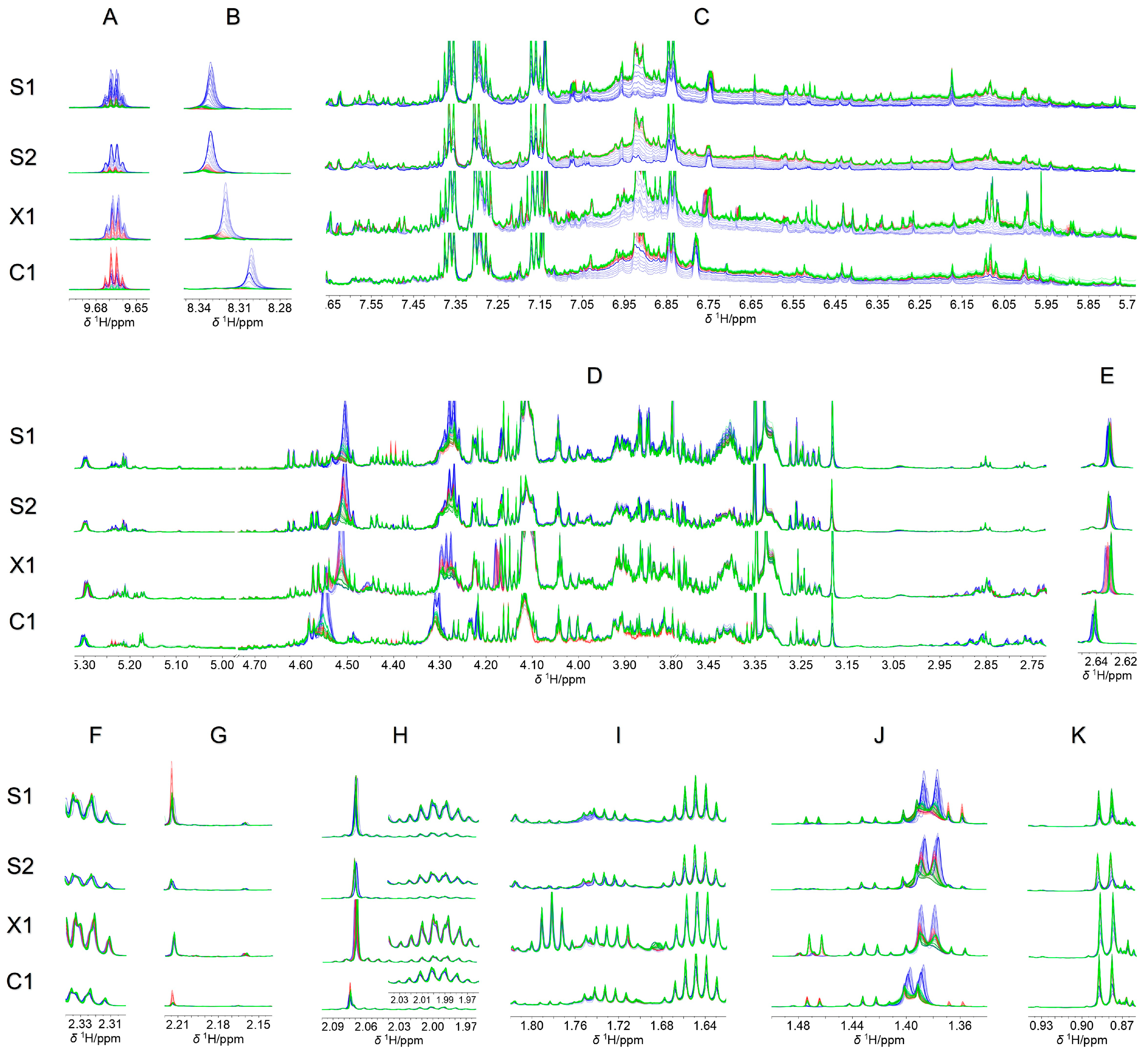
| Figure 12 | Bucket (ppm) | Assigned Metabolite |
|---|---|---|
| A | 9.70–9.62 | Acetaldehyde |
| B | 8.34–8.26 | Formic acid |
| C | 7.70–5.82 | Polyphenols |
| D | 5.30–5.18 4.58–4.46 4.38–4.18 4.14–4.10 4.02–3.78 3.50–2.74 | Carbohydrates, Lactic acid, Ethyl lactate, Methanol, Choline, and others |
| E | 2.66–2.62 | Succinic acid |
| F | 2.34–2.30 | Proline |
| G H | 2.22–2.14 2.10–1.98 | Acetoin, Proline, Acetic acid, and others |
| I | 1.82–1.62 | 1,3-propanediol, Isopentanol, and others |
| J | 1.50–1.34 | Alanine, Isopentanol, Lactic acid, and Acetoin |
| K | 0.94–0.86 | Higher alcohols and amino acids |
Disclaimer/Publisher’s Note: The statements, opinions and data contained in all publications are solely those of the individual author(s) and contributor(s) and not of MDPI and/or the editor(s). MDPI and/or the editor(s) disclaim responsibility for any injury to people or property resulting from any ideas, methods, instructions or products referred to in the content. |
© 2023 by the authors. Licensee MDPI, Basel, Switzerland. This article is an open access article distributed under the terms and conditions of the Creative Commons Attribution (CC BY) license (https://creativecommons.org/licenses/by/4.0/).
Share and Cite
García-Aguilera, M.E.; Delgado-Altamirano, R.; Villalón, N.; Ruiz-Terán, F.; García-Garnica, M.M.; Ocaña-Ríos, I.; Rodríguez de San Miguel, E.; Esturau-Escofet, N. Study of the Stability of Wine Samples for 1H-NMR Metabolomic Profile Analysis through Chemometrics Methods. Molecules 2023, 28, 5962. https://doi.org/10.3390/molecules28165962
García-Aguilera ME, Delgado-Altamirano R, Villalón N, Ruiz-Terán F, García-Garnica MM, Ocaña-Ríos I, Rodríguez de San Miguel E, Esturau-Escofet N. Study of the Stability of Wine Samples for 1H-NMR Metabolomic Profile Analysis through Chemometrics Methods. Molecules. 2023; 28(16):5962. https://doi.org/10.3390/molecules28165962
Chicago/Turabian StyleGarcía-Aguilera, Martha E., Ronna Delgado-Altamirano, Nayelli Villalón, Francisco Ruiz-Terán, Mariana M. García-Garnica, Irán Ocaña-Ríos, Eduardo Rodríguez de San Miguel, and Nuria Esturau-Escofet. 2023. "Study of the Stability of Wine Samples for 1H-NMR Metabolomic Profile Analysis through Chemometrics Methods" Molecules 28, no. 16: 5962. https://doi.org/10.3390/molecules28165962