A Valence-Bond-Based Multiconfigurational Density Functional Theory: The λ-DFVB Method Revisited

Abstract

A recently developed valence-bond-based multireference density functional theory, named λ-DFVB, is revisited in this paper. λ-DFVB remedies the double-counting error of electron correlation by decomposing the electron–electron interactions into the wave function term and density functional term with a variable parameter λ. The λ value is defined as a function of the free valence index in our previous scheme, denoted as λ-DFVB(K) in this paper. Here we revisit the λ-DFVB method and present a new scheme based on natural orbital occupation numbers (NOONs) for parameter λ, named λ-DFVB(IS), to simplify the process of λ-DFVB calculation. In λ-DFVB(IS), the parameter λ is defined as a function of NOONs, which are straightforwardly determined from the many-electron wave function of the molecule. Furthermore, λ-DFVB(IS) does not involve further self-consistent field calculation after performing the valence bond self-consistent field (VBSCF) calculation, and thus, the computational effort in λ-DFVB(IS) is approximately the same as the VBSCF method, greatly reduced from λ-DFVB(K). The performance of λ-DFVB(IS) was investigated on a broader range of molecular properties, including equilibrium bond lengths and dissociation energies, atomization energies, atomic excitation energies, and chemical reaction barriers. The computational results show that λ-DFVB(IS) is more robust without losing accuracy and comparable in accuracy to high-level multireference wave function methods, such as CASPT2.

1. Introduction

The electronic structure calculations of strongly correlated systems, which cannot be well described by a single configuration space function, are still challenging in the methodology development of electronic structure theory. Typical strongly correlated problems occur in the excited states; transition states; open-shell molecules, especially the radical species and systems that contain transition-metal atoms; and the bond dissociation process, etc. Obtaining a proper description of such systems usually requires a method capable of describing both static and dynamic electron correlations.

The complete active space self-consistent field (CASSCF) [1] is a widely used quantum chemistry method able to capture static correlation. In valence bond (VB) theory, the valence bond self-consistent field (VBSCF) [2,3], which is a multiconfigurational self-consistent field (MCSCF) analog with atomic orbitals (AOs), covers the static correlation by expressing the many-electron wave function of the molecule as a linear combination of VB structures. To cover dynamic correlations within the CASSCF scheme, post-CASSCF methods are required, such as the complete active space second-order perturbation theory (CASPT2) [4] and multireference configuration interaction (MRCI) [5]. Their analogs are present in VB theory, valence bond configuration interaction (VBCI) [6,7], and valence bond perturbation theory (VBPT2) [8,9], respectively. However, the computational costs of both methods are still expensive, compared to their MO analogs.

Kohn−Sham density functional theory (KS-DFT) [10,11] has played a very important role in electronic structure calculation in chemistry, biochemistry, and solid state due to its affordable computational cost with satisfactory accuracy. Due to the fact that the exact formula of the exchange–correlation functional is still unknown, KS-DFT currently suffers from a difficulty in tackling molecular systems with a strong multireference character, which cannot be described well by using a single Slater determinant. One of the straightforward schemes is to combine CASSCF with DFT, namely multireference density functional theory (MRDFT), where CASSCF takes care of the static correlation, while DFT describes the dynamic correlation. Various MRDFT schemes have been proposed to properly describe strongly correlated systems [12,13,14,15,16,17,18,19,20,21,22,23,24,25,26,27,28,29]. One of the problems that should be solved in MRDFT is the double-counting error (DCE), which is due to the fact that static and dynamic correlations cannot be separated strictly. By using on-top pair density, various DCE-free MRDFT methods have been proposed over the last two decades [25,30,31,32,33,34]. Among them, one of the representative MRDFT methods is multiconfiguration pair-density functional theory (MC-PDFT), which avoids the DCE by calculating the kinetic and Coulomb contributions of the wave function part, and the rest of the part is obtained from a pair-density functional [25].

In a similar fashion, the strategy of hybrid VB theory with DFT has been implemented, such as VBDFT(s) [35,36,37,38], VB-DFT [39], and DFVB [40,41,42]. Recently, a newly developed MRDFT scheme based on the valence bond wave function, namely the λ-density functional valence bond (λ-DFVB) method [42], was presented. This method is inspired by the MC1H approximation proposed by Sharkas et al. [22]. The MC1H approach combines the MCSCF with DFT by linear decomposition of the electron−electron interaction with a single parameter λ, which is set to a fixed value of 0.25. Different from Sharkas’s scheme, the λ value in λ-DFVB is variable and ranges from 0 to 1, depending on the multireference character of the studied molecule. The stronger the multireference character, the larger value taken in the calculation. To describe the extent of the multireference character, the molecular free valence index K is used in λ-DFVB, and the functional form of λ is taken tentatively as λ = K^1/4. The molecular free valence index K is defined by the total atomic free valences and the bond orders of the molecule, expressed in terms of the overlap and spin density matrices [42].

Estimates of the multireference character have been explored by various approaches. Among them, indices based on the natural orbital occupation numbers (NOONs) are widely used, which are given by diagonalizing the density matrix of the molecule. Various schemes have been proposed, such as von Neumann entropy S [43], correlation entropy S₂ [44], the M diagnostic [45], and the I_ND diagnostic [46]. The purpose of this paper is to revisit the λ-DFVB method by employing the NOONs to determine the value of parameter λ to simplify the procedure of λ-DFVB calculation. Different from the molecular free valence index, which is defined by the total density matrix and spin density matrix as well as orbital overlaps, NOONs are straightforwardly obtained from the density matrix of the studied molecule. Moreover, the concept of bond order used in λ-DFVB(K) is somehow ambiguous if one performs λ-DFVB calculation for atomic systems.

In this paper, we revisit the λ-DFVB method and present a new scheme based on NOONs for parameter λ, named λ-DFVB(IS), instead of the molecular free valence index K used in the previous λ-DFVB scheme, which is denoted as λ-DFVB(K). Furthermore, to improve the practicality of the λ-DFVB method, some technical considerations are investigated in this paper to further simplify the process of λ-DFVB calculation.

2. Methodology

In VB theory, a many-electron wave function is expanded as a linear combination of Heitler−London−Slater−Pauling (HLSP) functions [47,48],

$$\mathsf{\Psi }={\displaystyle \sum _K{C}_K{\mathsf{\Phi }}_K}$$

(1)

where Φ_K is a specific VB structure, and C_K is the corresponding coefficient. The HLSP function Φ_K can be expressed as follows

$${\mathsf{\Phi }}_K=\widehat{A}{\mathsf{\Omega }}_0{\mathsf{\Theta }}_K$$

(2)

where $\widehat{A}$ is the antisymmetrizing operator, and Ω₀ is a direct product of orbitals {ϕ_i} as

$${\mathsf{\Omega }}_0={\varphi }_1\left(1\right){\varphi }_2\left(2\right)\cdots {\varphi }_N\left(N\right)$$

(3)

and Θ_K is a spin-paired spin eigenfunction [49], defined as

$${\mathsf{\Theta }}_K={\displaystyle \prod _{\left(ij\right)}{2}^{-1/2}\left[\alpha \left(i\right)\beta \left(i\right)-\beta \left(i\right)\alpha \left(j\right)\right]}{\displaystyle \prod _k\alpha \left(k\right)}$$

(4)

where (ij) runs over all bonds and k over all unpaired electrons.

The total energy and structure coefficients can be obtained by solving the standard secular equation

$$HC=EMC$$

(5)

where H, M, and C are the VB Hamiltonian, overlap, and coefficient matrices, respectively. The weight of a given VB structure, W_K, can be evaluated by the Coulson–Chirgwin formula [50],

$$W_K={\displaystyle \sum _L{C}_K{C}_L{M}_{KL}}$$

(6)

As the wave function theory (WFT) of electronic structure, there are various levels in ab initio classical VB methods, such as the valence bond self-consistent field (VBSCF) [2,3], breathing orbital valence bond (BOVB) [51,52,53], valence bond configuration interaction (VBCI) [6,7], and valence bond second-order perturbation theory (VBPT2) [8,9]. The VBSCF method is the elementary method of ab initio classical VB theory, where both VB structure coefficients {C_K} and VB orbitals {ϕ_i} are optimized simultaneously to minimize the total energy.

The λ-DFVB method incorporates the dynamic energy into VB theory using KS-DFT by expressing the total electronic energy of a molecule as

$$E^{\mathsf{\lambda }-DFVB}=\underset{\mathsf{\Psi }}{min}\left\{〈\mathsf{\Psi }|T+V_{ext}+\mathsf{\lambda }{W}_{\mathrm{e}\mathrm{e}}\left|\mathsf{\Psi }\right.〉+E_{HXC}^{\mathsf{\lambda }-DFVB}[\rho ]\right\}$$

(7)

where T, V_ext, and W_ee are the kinetic energy, external potential, and electron–electron interaction operators, respectively; $E_{HXC}^{\mathsf{\lambda }-DFVB}[\rho ]$ is the complement λ-dependent Hartree–exchange–correlation density functional for electronic density ρ; and λ is a coupling parameter. The first term in Equation (7) is computed by a normal VB route, while the second term, $E_{HXC}^{\mathsf{\lambda }-DFVB}[\rho ]$, is calculated by the KS-DFT method and includes four components

$$E_{HXC}^{\mathsf{\lambda }-DFVB}[\rho ]=(1-\mathsf{\lambda })\left(E_{\mathrm{H}}[\rho ]+E_{\mathrm{X}}[\rho ]\right)+\left(1-{\mathsf{\lambda }}^2\right)E_{\mathrm{C}}[\rho ]+{\mathsf{\lambda }}^2{E}_{\mathrm{C}}[{\rho }^{LD}]$$

(8)

where $E_{\mathrm{H}}[\rho ]$ is the Hartree energy, $E_{\mathrm{X}}[\rho ]$ is the exchange functional, and $E_{\mathrm{C}}[\rho ]$ is the correlation functional. Different from the multiconfigurational one-parameter hybrid (MC1H) approach [22], an extra term of the correlation energy, $E_{\mathrm{C}}[{\rho }^{LD}]$, is included, which is the correlation functional for the determinant that shares the largest coefficient in the VBSCF wave function.

As discussed in the previous paper, the parameter λ in Equation (7) scales the hybrid extent of the WFT and the KS-DFT method. Based on the fact that the VBSCF method covers the static correlation, it is thus suitable for molecules with a multireference character, while KS-DFT is a good tool for capturing the dynamic correlation. As such, it is more reasonable to allow the value of λ to be different for molecules with different extents of static and dynamic correlations.

In λ-DFVB(K), parameter λ is defined as a function of the molecular free valence index K,

$$\mathsf{\lambda }=K^{1/4}$$

(9)

The molecular free valence index K is defined as

$$K=\frac{{\displaystyle \sum _{\mathrm{A}}{F}_{\mathrm{A}}}}{{\displaystyle \sum _{\mathrm{A}}{V}_{\mathrm{A}}}}$$

(10)

$$F_{\mathrm{A}}=V_{\mathrm{A}}-{\displaystyle \sum _{B,B\ne A}{O}_{AB}}$$

(11)

$$V_{\mathrm{A}}={\displaystyle \sum _{\mu \in \mathrm{A}}2{\left(DS\right)}_{\mu \mu }}-{\displaystyle \sum _{\mu ,\nu \in \mathrm{A}}{\left(DS\right)}_{\mu \nu }{\left(DS\right)}_{\nu \mu }}$$

(12)

$$O_{AB}={\displaystyle \sum _{\mu \in \mathrm{A}}{\displaystyle \sum _{\nu \in \mathrm{B}}\left[{\left(DS\right)}_{\mu \nu }{\left(DS\right)}_{\nu \mu }+{\left({\mathbf{P}}^s\mathbf{S}\right)}_{\mu \nu }{\left({\mathbf{P}}^s\mathbf{S}\right)}_{\nu \mu }\right]}}$$

(13)

where F_A and V_A are the free valence and total valence of atom A [54], O_AB is the bond order between atoms A and B, S is the overlap matrix between the basis functions, and D and P^s are the total and spin polarization density matrices, respectively. The value of K ranges from 0 to 1, as F_A is identical to V_A in the dissociation limit.

Equation (7) can be implemented by a modified VBSCF route [42]. To this end, the structure coefficients {C_K} and orbitals {ϕ_i} are optimized by minimizing

$${\epsilon }_{}^{\mathsf{\lambda }-DFVB}=\left.〈\mathsf{\Psi }\right|T+V_{ext}+\mathsf{\lambda }{W}_{ee}+{\displaystyle \int d\mathit{r}{v}_{HXC}^{\mathsf{\lambda }-DFVB}\left[\rho \right]n\left(\mathit{r}\right)}\left|\mathsf{\Psi }\right.〉$$

(14)

where $n\left(\mathit{r}\right)$ is the density operator, and potential $v_{HXC}^{\mathsf{\lambda }-DFVB}\left[\rho \right]$ is defined as

$$v_{HXC}^{\mathsf{\lambda }-DFVB}\left[\rho \right]=\frac{\delta E_{HXC}^{\mathsf{\lambda }-DFVB}\left[\rho \right]}{\delta \rho }$$

(15)

In implementation, the potential $v_{HXC}^{\mathsf{\lambda }-DFVB}\left[\rho \right]$ is expressed in terms of one-electron integrals and λ-scaled two-electron integrals of the basis functions. The total electronic energy of the molecule is computed with the optimized {C_K} and {ϕ_i}, which is expressed as

$$E_{}^{\mathsf{\lambda }-DFVB}={\epsilon }_{}^{\mathsf{\lambda }-DFVB}+E_{HXC}^{\mathsf{\lambda }-DFVB}\left[\rho \right]-\left.〈\mathsf{\Psi }\right|{\displaystyle \mathsf{\int }d\mathit{r}{v}_{HXC}^{\mathsf{\lambda }-DFVB}\left[\rho \right]n\left(\mathit{r}\right)}\left|\mathsf{\Psi }\right.〉$$

(16)

Before performing a modified VBSCF calculation, a normal VBSCF is done for determining the value of parameter λ. Thus, the λ-DFVB(K) calculation is composed of the following steps:

(1)

Perform a normal VBSCF calculation to obtain the VBSCF density matrix;

(2)

Determine the λ value with Equations (9)–(13);

(3)

Compute the complement Hartree–exchange–correlation functional, $E_{HXC}^{\mathsf{\lambda }-DFVB}[\rho ]$ with Equation (8);

(4)

Build potential $v_{HXC}^{\mathsf{\lambda }-DFVB}\left[\rho \right]$ in terms of one-electron integrals with Equation (15);

(5)

Optimize {C_K} and {ϕ_i} by a modified VBSCF route, Equation (14);

(6)

Compute the λ-DFVB energy by Equation (16) with the optimized {C_K} and {ϕ_i}.

As can be seen above, the most time consuming occurs in Steps (1) and (5), which involve SCF iterations. Thus, the computational effort for λ-DFVB(K) is approximately two times that of VBSCF.

To determine the value of parameter λ in λ-DFVB(K), one should compute the free valence F_A and total valence V_A, as well as the bond order O_AB, for all atoms, which are defined with the density and overlap matrices of the basis functions. It can be shown that for closed-shell molecules, the summation of free valence F_A over all atoms actually equals the number of effectively unpaired electrons (EUEs), N_D,

$${\displaystyle \sum _{\mathrm{A}}{F}_{\mathrm{A}}}=N_{\mathrm{D}}={\displaystyle \sum _i{n}_i\left(2-n_i\right)}$$

(17)

where n_i is the natural orbital occupation numbers. It is worth noting that the number of EUEs and their variants have been widely used for estimating the static correlation character of a molecule [46,55,56,57,58,59]. To simplify the definition of parameter λ, the number of EUEs is used in this paper, instead of K. To ensure that the value of the index lies between 0 and 1, a normalized index based on EUEs is defined as

$$I_s=\frac{N_{\mathrm{D}}}{2n-n^2/m}$$

(18)

where n and m are the numbers of active electrons and active orbitals, respectively. The details of deduction for Equation (17) and the normalization factor in Equation (18) are presented in Appendix A.

In a similar fashion to λ-DFVB(K), parameter λ is defined by a function of I_s, as

$$\mathsf{\lambda }=I_s{}^{1/4}$$

(19)

Obviously, the range of the λ value is from 0 to 1, the same as I_s. Thus, the new scheme of λ-DFVB is denoted as λ-DFVB(IS). Now index I_s depends only on the NOONs, which are given by diagonalizing the density matrix of the molecule. Clearly, λ-DFVB(IS) gets rid of a set of intermediate quantities, such as free valence, total valence, and bond order, making the scheme more concise.

Furthermore, the numerical investigation shows that the optimized orbitals given from Step (1) in λ-DFVB(K) are virtually the same as the orbitals optimized in Step (5). As such, in λ-DFVB(IS), Step (5) is skipped, and only one SCF iteration process, Step (1), is required. That is to say, λ-DFVB(IS) is a post-VBSCF method, where VB orbitals and the density matrix are given at the VBSCF level, and the Hartree–exchange–correlation density functional is computed with the VBSCF density. Thus, the λ-DFVB(IS) energy is expressed as

$$E_{}^{\mathsf{\lambda }-DFVB}=E^{VBSCF}\left(\mathsf{\lambda }\right)+E_{HXC}^{\mathsf{\lambda }-DFVB}\left[\rho \right]$$

(20)

where E^VBSCF(λ) is VBSCF energy with the λ-dependent scaled two-electron integrals.

The implementation of λ-DFVB(IS) includes the following four steps:

(1)

Perform a normal VBSCF calculation to obtain the VBSCF density matrix;

(2)

Compute NOONs {n_i} from the VBSCF wave function, and get the λ value using Equation (19);

(3)

Compute the complement Hartree–exchange–correlation functional, $E_{HXC}^{\mathsf{\lambda }-DFVB}[\rho ]$ with Equation (8);

(4)

Compute the λ-DFVB(IS) energy by Equation (20).

It is obvious that the current scheme, λ-DFVB (IS), is much simpler than the old scheme, λ-DFVB(K).

3. Computational Details

All the VB calculations were implemented in the Xiamen Valence Bond (XMVB) package [60,61] using full VB structures and overlap-enhanced orbitals (OEOs), while the KS-DFT calculation were performed by the Gaussian 16 program [62]. The BLYP [63,64] functional was used for all λ-DFVB calculations. For comparison, CASPT2 calculations were also performed using OpenMolcas [65], with a standard imaginary shift of 0.2 Hartrees and the default IPEA shift of 0.25 Hartrees.

Test calculations can be classified into four sets: potential energy curves, atomization energies, excitation energies, and reaction barrier heights. For the potential energy curves, some diatomic molecules were investigated, including H₂, N₂, C₂, F₂, and HF. To assess the performance of atomization energies, the AE6 dataset [66] was used, which consists of SiH₄, S₂, SiO, C₃H₄, C₂H₂O₂, and C₄H₈. The excitation energies of several main group atoms, Be, C, N, N⁺, O, and O⁺, were also investigated. Finally, a series of reaction barriers in the DBH24 dataset [67] were studied, which contains 12 reactions with both forward and reverse reaction barrier heights.

The basis set used for the potential energy curves, atomization energies, and excitation energies was the cc-pVTZ basis set [68], while for the reaction barriers, the maug-cc-pVTZ basis set [69] was used. The geometries for the molecules in the AE6 and DBH24 datasets were taken from the Minnesota Database 2019 [70].

4. Results and Discussion

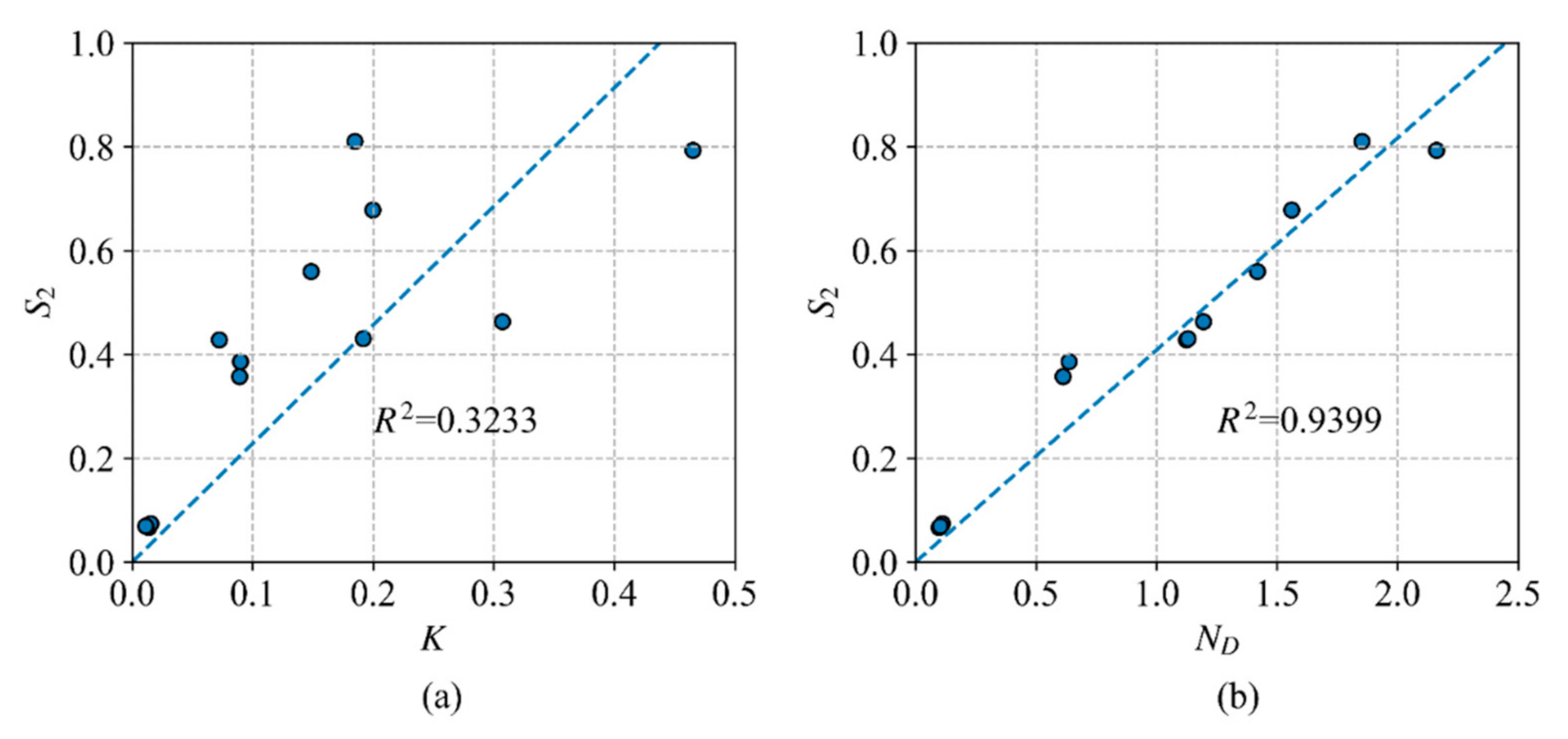
4.1. The Validity of the N_D Index

In order to validate the use of N_D in measuring the static correlation, Figure 1 shows the plots of the correlation entropy $S_2=-{\displaystyle \sum _i\left(n_i/2\right)\mathrm{l}\mathrm{n}\left(n_i/2\right)}$, which is widely used for diagnosing the extent of the multireference character versus the free valence index K (a) and the number of effectively unpaired electrons, the N_D index, (b) for the transition states in the DBH24 datasets computed by VBSCF. As can be seen from Figure 1, index N_D shares a stronger correlation with S₂ than index K. The value of R² for S₂ vs. N_D is 0.9399, and it is 0.3233 for S₂ vs. K. Figure 1 shows that it may be more reliable to use index N_D for the λ-DFVB method, instead of index K.

4.2. Dissociation of Diatomic Molecules

The results of the equilibrium bond lengths and bond dissociation energies calculated by various methods are presented in

Table 1. Deviation values of the equilibrium bond lengths (R_e, in Å) of diatomic molecules.

	Active Space	CASPT2	VBSCF	λ-DFVB		BLYP	B3LYP	Ref. 1
				K	IS
H2	(2, 2)	0.004	0.014	0.003	0.003	0.005	0.002	0.741
F2	(2, 2)	0.007	0.055	−0.040	−0.035	0.020	−0.015	1.412
HF	(2, 2)	−0.001	−0.001	−0.009	−0.008	0.016	0.005	0.917
N2	(6, 6)	0.005	0.005	0.000	−0.003	0.005	−0.007	1.098
C2	(8, 8)	0.007	0.012	0.008	0.008	0.013	0.004	1.243
	MUE	0.005	0.017	0.012	0.011	0.012	0.007

¹ The reference values are taken from [71].

and

Table 2. Deviation values of the bond dissociation energies (D_e, in kcal/mol) of diatomic molecules.

	Active Space	CASPT2	VBSCF	λ-DFVB		BLYP	B3LYP	Ref. 1
				K	IS
H2	(2, 2)	−3.6	−14.2	−1.0	−1.1	0.0	0.7	109.5
F2	(2, 2)	−3.2	−21.4	1.0	0.2	12.4	−0.1	38.2
HF	(2, 2)	−4.1	−27.7	1.6	−0.1	−4.0	−4.2	141.3
N2	(6, 6)	−11.7	−24.4	−3.1	−6.5	11.3	0.5	228.5
C2	(8, 8)	−1.9	−5.4	−15.9	−1.6	−12.7	−28.5	148.0
	MUE	4.9	18.6	4.5	1.9	8.1	6.8

¹ The reference values of H₂, F₂, HF, and N₂ are taken from [72], and that of C₂ is from [73].

, respectively. For comparison, the deviation values from the reference values are listed. The mean unsigned error (MUE) is also listed in the bottom row.

It can be seen in Table 1 that among all the computational methods, CASPT2 performs the best, followed by B3LYP. The equilibrium bond lengths predicted by the two schemes of the λ-DFVB method show a good agreement, with a MUE value of 0.012 Å for λ-DFVB(K) and 0.011 Å for λ-DFVB(IS), both of which improved from the value of 0.017 Å of VBSCF. Both λ-DFVB(K) and λ-DFVB(IS) predicted shorter equilibrium bond lengths for all molecules, compared to VBSCF. This makes sense as VBSCF usually provides a slightly longer bond length due to the lack of a dynamic correlation. For all methods, the largest deviation comes from the F₂ molecule. For example, the deviation of R_e predicted by VBSCF is ca 0.055 Å, whereas the corresponding deviations are −0.040 Å for λ-DFVB(K) and −0.035 Å for λ-DFVB(IS).

It can be seen from Table 2 that as expected, the largest MUE for bond dissociation energy (BDE), 18.6 kcal/mol, comes from VBSCF. The MUE of λ-DFVB(K), 4.5 kcal/mol, is much improved from VBSCF, while the MUE of 1.9 kcal/mol of λ-DFVB(IS) is even better, which is the best over all the methods. For molecules with a single bond, H₂, F₂, and HF, the deviations of D_e of the two λ-DFVB methods are smaller than 2 kcal/mol. For molecules with multiple bonds, N₂ and C₂, the deviations are a little larger for λ-DFVB(K), −3.1 kcal/mol for N₂ and −15.9 kcal/mol for C₂. For λ-DFVB(IS), the BDE value of N₂ is somewhat lower than λ-DFVB(K), while the best MUE of C₂ comes from λ-DFVB(IS). From the potential energy curves, shown in the Supplementary Materials, we can find that the two schemes both give correct dissociation behavior, while the curves of λ-DFVB(IS) locate more closely to the high-level CASPT2 than λ-DFVB(K).

4.3. Atomization Energies of Six Molecules

Table 3. Atomization energies per bond (in kcal/mol) of the six molecules in the AE6 dataset.

	Active Space	CASPT2	VBSCF	λ-DFVB		BLYP	B3LYP	Ref. 1
				K	IS
SiH4	(8, 8)	79.3	73.4	79.7	79.1	79.1	80.5	81.1
S2	(8, 6)	98.0	76.0	92.8	93.8	104.8	100.7	103.1
SiO	(6, 6)	184.6	190.3	193.3	190.1	192.7	184.8	192.4
C3H4	(8, 8)	116.4	101.5	115.0	114.5	116.9	117.0	117.5
C2H2O2	(10, 10)	124.7	108.0	125.3	123.9	128.2	126.1	126.7
C4H8	(8, 8)	94.4	77.7	93.2	92.8	94.3	95.2	95.8
	MUE	3.2	14.9	3.1	3.7	1.2	2.0

¹ The reference values are taken from [75].

collects the atomization energies of six molecules in the AE6 dataset, which are divided by the number of bonds, and the MUE values are calculated using the converted values, similar to [74]. As expected, VBSCF has the largest MUE value of 14.9 kcal/mol due to the lack of dynamic correlation energy. The MUE errors of the two schemes of λ-DFVB are 3.1 kcal/mol and 3.7 kcal/mol, respectively, in good agreement with that of CASPT2 (MUE = 3.2 kcal/mol), compared to the MUE value of MC-PDFT, about 2.3 kcal/mol [74]. KS-DFT provides better MUE values, 1.2 kcal/mol and 2.0 kcal/mol, for BLYP and B3LYP, respectively. The largest deviation comes from the S₂ molecule, 10.3 kcal/mol and 9.3 kcal/mol, respectively, for λ-DFVB(K) and λ-DFVB(IS), and CASPT2 also has an error of about 5 kcal/mol. This may be due to its triplet character, which requires a balanced treatment of static and dynamic correlation. This can also be confirmed by the results shown in Table S2. All the indexes and λ share the largest values for this molecule.

4.4. Atomic Excitation Energies

The excitation energies between different spins of several atoms in the second row are collected in

Table 4. The excitation energies (in eV) of several atoms in the second row.

	Excitation	Active Space	CASPT2	VBSCF	λ-DFVB		BLYP	B3LYP	Ref. 1
					K	IS
Be	1S→3P	(2, 4)	2.78	2.81	3.66	3.08	2.48	2.46	2.73
C	3P→1D	(4, 4)	1.26	1.53	1.14	1.19	0.33	0.38	1.26
N+	3P→1D	(4, 4)	1.87	2.12	1.72	1.79	0.56	0.62	1.89
N	4S→2D	(5, 4)	2.47	2.79	2.13	2.14	0.94	1.04	2.38
O+	4S→2D	(5, 4)	3.40	3.70	3.03	3.03	1.4	1.53	3.32
O	3P→1D	(6, 4)	1.91	2.18	1.78	1.81	0.65	0.70	1.96
	MUE		0.05	0.27	0.32	0.20	1.20	1.14

¹ The reference values of C, N⁺, N, and O are taken from [76], and those of Be and O⁺ are from [77,78], respectively.

. It can be found that CASPT2 predicts the excitation energies fairly well with respect to the reference values, with a MUE of only 0.05 eV, followed by λ-DFVB(IS), with a MUE of 0.2 eV. As expected, the excitation energies calculated by KS-DFT share larger MUE values, 1.2 eV for BLYP and 1.14 eV for B3LYP. On the contrary, VBSCF tends to overestimate the excitation energies, with an average error of 0.27 eV, but much better than the KS-DFT results. It is interesting that for all atoms, λ-DFVB(IS) markedly improves the atomic excitation energy compared to the results of λ-DFVB(K), giving an improvement in the MUE of 0.12 eV.

As mentioned above, the concept of bond order is ambiguous when dealing with atomic systems. From Table S3, we can find that all the values of index K are equal to one for all the atomic systems because the calculation of free valences involves bond orders, which has been shown in Equation (11). This may account for the slightly worse result obtained by λ-DFVB(K) compared to VBSCF. However, the new index I_s based on NOONs overcomes this problem. It can distinguish the extent of the multireference character well for each atomic system and state, which leads to the consistent improvement over all atomic excitation energies.

4.5. Chemical Reaction Barriers

Chemical reaction barriers are challenging for electronic structure methods. A balanced description of both static and dynamic correlations is required. Quantitatively predicting the reaction barrier height generally requires predicting not only the forward reaction barrier but also the reverse reaction barrier accurately. The proper description of transition states is very critical because there sometimes exist near-degeneracy effects in the transition states, and multireference methods are usually needed.

Table 5. Forward and reverse barrier heights (in kcal/mol) of the twelve reactions in the DBH24 dataset.

	Active Space	CASPT2	VBSCF	λ-DFVB		BLYP	B3LYP	Ref. 1
				K	IS
OH + CH4 → CH3 + H2O	(3, 3)	5.9	23.9	3.8	2.2	−2.3	2.3	6.3
reverse		19.6	29.6	23.1	25.8	10.4	13.8	19.5
H + OH → O + H2	(4, 4)	11.7	17.9	11.0	11.4	1.3	3.9	10.9
reverse		14.2	29.4	14.8	15.4	1.5	6.3	13.2
H + H2S → HS + H2	(3, 3)	5.1	11.8	4.2	3.1	−2.3	−0.7	3.9
reverse		18.3	26.1	21.3	24.2	14.7	16.2	17.2
H + N2O → N2 + OH	(11, 9)	19.7	30.8	18.7	18.8	8.7	11.5	17.7
reverse		81.2	108.7	78.7	75.9	62.4	73.5	82.6
H + ClH → HCl + H	(3, 3)	19.7	29.6	18.2	16.8	10.5	13.1	17.8
reverse		19.7	29.6	18.2	16.8	10.5	13.1	17.8
CH3 + FCl → CH3F + Cl	(3, 3)	6.5	15.0	8.5	14.5	−7.1	−1.6	7.1
reverse		63.7	71.4	76.3	73.9	42.4	51.6	59.8
Cl− ··· CH3Cl → ClCH3 ··· Cl−	(4, 3)	10.0	19.3	10.3	12.7	5.2	8.7	13.5
reverse		10.0	19.3	10.3	12.7	5.2	8.7	13.5
F− ··· CH3Cl → FCH3 ··· Cl−	(4, 3)	4.2	5.6	1.5	2.4	−1.8	0.2	3.5
reverse		28.2	47.9	31.2	34.6	20.6	26.3	29.6
OH− + CH3F → HOCH3 + F−	(4, 3)	−0.6	8.9	−3.5	0.9	−7.9	−4.5	−2.7
reverse		19.9	28.6	18.5	20.3	11.5	15.9	17.6
H + N2 → HN2	(7, 7)	17.4	29.0	16.6	16.5	5.4	7.7	14.6
reverse		11.2	−2.0	7.3	6.9	8.5	10.9	10.9
H + C2H4 → CH3CH2	(3, 3)	2.7	7.6	3.3	1.7	−0.7	−0.2	2.0
reverse		41.4	37.7	43.6	44.3	38.2	41.8	42.0
HCN → HNC	(10, 9)	48.2	56.3	46.8	44.4	46.8	47.4	48.1
reverse		32.6	36.9	37.0	38.3	31.9	33.5	33.0
MUE		1.4	10.6	2.6	3.5	7.7	4.2

¹ The reference values are taken from [75].

gives the forward and reverse barriers computed by CASPT2, VBSCF, λ-DFVB(K), and λ-DFVB(IS), alongside the results of BLYP and B3LYP. As shown in Table 5, VBSCF fails to provide satisfactory performance in predicting the reaction barriers with a slightly larger MUE value of 10.6 kcal/mol, and for most reactions, VBSCF predicts much higher barrier heights compared to the reference values. The CASTP2 results are in good agreement with the reference data, with the lowest MUE of 1.4 kcal/mol, which indicates the importance of introducing dynamic correlation. It is encouraging to note that λ-DFVB(K) predicts the correct sign for all the forward or reverse barriers, with an accuracy very similar to CASPT2, about 2.6 kcal/mol, similar to the MC-PDFT result, 3.2 kcal/mol [74]. λ-DFVB(IS) also obtains the correct sign for most of the reactions, except for the forward barrier of Reaction 9, which is overestimated by 3.6 kcal/mol. As for BLYP and B3LYP, both are inclined to underestimate the reaction barriers. The average error of BLYP is the highest (7.7 kcal/mol) of all methods, and by using the hybrid functional B3LYP, the MUE error can be reduced to about 4.2 kcal/mol, showing that the inclusion of exact exchange energy in functional is helpful for describing chemical reaction barriers to some extent.

5. Conclusions

In this paper, we have revisited a valence-bond-based multiconfigurational density functional theory, called λ-DFVB, which applies a single variable, parameter λ, to the decomposition of the electron repulsion operator. Different from the previous work, λ-DFVB(K), where parameter λ was determined by the free valence of a molecule, in this paper, we present a simplified definition for parameter λ. The value of parameter λ is given by the natural orbital occupation numbers, which are straightforwardly computed by diagonalizing the density matrix, and the new scheme is called λ-DFVB(IS). Moreover, the new DFVB method simplifies the computing process by omitting the iterative VBSCF calculation with the exchange–correlation functional potential, which sometimes results in the convergence problem. Thus, the computational effort in λ-DFVB(IS) is approximately the same as the VBSCF method, greatly reduced from λ-DFVB(K).

λ-DFVB(IS) is validated with the various physical and chemical properties of molecules, potential energy curves, atomization energies, excitation energies, and reaction barrier heights. The test results show that the performance of λ-DFVB(IS) is similar to λ-DFVB(K), and both of them share approximately the same accuracy as CASPT2. λ-DFVB(IS) is improved to some extent by λ-DFVB(K) in the dissociation energies and excitation energies. Owing to the simplification of the computational process, the CPU time used in λ-DFVB(IS) is much reduced, less than half of λ-DFVB(K).

In conclusion, λ-DFVB(IS) provides a simpler and cheaper hybrid method of valence bond theory and density functional theory, compared to λ-DFVB(K). The tests performed in this paper validate that λ-DFVB can serve as an electronic structure tool for strongly correlated systems, where current KS-DFT functionals are not able to provide satisfactory performance.

References

1. Roos, B.O.; Taylor, P.R.; Sigbahn, P.E. A complete active space SCF method (CASSCF) using a density matrix formulated super-CI approach. Chem. Phys. 1980, 48, 157–173. [Google Scholar] [CrossRef]
2. Van Lenthe, J.; Balint-Kurti, G. The valence-bond scf (VB SCF) method: Synopsis of theory and test calculation of oh potential energy curve. Chem. Phys. Lett. 1980, 76, 138–142. [Google Scholar] [CrossRef]
3. van Lenthe, J.H.; Balint-Kurti, G.G. The valence-bond self-consistent field method (VB–SCF): Theory and test calculations. J. Chem. Phys. 1983, 78, 5699–5713. [Google Scholar] [CrossRef]
4. Andersson, K.; Malmqvist, P.Å.; Roos, B.O. Second-order perturbation theory with a complete active space self-consistent field reference function. J. Chem. Phys. 1992, 96, 1218–1226. [Google Scholar] [CrossRef]
5. Siegbahn, P.E.M.; Almlöf, J.; Heiberg, A.; Roos, B.O. The complete active space SCF (CASSCF) method in a Newton–Raphson formulation with application to the HNO molecule. J. Chem. Phys. 1981, 74, 2384–2396. [Google Scholar] [CrossRef]
6. Wu, W.; Song, L.; Cao, Z.; Zhang, Q.; Shaik, S. Valence Bond Configuration Interaction: A Practical ab Initio Valence Bond Method That Incorporates Dynamic Correlation. J. Phys. Chem. A 2002, 106, 2721–2726. [Google Scholar] [CrossRef]
7. Song, L.; Wu, W.; Zhang, Q.; Shaik, S. A practical valence bond method: A configuration interaction method approach with perturbation theoretic facility. J. Comput. Chem. 2004, 25, 472–478. [Google Scholar] [CrossRef]
8. Chen, Z.; Chen, X.; Ying, F.; Gu, J.; Zhang, H.; Wu, W. Nonorthogonal orbital based n-body reduced density matrices and their applications to valence bond theory. III. Second-order perturbation theory using valence bond self-consistent field function as reference. J. Chem. Phys. 2014, 141, 134118. [Google Scholar] [CrossRef] [Green Version]
9. Chen, Z.; Song, J.; Shaik, S.; Hiberty, P.C.; Wu, W. Valence Bond Perturbation Theory. A Valence Bond Method That Incorporates Perturbation Theory. J. Phys. Chem. A 2009, 113, 11560–11569. [Google Scholar] [CrossRef] [PubMed]
10. Hohenberg, P.; Kohn, W. Inhomogeneous electron gas. Phys. Rev. 1964, 136, B864. [Google Scholar] [CrossRef] [Green Version]
11. Kohn, W.; Sham, L.J. Self-consistent equations including exchange and correlation effects. Phys. Rev. 1965, 140, A1133. [Google Scholar] [CrossRef] [Green Version]
12. Miehlich, B.; Stoll, H.; Savin, A. A correlation-energy density functional for multideterminantal wavefunctions. Mol. Phys. 1997, 91, 527–536. [Google Scholar] [CrossRef]
13. Filatov, M.; Shaik, S. Spin-restricted density functional approach to the open-shell problem. Chem. Phys. Lett. 1998, 288, 689–697. [Google Scholar] [CrossRef]
14. Filatov, M.; Shaik, S. Application of spin-restricted open-shell Kohn-Sham method to atomic and molecular multiplet states. J. Chem. Phys. 1999, 110, 116–125. [Google Scholar] [CrossRef]
15. Grafenstein, J.; Cremer, D. The combination of density functional theory with multi-configuration methods—CAS-DFT. Chem. Phys. Lett. 2000, 316, 569–577. [Google Scholar] [CrossRef]
16. Perez-Jimenez, A.J.; Perez-Jorda, J.M.; Illas, F. Density functional theory with alternative spin densities: Application to magnetic systems with localized spins. J. Chem. Phys. 2004, 120, 18–25. [Google Scholar] [CrossRef]
17. Grafenstein, J.; Cremer, D. Development of a CAS-DFT method covering non-dynamical and dynamical electron correlation in a balanced way. Mol. Phys. 2005, 103, 279–308. [Google Scholar] [CrossRef]
18. Fromager, E.; Toulouse, J.; Jensen, H.J.A. On the universality of the long-/short-range separation in multiconfigurational density-functional theory. J. Chem. Phys. 2007, 126, 074111. [Google Scholar] [CrossRef] [Green Version]
19. Wu, Q.; Cheng, C.-L.; Van Voorhis, T. Configuration interaction based on constrained density functional theory: A multireference method. J. Chem. Phys. 2007, 127. [Google Scholar] [CrossRef]
20. Cembran, A.; Song, L.; Mo, Y.; Gao, J. Block-Localized Density Functional Theory (BLDFT), Diabatic Coupling, and Their Use in Valence Bond Theory for Representing Reactive Potential Energy Surfaces. J. Chem. Theory Comput. 2009, 5, 2702–2716. [Google Scholar] [CrossRef] [Green Version]
21. Fromager, E.; Real, F.; Wahlin, P.; Wahlgren, U.; Jensen, H.J.A. On the universality of the long-/short-range separation in multiconfigurational density-functional theory. II. Investigating f(0) actinide species. J. Chem. Phys. 2009, 131, 054107. [Google Scholar] [CrossRef] [PubMed]
22. Sharkas, K.; Savin, A.; Jensen, H.J.A.; Toulouse, J. A multiconfigurational hybrid density-functional theory. J. Chem. Phys. 2012, 137, 044104. [Google Scholar] [CrossRef] [PubMed]
23. Fromager, E.; Knecht, S.; Jensen, H.J.A. Multi-configuration time-dependent density-functional theory based on range separation. J. Chem. Phys. 2013, 138, 084101. [Google Scholar] [CrossRef] [PubMed]
24. Stoyanova, A.; Teale, A.M.; Toulouse, J.; Helgaker, T.; Fromager, E. Alternative separation of exchange and correlation energies in multi-configuration range-separated density-functional theory. J. Chem. Phys. 2013, 139. [Google Scholar] [CrossRef] [PubMed] [Green Version]
25. Li Manni, G.; Carlson, R.K.; Luo, S.; Ma, D.; Olsen, J.; Truhlar, D.G.; Gagliardi, L. Multiconfiguration Pair-Density Functional Theory. J. Chem. Theory Comput. 2014, 10, 3669–3680. [Google Scholar] [CrossRef] [PubMed]
26. Gao, J.; Grofe, A.; Ren, H.; Bao, P. Beyond Kohn-Sham Approximation: Hybrid Multistate Wave Function and Density Functional Theory. J. Phys. Chem Lett 2016, 7, 5143–5149. [Google Scholar] [CrossRef] [PubMed] [Green Version]
27. Ghosh, S.; Verma, P.; Cramer, C.J.; Gagliardi, L.; Truhlar, D.G. Combining Wave Function Methods with Density Functional Theory for Excited States. Chem. Rev. 2018, 118, 7249–7292. [Google Scholar] [CrossRef]
28. Mostafanejad, M.; Liebenthal, M.D.; DePrince, A.E. Global Hybrid Multiconfiguration Pair-Density Functional Theory. J. Chem. Theory Comput. 2020, 16, 2274–2283. [Google Scholar] [CrossRef] [Green Version]
29. Qu, Z.; Ma, Y. Variational Multistate Density Functional Theory for a Balanced Treatment of Static and Dynamic Correlations. J. Chem. Theory Comput. 2020, 16, 4912–4922. [Google Scholar] [CrossRef]
30. Savin, A. A Combined Density Functional and Configuration Interaction Method. Int. J. Quantum Chem. 1988, 34, 59–69. [Google Scholar] [CrossRef] [Green Version]
31. Becke, A.D.; Savin, A.; Stoll, H. Extension of the Local-Spin-Density Exchange-Correlation Approximation to Multiplet States. Theor. Chim. Acta 1995, 91, 147–156. [Google Scholar] [CrossRef]
32. Perdew, J.P.; Ernzerhof, M.; Burke, K.; Savin, A. On-Top Pair-Density Interpretation of Spin Density Functional Theory, with Applications to Magnetism. Int. J. Quantum Chem. 1997, 61, 197–205. [Google Scholar] [CrossRef]
33. McDouall, J.J.W. Combining two-body density functionals with multiconfigurational wavefunctions: Diatomic molecules. Mol. Phys. 2003, 101, 361–371. [Google Scholar] [CrossRef]
34. Gusarov, S.; Malmqvist, P.A.; Lindh, R. Using on-top pair density for construction of correlation functionals for multideterminant wave functions. Mol. Phys. 2004, 102, 2207–2216. [Google Scholar] [CrossRef]
35. Wu, W.; Zhong, S.-j.; Shaik, S. VBDFT(s): A Hückel-type semi-empirical valence bond method scaled to density functional energies. Application to linear polyenes. Chem. Phys. Lett. 1998, 292, 7–14. [Google Scholar] [CrossRef]
36. Wu, W.; Danovich, D.; Shurki, A.; Shaik, S. Using Valence Bond Theory to Understand Electronic Excited States: Application to the Hidden Excited State (21Ag) of C2nH2n+2(n = 2−14) Polyenes. J. Phys. Chem. A 2000, 104, 8744–8758. [Google Scholar] [CrossRef]
37. Wu, W.; Luo, Y.; Song, L.; Shaik, S. VBDFT(s)—a semi-empirical valence bond method: Application to linear polyenes containing oxygen and nitrogen heteroatoms. Phys. Chem. Chem. Phys. 2001, 3, 5459–5465. [Google Scholar] [CrossRef] [Green Version]
38. Luo, Y.; Song, L.; Wu, W.; Danovich, D.; Shaik, S. The Ground and Excited States of Polyenyl Radicals C2n−1H2n+1 (n = 2–13): A Valence Bond Study. ChemPhysChem 2004, 5, 515–528. [Google Scholar] [CrossRef]
39. Wu, W.; Shaik, S. VB-DFT: A nonempirical hybrid method combining valence bond theory and density functional energies. Chem. Phys. Lett. 1999, 301, 37–42. [Google Scholar] [CrossRef]
40. Ying, F.; Su, P.; Chen, Z.; Shaik, S.; Wu, W. DFVB: A Density-Functional-Based Valence Bond Method. J. Chem. Theory Comput. 2012, 8, 1608–1615. [Google Scholar] [CrossRef]
41. Zhou, C.; Zhang, Y.; Gong, X.; Ying, F.; Su, P.; Wu, W. Hamiltonian Matrix Correction Based Density Functional Valence Bond Method. J. Chem. Theory Comput. 2017, 13, 627–634. [Google Scholar] [CrossRef] [PubMed]
42. Ying, F.; Zhou, C.; Zheng, P.; Luan, J.; Su, P.; Wu, W. λ-Density Functional Valence Bond: A Valence Bond-Based Multiconfigurational Density Functional Theory with a Single Variable Hybrid Parameter. Front. Chem 2019, 7, 225. [Google Scholar] [CrossRef] [PubMed]
43. Huang, Z.; Kais, S. Entanglement as measure of electron–electron correlation in quantum chemistry calculations. Chem. Phys. Lett. 2005, 413, 1–5. [Google Scholar] [CrossRef] [Green Version]
44. Ziesche, P.; Gunnarsson, O.; John, W.; Beck, H. Two-site Hubbard model, the Bardeen-Cooper-Schrieffer model, and the concept of correlation entropy. Phys. Rev. B 1997, 55, 10270–10277. [Google Scholar] [CrossRef]
45. Tishchenko, O.; Zheng, J.; Truhlar, D.G. Multireference Model Chemistries for Thermochemical Kinetics. J. Chem. Theory Comput. 2008, 4, 1208–1219. [Google Scholar] [CrossRef]
46. Ramos-Cordoba, E.; Salvador, P.; Matito, E. Separation of dynamic and nondynamic correlation. Phys. Chem. Chem. Phys. 2016, 18, 24015–24023. [Google Scholar] [CrossRef] [Green Version]
47. Shaik, S.; Hiberty, P.C. A Chemist’s Guide to Valence Bond. Theory; John Wiley & Sons, Inc.: Hoboken, NJ, USA, 2007. [Google Scholar] [CrossRef]
48. Wu, W.; Su, P.; Shaik, S.; Hiberty, P.C. Classical Valence Bond Approach by Modern Methods. Chem. Rev. 2011, 111, 7557–7593. [Google Scholar] [CrossRef]
49. Li, J.; Pauncz, R. Efficient evaluation of the algebrants of VB wave functions using the successive expansion method. I. SpinS = 0. Int. J. Quantum Chem. 1997, 62, 245–259. [Google Scholar] [CrossRef]
50. Chirgwin, B.H.; Coulson, C.A.; Randall, J.T. The electronic structure of conjugated systems. VI. Proc. R. Soc. Lond. Ser. A. Math. Phys. Sci. 1950, 201, 196–209. [Google Scholar] [CrossRef]
51. Hiberty, P.C.; Flament, J.P.; Noizet, E. Compact and accurate valence bond functions with different orbitals for different configurations: Application to the two-configuration description of F2. Chem. Phys. Lett. 1992, 189, 259–265. [Google Scholar] [CrossRef]
52. Hiberty, P.C.; Humbel, S.; Byrman, C.P.; Lenthe, J.H.v. Compact valence bond functions with breathing orbitals: Application to the bond dissociation energies of F2 and FH. J. Chem. Phys. 1994, 101, 5969–5976. [Google Scholar] [CrossRef] [Green Version]
53. Hiberty, P.C.; Shaik, S. Breathing-orbital valence bond method—a modern valence bond method that includes dynamic correlation. Theor. Chem. Acc. 2002, 108, 255–272. [Google Scholar] [CrossRef]
54. Mayer, I. On bond orders and valences in the Ab initio quantum chemical theory. Int. J. Quantum Chem. 1986, 29, 73–84. [Google Scholar] [CrossRef]
55. Takatsuka, K.; Fueno, T.; Yamaguchi, K. Distribution of odd electrons in ground-state molecules. Theor. Chim. Acta 1978, 48, 175–183. [Google Scholar] [CrossRef]
56. Staroverov, V.N.; Davidson, E.R. Distribution of effectively unpaired electrons. Chem. Phys. Lett. 2000, 330, 161–168. [Google Scholar] [CrossRef]
57. Bochicchio, R.C.; Torre, A.; Lain, L. Comment on ‘Characterizing unpaired electrons from one-particle density matrix’ [M. Head-Gordon, Chem. Phys. Lett. 372 (2003) 508–511]. Chem. Phys. Lett. 2003, 380, 486–487. [Google Scholar] [CrossRef]
58. Head-Gordon, M. Characterizing unpaired electrons from the one-particle density matrix. Chem. Phys. Lett. 2003, 372, 508–511. [Google Scholar] [CrossRef]
59. Head-Gordon, M. Reply to comment on ‘characterizing unpaired electrons from the one-particle density matrix’. Chem. Phys. Lett. 2003, 380, 488–489. [Google Scholar] [CrossRef]
60. Song, L.; Mo, Y.; Zhang, Q.; Wu, W. XMVB: A program for ab initio nonorthogonal valence bond computations. J. Comput. Chem. 2005, 26, 514–521. [Google Scholar] [CrossRef]
61. Chen, Z.; Ying, F.; Chen, X.; Song, J.; Su, P.; Song, L.; Mo, Y.; Zhang, Q.; Wu, W. XMVB 2.0: A new version of Xiamen valence bond program. Int. J. Quantum Chem. 2015, 115, 731–737. [Google Scholar] [CrossRef]
62. Frisch, M.; Trucks, G.; Schlegel, H.; Scuseria, G.; Robb, M.; Cheeseman, J.; Scalmani, G.; Barone, V.; Petersson, G.; Nakatsuji, H. Gaussian 16; Gaussian, Inc.: Wallingford, CT, USA, 2016. [Google Scholar]
63. Vosko, S.H.; Wilk, L.; Nusair, M. Accurate spin-dependent electron liquid correlation energies for local spin density calculations: A critical analysis. Can. J. Phys. 1980, 58, 1200–1211. [Google Scholar] [CrossRef] [Green Version]
64. Becke, A.D. Density-functional exchange-energy approximation with correct asymptotic behavior. Phys. Rev. A 1988, 38, 3098–3100. [Google Scholar] [CrossRef] [PubMed]
65. Fdez. Galván, I.; Vacher, M.; Alavi, A.; Angeli, C.; Aquilante, F.; Autschbach, J.; Bao, J.J.; Bokarev, S.I.; Bogdanov, N.A.; Carlson, R.K.; et al. OpenMolcas: From Source Code to Insight. J. Chem. Theory Comput. 2019, 15, 5925–5964. [Google Scholar] [CrossRef]
66. Lynch, B.J.; Truhlar, D.G. Small Representative Benchmarks for Thermochemical Calculations. J. Phys. Chem. A 2003, 107, 8996–8999. [Google Scholar] [CrossRef]
67. Zheng, J.; Zhao, Y.; Truhlar, D.G. The DBH24/08 Database and Its Use to Assess Electronic Structure Model Chemistries for Chemical Reaction Barrier Heights. J. Chem. Theory Comput. 2009, 5, 808–821. [Google Scholar] [CrossRef] [PubMed]
68. Dunning, T.H., Jr. Gaussian basis sets for use in correlated molecular calculations. I. The atoms boron through neon and hydrogen. J. Chem. Phys. 1989, 90, 1007–1023. [Google Scholar] [CrossRef]
69. Papajak, E.; Leverentz, H.R.; Zheng, J.; Truhlar, D.G. Efficient Diffuse Basis Sets: Cc-pVxZ+ and maug-cc-pVxZ. J. Chem. Theory Comput. 2009, 5, 1197–1202. [Google Scholar] [CrossRef]
70. Verma, P.; Truhlar, D. Geometries for Minnesota Database 2019. 2019. [Google Scholar] [CrossRef]
71. Johnson, R.D., III. NIST Computational Chemistry Comparison and Benchmark Database, NIST Standard Reference Database Number 101, Release 21, August 2020. Available online: http://cccbdb.nist.gov/ (accessed on 4 January 2021).
72. Lemmon, E.; McLinden, M.; Friend, D. Thermophysical Properties of Fluid Systems in NIST Chemistry WebBook, NIST Standard Reference Database Number 69; Linstrom, P.J., Mallard, W.G., Eds.; National Institute of Standards and Technology: Gaithersburg, MD, USA, 2019.
73. Leininger, M.L.; Sherrill, C.D.; Allen, W.D.; III, H.F.S. Benchmark configuration interaction spectroscopic constants for X 1Σg+ C2 and X 1Σ+ CN+. J. Chem. Phys. 1998, 108, 6717–6721. [Google Scholar] [CrossRef]
74. Carlson, R.K.; Li Manni, G.; Sonnenberger, A.L.; Truhlar, D.G.; Gagliardi, L. Multiconfiguration Pair-Density Functional Theory: Barrier Heights and Main Group and Transition Metal Energetics. J. Chem. Theory Comput. 2015, 11, 82–90. [Google Scholar] [CrossRef]
75. Verma, P.; Wang, Y.; Ghosh, S.; He, X.; Truhlar, D.G. Revised M11 Exchange-Correlation Functional for Electronic Excitation Energies and Ground-State Properties. J. Phys. Chem. A 2019, 123, 2966–2990. [Google Scholar] [CrossRef] [PubMed]
76. Moore, C.E. CRC Series in Evaluated Data in Atomic Physics; Gallagher, J., Ed.; CRC Press: Boca Raton, FL, USA, 1993. [Google Scholar]
77. Kramida, A.; Martin, W.C. A Compilation of Energy Levels and Wavelengths for the Spectrum of Neutral Beryllium (Be I). J. Phys. Chem. Ref. Data 1997, 26, 1185–1194. [Google Scholar] [CrossRef]
78. Martin, W.C.; Kaufman, V.; Musgrove, A. A Compilation of Energy Levels and Wavelengths for the Spectrum of Singly-Ionized Oxygen (O II). J. Phys. Chem. Ref. Data 1993, 22, 1179–1212. [Google Scholar] [CrossRef] [Green Version]
Figure 1. Plots of the correlation entropy S2 versus K (a) and ND (b) for the transition states in the DBH24 datasets.
Molecules 26 00521 g001