
Solubility of Anthraquinone Derivatives in Supercritical Carbon Dioxide: New Correlations


Abstract
:1. Introduction
2. Existing Solubility Models
2.1. Empirical Models
2.1.1. Chrastil Model
2.1.2. Adachi and Lu Model
2.1.3. Mitra–Wilson Model
2.1.4. Keshmiri Model
2.1.5. Khansary Model
2.1.6. Bian Model
2.1.7. Garlapati and Madras Model
2.1.8. Reddy Model
2.2. Solid–Liquid Equilibrium Criteria Model
3. New Models
3.1. Model 1
3.2. Model 2
4. Methodology
5. Results and Discussion
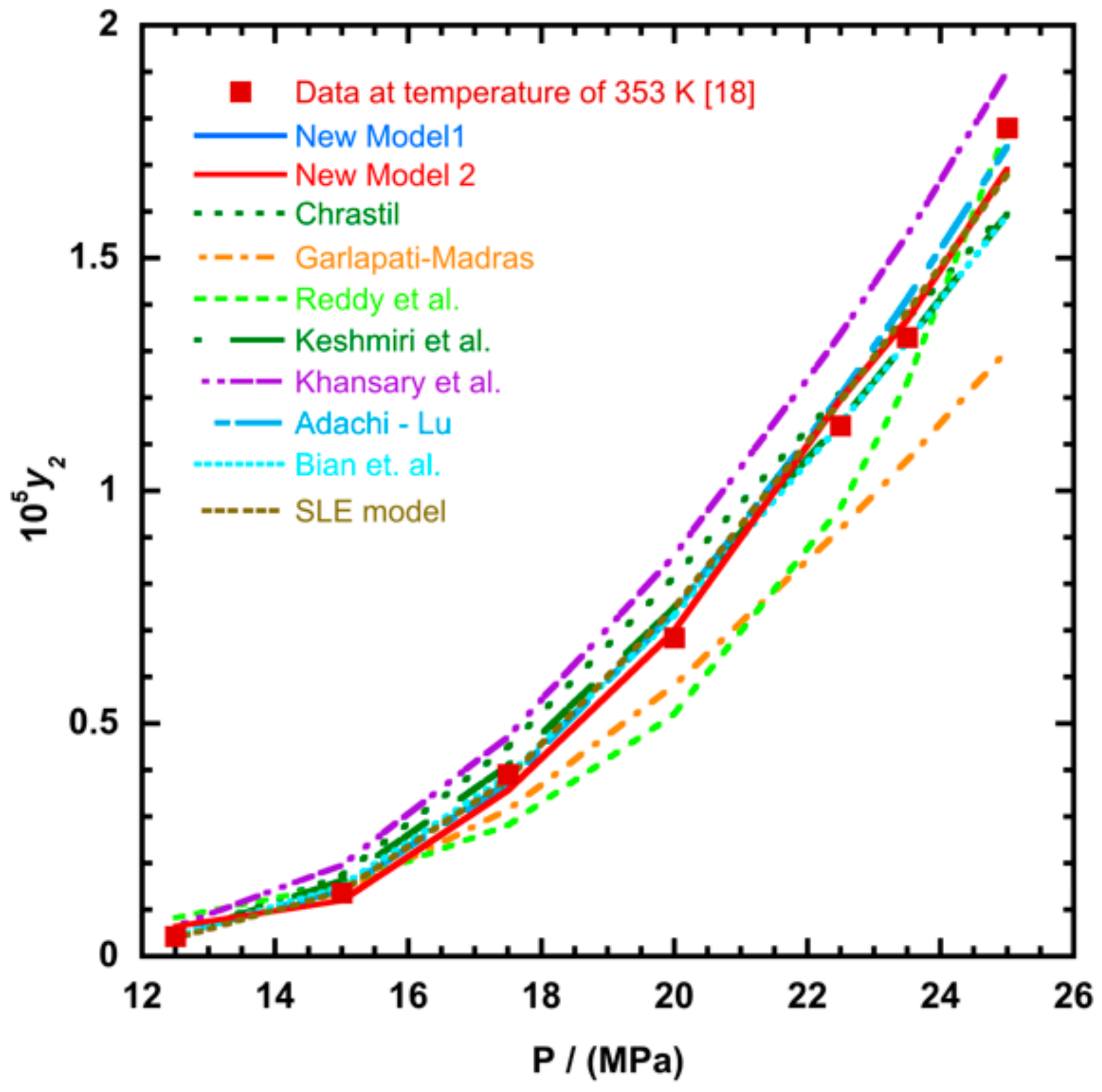
6. Conclusions
Supplementary Materials
Author Contributions
Funding
Data Availability Statement
Acknowledgments
Conflicts of Interest
References
- Gupta, R.B.; Shim, J.-J. Solubility in Supercritical Carbon Dioxide, 1st ed.; CRC Press: Boca Raton, FL, USA, 2007; ISBN 1420005995. [Google Scholar]
- Garlapati, C.; Madras, G. New empirical expressions to correlate solubilities of solids in supercritical carbon dioxide. Thermochim. Acta 2010, 500, 123–127. [Google Scholar] [CrossRef]
- Sodeifian, G.; Garlapati, C.; Hazaveie, S.M.; Sodeifian, F. Solubility of 2,4,7-Triamino-6-phenylpteridine (Triamterene, Diuretic Drug) in Supercritical Carbon Dioxide: Experimental Data and Modeling. J. Chem. Eng. Data 2020, 65, 4406–4416. [Google Scholar] [CrossRef]
- Alwi, R.S.; Tamura, K. Measurement and Correlation of Derivatized Anthraquinone Solubility in Supercritical Carbon Dioxide. J. Chem. Eng. Data 2015, 60, 3046–3052. [Google Scholar] [CrossRef]
- Kramer, A.; Thodos, G. Solubility of 1-hexadecanol and palmitic acid in supercritical carbon dioxide. J. Chem. Eng. Data 1988, 33, 230–234. [Google Scholar] [CrossRef]
- Iwai, Y.; Koga, Y.; Fukuda, T.; Arai, Y. Correlation of Solubilities of High-Boiling Components in Supercritical Carbon Dioxide Using a Solution Model. J. Chem. Eng. Jpn. 1992, 25, 757–760. [Google Scholar] [CrossRef] [Green Version]
- Su, C.-S.; Chen, Y.-P. Correlation for the solubilities of pharmaceutical compounds in supercritical carbon dioxide. Fluid Phase Equilib. 2007, 254, 167–173. [Google Scholar] [CrossRef]
- Chrastil, J. Solubility of solids and liquids in supercritical gases. J. Phys. Chem. 1982, 86, 3016–3021. [Google Scholar] [CrossRef]
- Sridar, R.; Bhowal, A.; Garlapati, C. A new model for the solubility of dye compounds in supercritical carbon dioxide. Thermochim. Acta 2013, 561, 91–97. [Google Scholar] [CrossRef]
- Adachi, Y.; Lu, B.C.-Y. Supercritical fluid extraction with carbon dioxide and ethylene. Fluid Phase Equilib. 1983, 14, 147–156. [Google Scholar] [CrossRef]
- Mitra, S.; Wilson, N.K. An Empirical Method to Predict Solubility in Supercritical Fluids. J. Chromatogr. Sci. 1991, 29, 305–309. [Google Scholar] [CrossRef]
- Keshmiri, K.; Vatanara, A.; Yamini, Y. Development and evaluation of a new semi-empirical model for correlation of drug solubility in supercritical CO2. Fluid Phase Equilib. 2014, 363, 18–26. [Google Scholar] [CrossRef]
- Asgarpour Khansary, M.; Amiri, F.; Hosseini, A.; Hallaji Sani, A.; Shahbeig, H. Representing solute solubility in supercritical carbon dioxide: A novel empirical model. Chem. Eng. Res. Des. 2015, 93, 355–365. [Google Scholar] [CrossRef]
- Bian, X.-Q.; Zhang, Q.; Du, Z.-M.; Chen, J.; Jaubert, J.-N. A five-parameter empirical model for correlating the solubility of solid compounds in supercritical carbon dioxide. Fluid Phase Equilib. 2016, 411, 74–80. [Google Scholar] [CrossRef]
- Reddy, T.A.; Srividya, R.; Garlapati, C. A new empirical model to correlate solubility of pharmaceutical compounds in supercritical carbon dioxide. J. Appl. Sci. Eng. Methodol. 2018, 4, 575–590. [Google Scholar]
- Alwi, R.S.; Tanaka, T.; Tamura, K. Measurement and correlation of solubility of anthraquinone dyestuffs in supercritical carbon dioxide. J. Chem. Thermodyn. 2014, 74. [Google Scholar] [CrossRef]
- Tamura, K.; Alwi, R.S.; Tanaka, T.; Shimizu, K. Solubility of 1-aminoanthraquinone and 1-nitroanthraquinone in supercritical carbon dioxide. J. Chem. Thermodyn. 2017, 104. [Google Scholar] [CrossRef]
- Tamura, K.; Alwi, R.S. Solubility of anthraquinone derivatives in supercritical carbon dioxide. Dye. Pigment. 2015, 113. [Google Scholar] [CrossRef]
- Tamura, K.; Fukamizu, T. Representation of solubilities of phenylthioanthraquinone in supercritical carbon dioxide using Hansen solubility parameter. Fluid Phase Equilib. 2019, 489, 68–74. [Google Scholar] [CrossRef]
- Jain, A.; Yang, G.; Yalkowsky, S.H. Estimation of Melting Points of Organic Compounds. Ind. Eng. Chem. Res. 2004, 43, 7618–7621. [Google Scholar] [CrossRef] [Green Version]
- Fedors, R.F. A method for estimating both the solubility parameters and molar volumes of liquids. Polym. Eng. Sci. 1974, 14, 147–154. [Google Scholar] [CrossRef]
- Giddings, J.C.; Myers, M.N.; McLaren, L.; Keller, R.A. High Pressure Gas Chromatography of Nonvolatile Species. Science 1968, 162, 67–73. [Google Scholar] [CrossRef] [PubMed]
- National Institute of Standards and Technology. U.S. Department of Commerce. Available online: https://webbook.nist.gov/chemistry (accessed on 28 September 2020).
- Prausnitz, J.M.; Lichtenthaler, R.N.; de Azvedo, E.G. Molecular Thermodynamics of Fluid-Phase Equilibria, 3rd ed.; Prentice-Hall: Upper Saddle River, NJ, USA, 1999. [Google Scholar]
- Nordström, F.L.; Rasmuson, Å.C. Solubility and Melting Properties of Salicylic Acid. J. Chem. Eng. Data 2006, 51, 1668–1671. [Google Scholar] [CrossRef]
- Kramer, A.; Thodos, G. Adaptation of the Flory-Huggins theory for modeling supercritical solubilities of solids. Ind. Eng. Chem. Res. 1988, 27, 1506–1510. [Google Scholar] [CrossRef]
- Lee, J.W.; Min, J.M.; Bae, H.K. Solubility Measurement of Disperse Dyes in Supercritical Carbon Dioxide. J. Chem. Eng. Data 1999, 44, 684–687. [Google Scholar] [CrossRef]
- Lagarias, J.C.; Reeds, J.A.; Wright, M.H.; Wright, P.E. Convergence Properties of the Nelder—Mead Simplex Method in Low Dimensions. SIAM J. Optim. 1998, 9, 112–147. [Google Scholar] [CrossRef] [Green Version]
- Reddy, T.A.; Garlapati, C. Dimensionless Empirical Model to Correlate Pharmaceutical Compound Solubility in Supercritical Carbon Dioxide. Chem. Eng. Technol. 2019, 42, 2621–2630. [Google Scholar] [CrossRef]
- Akaike, H. Likelihood of a model and information criteria. J. Econom. 1981, 16, 3–14. [Google Scholar] [CrossRef]
- Akaike, H. A New Look at the Statistical Model Identification. IEEE Trans. Automat. Contr. 1974, 19, 716–723. [Google Scholar] [CrossRef]
- Joung, S.N.; Shin, H.Y.; Park, Y.H.; Yoo, K.-P. Measurement and correlation of solubility of disperse anthraquinone and azo dyes in supercritical carbon dioxide. Korean J. Chem. Eng. 1998, 15, 78–84. [Google Scholar] [CrossRef]
- Lee, J.W.; Park, M.W.; Bae, H.K. Measurement and correlation of dye solubility in supercritical carbon dioxide. Fluid Phase Equilib. 2000, 173, 277–284. [Google Scholar] [CrossRef]
- Coelho, J.P.; Stateva, R.P. Solubility of red 153 and blue 1 in supercritical carbon dioxide. J. Chem. Eng. Data 2011, 56, 4686–4690. [Google Scholar] [CrossRef]
- Ferri, A.; Banchero, M.; Manna, L.; Sicardi, S. An experimental technique for measuring high solubilities of dyes in supercritical carbon dioxide. J. Supercrit. Fluids 2004, 30, 41–49. [Google Scholar] [CrossRef]
- Fat’hi, M.R.; Yamini, Y.; Sharghi, H.; Shamsipur, M. Solubilities of Some 1,4-Dihydroxy-9,10-anthraquinone Derivatives in Supercritical Carbon Dioxide. J. Chem. Eng. Data 1998, 43, 400–402. [Google Scholar] [CrossRef]
- Shamsipur, M.; Karami, A.R.; Yamini, Y.; Sharghi, H. Solubilities of Some Aminoanthraquinone Derivatives in Supercritical Carbon Dioxide. J. Chem. Eng. Data 2003, 48, 71–74. [Google Scholar] [CrossRef]
- Shamsipur, M.; Karami, A.R.; Yamini, Y.; Sharghi, H. Solubilities of some 1-hydroxy-9,10-anthraquinone derivatives in supercritical carbon dioxide. J. Supercrit. Fluids 2004, 32, 47–53. [Google Scholar] [CrossRef]


| Serial Number & Name | Tm | b (KJ/mol) | v2·104 c (m3/mol) | |
|---|---|---|---|---|
| 1. | C.I. disperse blue 3 | 453.6 a | 35.48 | 2.172 |
| 2. | Blue 1 | 599.74 b | 34.42 | 1.894 |
| 3. | 1,4-dihydroxy-9,10-anthraquinone | 469.15 a | 27.81 | 1.665 |
| 4. | 1-Hydroxy-4-(prop-2-enyloxy)-9,10-anthraquinone | 463.38 b | 31.74 | 2.030 |
| 5. | 1,4-bis(prop-2′-enyloxy)-9,10-anthraquinone | 448.17 b | 35.67 | 2.280 |
| 6. | 1-amino-2-methylanthraquinone | 478.15 a | 24.12 | 1.789 |
| 7. | 1- amino-2-ethyl-9,10-anthraquinone | 427.15 a | 26.95 | 1.732 |
| 8. | 1-amino-2,3-dimethylanthraquinone | 486.15 a | 24.60 | 1.790 |
| 9. | 1-hydroxy-9,10-anthraquinone | 599.28 a | 23.92 | 1.610 |
| 10. | 1-hydroxy-2-methylanthraquinone | 458.15 a | 24.40 | 1.759 |
| 11. | 1-hydroxy-2-(methoxy methyl)anthraquinone | 433.94 b | 29.72 | 1.964 |
| 12. | 1-hydroxyl-2-(ethoxy methyl)anthraquinone | 401.15 a | 32.55 | 2.113 |
| 13. | 1-hydroxy-2-(1-propoxy methyl)anthraquinone | 424.0 b | 35.39 | 2.263 |
| 14. | 1-hydroxy-2-(1-butoxymethyl) anthraquinone | 389.74 b | 38.22 | 2.412 |
| 15. | 1-hydroxy-2-(n-amyloxy methyl) anthraquinone | 418.64 b | 41.06 | 2.561 |
| 16. | Quinizarin | 469.15a | 27.81 | 1.665 |
| 17. | Violet 1(1,4-diaminoanthraquinone) | 539.15 a | 27.23 | 1.178 |
| 18. | Blue 59 (1,4-bis (ethyl amino)anthraquinone) | 471.15 a | 33.04 | 1.880 |
| 19. | Red 15 (1-amino-4-hydroxyanthraquinone) | 489.15 a | 27.51 | 1.116 |
| 20. | 1 hydroxy-4-nitroanthraquinone | 540 a | 26.61 | 1.214 |
| 21 | 1,8-dihidroxy-4,5-dinitroanthraquinone | 573.1 a | 33.19 | 1.254 |
| 22. | 1,4 diamino-2,3-dichloroanthraquinone | 576 a | 29.38 | 1.758 |
| 23. | 1-aminoanthraquinone | 526 a | 23.63 | 1.176 |
| 24. | 1-nitroanthraquinone | 505.5 a | 22.73 | 1.554 |
| 25. | C.I. Disperse orange 11 | 478.15 a | 24.12 | 1.789 |
| Serial Number and Name | Chemical Structure | Solubility Range × 106 | T(K) and P(MPa) Range | N | Reference | |
|---|---|---|---|---|---|---|
| 1. | C.I. disperse blue 3 |  | 0.68–63.575 | (323.7–413.7); (10.51–32.98) | 23 | [33] |
| 2. | Blue 1 |  | 6.63–44.5 | (333.3–373.2); (20–40) | 18 | [34] |
| 3. | 1,4-dihydroxy-9,10-anthraquinone |  | 13–314 | (308–348); (12.16–40.53) | 40 | [35,36] |
| 4. | 1-Hydroxy-4-(prop-2′-enyloxy)-9,10-anthraquinone |  | 9–498 | (308–348); (12.16–40.53) | 38 | [36] |
| 5. | 1,4-bis(prop-2′-enyloxy)-9,10-anthraquinone |  | 2–200 | (308–348); (12.16–40.53) | 34 | [36] |
| 6. | 1-amino-2-methylanthraquinone |  | 4.6–109.6 | (308–348); (12.2–35.5) | 43 | [37] |
| 7. | 1- amino-2-ethyl-9,10-anthraquinone |  | 2.6–77.8 | (308–348); (12.2–35.5) | 43 | [37] |
| 8. | 1-amino-2,3-dimethylanthraquinone |  | 4.6–37.9 | (308–348); (12.2–35.5) | 41 | [37] |
| 9. | 1-hydroxy-9,10-anthraquinone |  | 30–445 | (308–348); (12.2–35.5) | 45 | [38] |
| 10. | 1-hydroxy-2-methylanthraquinone |  | 9–737 | (308–348); (12.2–35.5) | 45 | [38] |
| 11. | 1-hydroxy-2-(methoxy methyl)anthraquinone |  | 1–537 | (308–348); (12.2–35.5) | 45 | [38] |
| 12. | 1-hydroxyl-2-(ethoxy methyl)anthraquinone |  | 23–1100 | (308–348); (12.2–35.5) | 45 | [38] |
| 13. | 1-hydroxy-2-(1-propoxy methyl)anthraquinone |  | 103–1676 | (308–348); (12.2–35.5) | 45 | [38] |
| 14. | 1-hydroxy-2-(1-butoxymethyl) anthraquinone |  | 82–2699 | (308–348); (12.2–35.5) | 45 | [38] |
| 15. | 1-hydroxy-2-(n-amyloxy methyl) anthraquinone |  | 38–2640 | (308–348); (12.2–35.5) | 45 | [38] |
| 16. | Quinizarin |  | 69–6940 | (353.2–393.2); (12–30) | 15 | [35,36] |
| 17. | Violet 1(1,4-diaminoanthraquinone) |  | 0.13–2.61 | (323.15–383.15); (15–25) | 15 | [16] |
| 18. | Blue 59 (1,4-bis (ethyl amino)anthraquinone) |  | 0.218–14.9 | (323.15–383.15); (12.5–25) | 26 | [16] |
| 19. | Red 15 (1-amino-4-hydroxyanthraquinone) |  | 1.84–24.5 | (323.15–383.15); (12.5–25) | 20 | [18] |
| 20. | 1 hydroxy-4-nitroanthraquinone |  | 1.22–8.64 | (323.15–383.15); (15–25) | 15 | [18] |
| 21 | 1,8-dihidroxy-4,5-dinitroanthraquinone |  | 0.168–1.12 | (323.15–383.15); (15–25) | 15 | [4] |
| 22. | 1,4 diamino-2,3-dichloroanthraquinone |  | 0.053–5.24 | (323.15–383.15); (12.5–25) | 18 | [4] |
| 23. | 1-aminoanthraquinone |  | 0.55–35.1 | (323.15–383.15); (12.5–25) | 18 | [17] |
| 24. | 1-nitroanthraquinone |  | 0.984–25.2 | (323.15–383.15); (12.5–25) | 18 | [17] |
| 25. | C.I. Disperse orange 11 |  | 0.58–30.3 | (323.15–383.15); (12–25) | 12 | [32] |
| Sl.No* | a | b | c | AARD% |
|---|---|---|---|---|
| 1 | 16,983 | 0.111170 | 1.15140 | 55.328 |
| 2 | 14,423 | 8.083700 | 0.76039 | 34.399 |
| 3 | 14,867 | 0.524320 | 1.01780 | 12.935 |
| 4 | 13,786 | 0.390040 | 1.04700 | 14.982 |
| 5 | 15,545 | 0.025248 | 1.30360 | 36.224 |
| 6 | 14,282 | 1.375900 | 0.92731 | 16.165 |
| 7 | 17,441 | 0.022117 | 1.31830 | 25.785 |
| 8 | 19,195 | 0.002538 | 1.52380 | 23.006 |
| 9 | 13,508 | 0.477910 | 1.03180 | 12.740 |
| 10 | 16,683 | 0.021064 | 1.32190 | 8.198 |
| 11 | 15,754 | 0.000044 | 1.97910 | 82.871 |
| 12 | 13,395 | 0.693360 | 0.99182 | 18.228 |
| 13 | 13,574 | 0.153700 | 1.13460 | 16.541 |
| 14 | 10,512 | 2.867000 | 0.86305 | 17.309 |
| 15 | 13,936 | 0.081591 | 1.18840 | 36.363 |
| 16 | 16,800 | 0.000017 | 2.01370 | 32.140 |
| 17 | 22,206 | 0.000122 | 1.59150 | 39.940 |
| 18 | 18,628 | 0.010357 | 1.38690 | 8.268 |
| 19 | 22,846 | 0.009591 | 1.38010 | 6.304 |
| 20 | 22,936 | 0.001514 | 1.56360 | 11.761 |
| 21 | 23,417 | 0.001591 | 1.55150 | 28.828 |
| 22 | 19,181 | 0.005504 | 1.45030 | 14.566 |
| 23 | 22,218 | 0.002795 | 1.50580 | 5.625 |
| 24 | 18,613 | 0.096199 | 1.17250 | 10.777 |
| 25 | 18,221 | 0.010624 | 1.39170 | 20.698 |
| Sl.No* | A12 | A21·105 | N1 | N2 | N3 | AARD% | R2 | Adj.R2 | RMSE·107 | SSE·1016 |
|---|---|---|---|---|---|---|---|---|---|---|
| 1 | 4.6317 | 7.4408 | −123.220 | 5849.4 | 16.501 | 10.3260 | 0.925 | 0.904 | 30.93 | 2,295,600 |
| 2 | 3.6237 | 0.1369 | −22.280 | 491.4 | 1.197 | 1.2124 | 0.998 | 0.997 | 0.04 | 2.85400 |
| 3 | 3.8856 | 56.018 | −119.110 | 5355.7 | 16.390 | 4.3482 | 0.980 | 0.977 | 76.09 | 23,159,000 |
| 4 | 4.1249 | 66.839 | −255.500 | 11861.0 | 36.544 | 7.8210 | 0.802 | 0.773 | 185.89 | 138,230,000 |
| 5 | 4.4232 | 34.492 | 352.360 | −17338.0 | −53.119 | 7.8357 | 0.905 | 0.891 | 96.46 | 37,222,000 |
| 6 | 3.9076 | 20.069 | −35.941 | 1222.0 | 4.032 | 4.6621 | 0.949 | 0.943 | 28.25 | 3,592,400 |
| 7 | 4.3202 | 11.976 | −44.086 | 1418.5 | 5.251 | 5.8040 | 0.941 | 9.340 | 29.90 | 4,023,100 |
| 8 | 3.7536 | 10.665 | −133.510 | 5959.7 | 18.268 | 2.3299 | 0.981 | 0.979 | 6.39 | 183,520 |
| 9 | 3.7520 | 100.30 | −65.421 | 2831.4 | 8.549 | 2.5184 | 0.960 | 0.954 | 66.34 | 19,807,000 |
| 10 | 4.1139 | 100.84 | −118.880 | 5233.1 | 16.522 | 8.1326 | 0.945 | 0.938 | 308.08 | 427,110,000 |
| 11 | 3.6917 | 132.15 | −81.270 | 3572.1 | 10.940 | 8.1276 | 0.843 | 0.823 | 309.64 | 431,440,000 |
| 12 | 3.8667 | 183.28 | −54.582 | 2282.9 | 7.074 | 4.9246 | 0.960 | 0.955 | 300.20 | 405,550,000 |
| 13 | 3.8025 | 327.28 | −73.225 | 3236.9 | 9.889 | 3.6837 | 0.963 | 0.958 | 333.17 | 499,500,000 |
| 14 | 4.0108 | 399.95 | −203.750 | 9484.9 | 29.170 | 6.1019 | 0.964 | 0.960 | 825.19 | 3,064,200,000 |
| 15 | 4.2943 | 294.42 | −80.585 | 3362.6 | 11.087 | 9.7765 | 0.919 | 0.909 | 1267.30 | 7,226,900,000 |
| 16 | 4.8875 | 1186.7 | 967.570 | −52133.0 | −140.540 | 11.4640 | 0.906 | 0.867 | 8137.90 | 119,200,000,000 |
| 17 | 3.8754 | 0.4939 | −95.533 | 4234.2 | 12.097 | 4.6045 | 0.946 | 0.924 | 0.66 | 657.72 |
| 18 | 4.2476 | 2.0376 | −114.860 | 5180.0 | 15.189 | 10.5440 | 0.967 | 0.960 | 6.82 | 139,560 |
| 19 | 4.1111 | 3.8448 | −141.350 | 6609.0 | 19.113 | 8.9540 | 0.922 | 0.879 | 9.75 | 199,440 |
| 20 | 3.7799 | 1.8628 | −78.114 | 3418.2 | 9.746 | 3.1992 | 0.993 | 0.989 | 1.63 | 3990.60 |
| 21 | 3.5828 | 0.3210 | −31.261 | 922.3 | 2.662 | 1.1563 | 0.973 | 0.958 | 0.10 | 13.78 |
| 22 | 4.3364 | 0.5898 | −148.990 | 6728.0 | 20.046 | 10.9930 | 0.891 | 0.831 | 2.82 | 14339 |
| 23 | 4.1502 | 4.8759 | −128.930 | 5935.5 | 17.365 | 9.4322 | 0.903 | 0.848 | 14.82 | 395,570 |
| 24 | 3.9199 | 4.3919 | −67.609 | 2866.9 | 8.373 | 5.3605 | 0.977 | 0.965 | 7.33 | 96,592 |
| 25 | 4.3723 | 3.6415 | 28.875 | −2317.9 | −5.576 | 10.1480 | 0.970 | 0.953 | 16.25 | 316,930 |
| Sl.No* | A12 | A21·105 | A | B | C·10−5 | AARD/% | R2 | Adj.R2 | RMSE·1012 | SSE·106 |
|---|---|---|---|---|---|---|---|---|---|---|
| 1 | 4.6319 | 7.461 | −1.0778 | −6194.3 | 10.941 | 10.347 | 0.925 | 0.904 | 229.99000 | 3.0956 |
| 2 | 3.6237 | 0.137 | −13.461 | −353.46 | 0.744 | 1.2124 | 1.000 | 1.000 | 0.00029 | 0.0040 |
| 3 | 3.8855 | 56.020 | 0.35304 | −5347.8 | 8.728 | 4.3504 | 0.980 | 0.977 | 2319.70 | 7.6153 |
| 4 | 4.1251 | 66.837 | 10.906 | −12028 | 19.499 | 7.8214 | 0.947 | 0.940 | 13855.00 | 18.6110 |
| 5 | 4.4208 | 34.554 | −34.627 | 17225 | −28.081 | 7.8227 | 0.905 | 0.891 | 3719.90 | 9.6436 |
| 6 | 3.9077 | 20.070 | −6.642 | −1350.7 | 2.048 | 4.6627 | 0.949 | 0.943 | 360.00 | 2.8284 |
| 7 | 4.3203 | 11.977 | −5.9057 | −1950 | 2.697 | 5.8043 | 0.941 | 0.934 | 403.16 | 2.9932 |
| 8 | 3.7542 | 10.660 | −0.2361 | −6047.9 | 9.856 | 2.3265 | 0.981 | 0.979 | 18.39 | 0.6393 |
| 9 | 3.752 | 100.310 | −3.0674 | −2776.4 | 4.593 | 2.5168 | 0.961 | 0.956 | 1983.30 | 6.6387 |
| 10 | 4.114 | 100.850 | 1.5165 | −5534 | 8.762 | 8.1321 | 0.945 | 0.938 | 42,770.00 | 30.8290 |
| 11 | 3.7153 | 120.250 | 0.29924 | −4765.9 | 7.677 | 4.0867 | 0.984 | 0.982 | 2753.40 | 7.8222 |
| 12 | 3.8668 | 183.240 | −2.9085 | −2409.6 | 3.886 | 4.9225 | 0.960 | 0.954 | 40,519 | 30.0070 |
| 13 | 3.8026 | 327.230 | −1.0388 | −3291.2 | 5.381 | 3.6796 | 0.963 | 0.958 | 49,885 | 33.2950 |
| 14 | 4.0108 | 400.240 | 8.7869 | −9511.2 | 15.448 | 6.1073 | 0.965 | 0.960 | 307,640 | 82.6830 |
| 15 | 4.2944 | 294.450 | −0.13121 | −3641.3 | 5.518 | 9.7817 | 0.919 | 0.909 | 725,400 | 126.960 |
| 16 | 4.8875 | 1186.800 | −75.478 | 52,674 | −97.606 | 11.464 | 0.906 | 0.867 | 11,919,000 | 813.740 |
| 17 | 3.8754 | 0.494 | −6.4227 | −4295.6 | 7.500 | 4.6045 | 0.946 | 0.916 | 0.06577 | 0.0662 |
| 18 | 4.2476 | 2.038 | −2.9703 | −5529.4 | 9.416 | 10.544 | 0.967 | 0.960 | 13.9560 | 0.6820 |
| 19 | 4.1111 | 3.845 | −0.55598 | −6866.1 | 11.846 | 8.954 | 0.922 | 0.896 | 19.9440 | 0.9745 |
| 20 | 3.7799 | 1.863 | −6.3245 | −3452.8 | 6.041 | 3.1992 | 0.993 | 0.989 | 0.39906 | 0.1631 |
| 21 | 3.5828 | 0.321 | −11.654 | −954.12 | 1.649 | 1.1563 | 0.973 | 0.958 | 0.00138 | 0.0096 |
| 22 | 4.3364 | 0.590 | −1.3261 | −7404.6 | 12.425 | 10.993 | 0.891 | 0.846 | 1.43390 | 0.2823 |
| 23 | 4.1502 | 4.876 | −1.0106 | −6311.3 | 10.770 | 9.4324 | 0.903 | 0.862 | 39.5560 | 1.4824 |
| 24 | 3.9199 | 4.392 | −5.9336 | −3036 | 5.190 | 5.3605 | 0.977 | 0.968 | 9.65920 | 0.7326 |
| 25 | 4.3723 | 3.642 | −12.201 | 1613.4 | −3.456 | 10.148 | 0.970 | 0.945 | 31.6930 | 1.6251 |
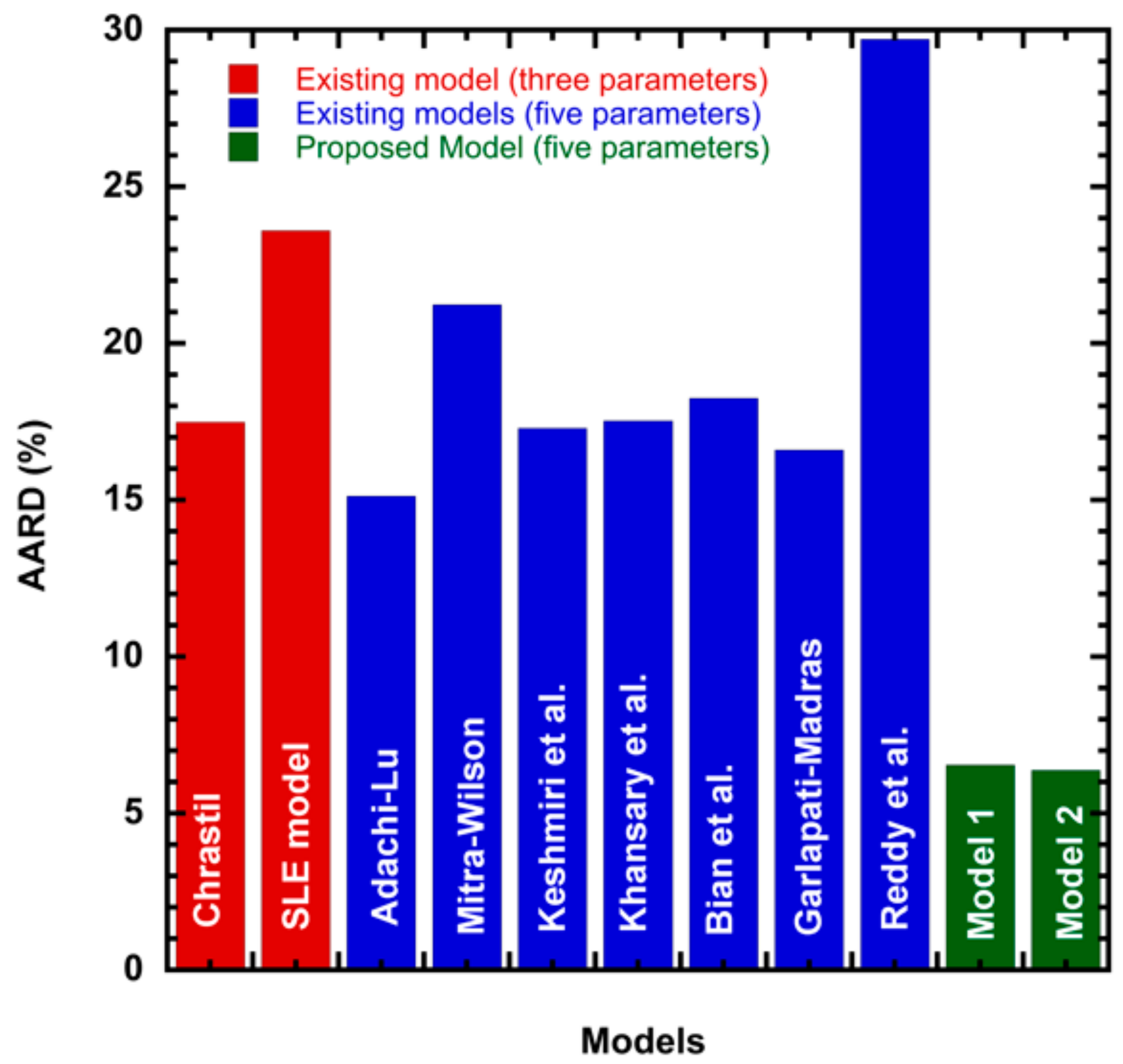
| Model | No. of Constants | R2 | Adj. R2 | SSE | RMSE | AARD % |
|---|---|---|---|---|---|---|
| Chrastil | 3 | 0.89690 | 0.89295 | 1.30 −6 | 1.01 −4 | 17.485 |
| Adachi-Lu | 5 | 0.89850 | 0.89780 | 1.27 | 7.69 −2 | 15.130 |
| Mitra-Wilson | 5 | 0.87990 | 0.87560 | 3.539 | 1.70 −1 | 21.240 |
| Keshmiri et al. | 5 | 0.89100 | 0.35800 | 2.75 −7 | 1.00 −4 | 17.298 |
| Khansary et al. | 5 | 0.89100 | 0.88700 | 6.67 −7 | 6.24 −5 | 17.530 |
| Bian et al. | 5 | 0.89644 | 0.89278 | 2.69 −7 | 4.97 −5 | 18.251 |
| Garlapati-Madras | 5 | 0.87800 | 0.87300 | 2.01 −7 | 4.53 −5 | 16.599 |
| Reddy et al. | 5 | 0.75600 | 0.74400 | 3.92 −6 | 1.50 −4 | 29.711 |
| SLE model | 3 | 0.88985 | 0.86064 | 4.44 −6 | 1.77 −4 | 23.599 |
| New Model 1 | 5 | 0.93930 | 0.92270 | 5.26 −7 | 4.825 −5 | 6.538 |
| New Model 2 | 5 | 0.95092 | 0.93728 | 4.73 −4 | 5.244 −7 | 6.377 |
| Paired t-test Results for AARD, R2 and Adj.R2 | ||||||
| Models | AARD | R2 | Adj. R2 | |||
| New Model 1 | New Model 2 | New Model 1 | New Model 2 | New Model 1 | New Model 2 | |
| Chrastil | S | S | NS | NS | NS | NS |
| Adachi-Lu | S | S | NS | NS | NS | NS |
| Mitra-Wilson | S | S | S | S | NS | NS |
| Keshmiri et al. | S | S | NS | NS | NS | NS |
| Khansary et al. | S | S | S | S | S | NS |
| Bian et al. | S | S | NS | NS | NS | NS |
| Garlapati-Madras | S | S | S | S | NS | NS |
| Reddy et al. | S | S | S | S | NS | S |
| SLE model | S | S | S | S | NS | NS |
| Paired t-test Results for SSE and RMSE | ||||||
| Models | SSE | RMSE | ||||
| New Model 1 | New Model 2 | New Model 1 | New Model 2 | |||
| Chrastil | NS | NS | NS | NS | ||
| Adachi-Lu | NS | NS | S | NS | ||
| Mitra-Wilson | NS | NS | S | S | ||
| Keshmiri et al. | NS | NS | NS | NS | ||
| Khansary et al. | NS | NS | S | NS | ||
| Bian et al. | NS | NS | NS | NS | ||
| Garlapati-Madras | NS | NS | NS | NS | ||
| Reddy et al. | NS | NS | NS | NS | ||
| SLE model | NS | NS | NS | NS | ||
| Sl.No* | Equation (18) | Equation (21) | Equation (2) | Equation (3) | Equation (4) | Equation (5) | Equation (6) | Equation (7) | Equation (8) | Equation (9) | SLE (Equations (10)−(12)) |
|---|---|---|---|---|---|---|---|---|---|---|---|
| 1 | −572.60 | −883.48 | −543.41 | −547.95 | −544.26 | −529.96 | −533.91 | −548.37 | −521.14 | −520.16 | −502.02916 |
| 2 | −686.29 | −804.56 | −604.41 | −296.42 | −285.04 | −603.40 | −608.51 | −587.68 | −602.21 | −583.75 | −577.05251 |
| 3 | −932.89 | −1530.00 | −968.16 | −303.79 | −230.96 | −975.80 | −948.67 | −929.28 | −880.29 | −824.08 | −904.08437 |
| 4 | −815.91 | −1417.10 | −711.57 | −53.04 | −44.02 | −700.99 | −706.31 | −693.52 | −698.85 | −672.92 | −692.25585 |
| 5 | −769.80 | −1285.45 | −730.70 | −140.86 | −99.47 | −731.25 | −724.22 | −704.18 | −716.47 | −677.58 | −656.16322 |
| 6 | −1086.85 | −1691.20 | −1051.84 | −326.98 | −284.62 | −1041.34 | −1035.41 | −1010.52 | −1017.78 | −951.70 | −999.79284 |
| 7 | −1081.98 | −1688.77 | −1001.05 | −257.98 | −232.93 | −1006.04 | −1001.16 | −1009.39 | −999.11 | −945.54 | −960.43326 |
| 8 | −1155.83 | −1671.09 | −1022.17 | −331.42 | −313.68 | −1020.25 | −1035.60 | −1005.96 | −977.98 | −980.62 | −1008.7995 |
| 9 | −1063.09 | −1733.98 | −973.50 | −220.08 | −210.03 | −954.59 | −955.82 | −973.06 | −975.24 | −894.61 | −974.00663 |
| 10 | −924.90 | −1664.88 | −970.35 | −215.20 | −156.93 | −961.05 | −951.72 | −929.51 | −928.08 | −832.69 | −975.57241 |
| 11 | −924.44 | −1726.60 | −815.67 | −760.86 | −930.34 | −820.67 | −943.42 | −811.84 | −808.04 | −986.59 | −921.64403 |
| 12 | −927.23 | −1666.10 | −913.68 | −153.10 | −143.13 | −916.41 | −889.74 | −923.98 | −887.23 | −849.04 | −900.93092 |
| 13 | −917.85 | −1661.42 | −876.78 | −128.34 | −80.13 | −883.27 | −875.88 | −866.40 | −821.62 | −790.88 | −871.09925 |
| 14 | −836.22 | −1620.49 | −815.23 | −26.09 | −22.74 | −795.27 | −789.52 | −795.24 | −845.10 | −743.41 | −815.42235 |
| 15 | −797.61 | −1601.19 | −790.56 | −791.01 | −764.98 | −787.64 | −774.85 | −789.17 | −793.49 | −732.22 | −773.78737 |
| 16 | −200.68 | −482.72 | −218.20 | −189.25 | 25.92 | −216.10 | −196.21 | −217.34 | −223.00 | −170.32 | −202.70016 |
| 17 | −485.91 | −623.97 | −270.41 | −234.37 | −238.65 | −486.03 | −469.66 | −494.58 | −491.75 | −463.79 | −173.59318 |
| 18 | −724.58 | −1042.54 | −758.18 | −324.42 | −304.19 | −729.89 | −732.67 | −755.40 | −699.79 | −705.83 | −763.27385 |
| 19 | −542.68 | −787.26 | −265.77 | −241.05 | −228.48 | −547.15 | −532.15 | −545.48 | −514.00 | −533.35 | −569.89688 |
| 20 | −458.87 | −610.44 | −438.25 | −182.81 | −199.53 | −429.90 | −419.25 | −456.83 | −432.72 | −433.09 | −441.6821 |
| 21 | −543.89 | −652.93 | −485.64 | −245.06 | −236.68 | −470.10 | −480.91 | −486.40 | −479.42 | −481.78 | −467.63919 |
| 22 | −532.90 | −727.94 | −559.09 | −248.76 | −247.35 | −538.41 | −527.98 | −556.60 | −539.48 | −528.07 | −570.46594 |
| 23 | −473.19 | −698.09 | −472.09 | −182.95 | −178.74 | −459.60 | −456.90 | −486.09 | −446.49 | −435.79 | −486.12245 |
| 24 | −498.56 | −710.77 | −485.77 | −195.10 | −185.25 | −475.73 | −471.13 | −497.48 | −476.43 | −481.84 | −505.23963 |
| 25 | −309.92 | −456.09 | −303.97 | −110.80 | −97.41 | −298.57 | −295.69 | −298.64 | −275.30 | −287.64 | −295.23155 |
| Overall | −730.59 | −1177.56 | −681.86 | −268.31 | −249.34 | −695.18 | −694.29 | −694.92 | −682.04 | −660.29 | −680.36 |
| Sl.No* | N1 | N2 | N3 | Tm (K) a | |
|---|---|---|---|---|---|
| 1 | −123.22 | 5849.4 | 16.501 | 140.5761 | 46,711.00 |
| 2 | −22.28 | 491.4 | 1.197 | 26.78756 | 3976.00 |
| 3 | −119.11 | 5355.7 | 16.39 | 140.8947 | 42,620.00 |
| 4 | −255.5 | 11861 | 36.544 | 181.0266 | 94,055.00 |
| 5 | 352.36 | −17338 | −53.119 | NA | NA |
| 6 | −35.941 | 1222 | 4.032 | 63.66784 | 9723.90 |
| 7 | −44.086 | 1418.5 | 5.251 | 63.68529 | 11,226.00 |
| 8 | −133.51 | 5959.7 | 18.268 | 136.2973 | 47,423.00 |
| 9 | −65.421 | 2831.4 | 8.549 | 113.3441 | 22,545.00 |
| 10 | −118.88 | 5233.1 | 16.522 | 140.9835 | 41,585.00 |
| 11 | −81.27 | 3572.1 | 10.94 | 125.9199 | 28,425.00 |
| 12 | −54.582 | 2282.9 | 7.074 | 105.5913 | 18,215.00 |
| 13 | −73.225 | 3236.9 | 9.889 | 128.3756 | 25,761.00 |
| 14 | −203.75 | 9484.9 | 29.17 | 183.3302 | 75,220.00 |
| 15 | −80.585 | 3362.6 | 11.087 | 123.8086 | 26,666.00 |
| 16 | 967.57 | −52133 | −140.54 | NA | NA |
| 17 | −95.533 | 4234.2 | 12.097 | 109.262 | 33,795.00 |
| 18 | −114.86 | 5180 | 15.189 | 124.6076 | 41,299.00 |
| 19 | −141.35 | 6609 | 19.113 | 141.5514 | 52,723.00 |
| 20 | −78.114 | 3418.2 | 9.746 | 104.079 | 27,366.00 |
| 21 | −31.261 | 922.3 | 2.662 | 43.4634 | 7402.40 |
| 22 | −148.99 | 6728 | 20.046 | 131.4074 | 53,603.00 |
| 23 | −128.93 | 5935.5 | 17.365 | 136.1121 | 47,327.00 |
| 24 | −67.609 | 2866.9 | 8.373 | 98.16466 | 22,930.00 |
| 25 | 28.875 | −2317.9 | −5.576 | NA | NA |
Publisher’s Note: MDPI stays neutral with regard to jurisdictional claims in published maps and institutional affiliations. |
© 2021 by the authors. Licensee MDPI, Basel, Switzerland. This article is an open access article distributed under the terms and conditions of the Creative Commons Attribution (CC BY) license (http://creativecommons.org/licenses/by/4.0/).
Share and Cite
Alwi, R.S.; Garlapati, C.; Tamura, K. Solubility of Anthraquinone Derivatives in Supercritical Carbon Dioxide: New Correlations. Molecules 2021, 26, 460. https://doi.org/10.3390/molecules26020460
Alwi RS, Garlapati C, Tamura K. Solubility of Anthraquinone Derivatives in Supercritical Carbon Dioxide: New Correlations. Molecules. 2021; 26(2):460. https://doi.org/10.3390/molecules26020460
Chicago/Turabian StyleAlwi, Ratna Surya, Chandrasekhar Garlapati, and Kazuhiro Tamura. 2021. "Solubility of Anthraquinone Derivatives in Supercritical Carbon Dioxide: New Correlations" Molecules 26, no. 2: 460. https://doi.org/10.3390/molecules26020460