
The Role of Structural Representation in the Performance of a Deep Neural Network for X-ray Spectroscopy


Abstract
:1. Introduction
2. Theory and Computational Details
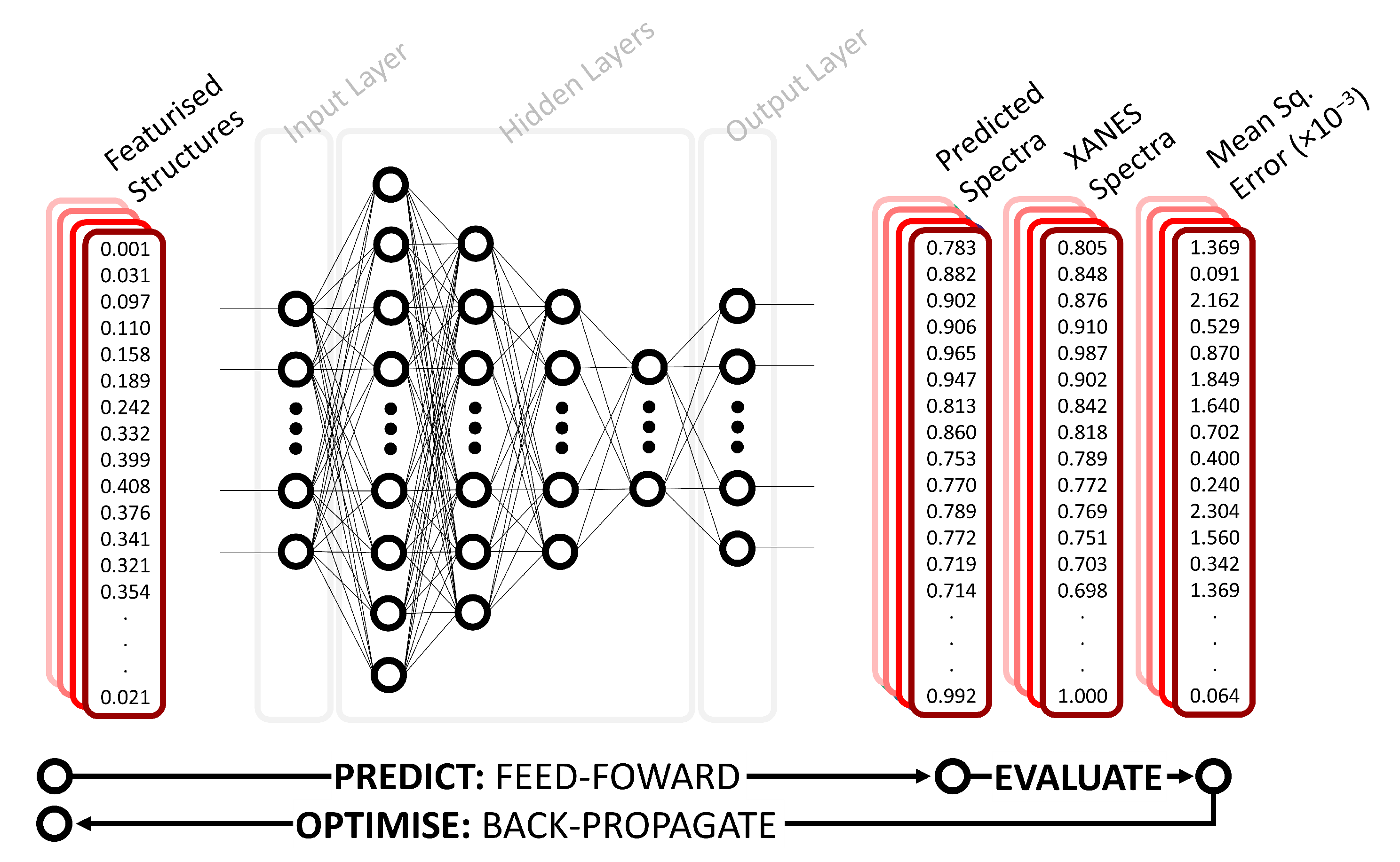
2.1. Deep Neural Network
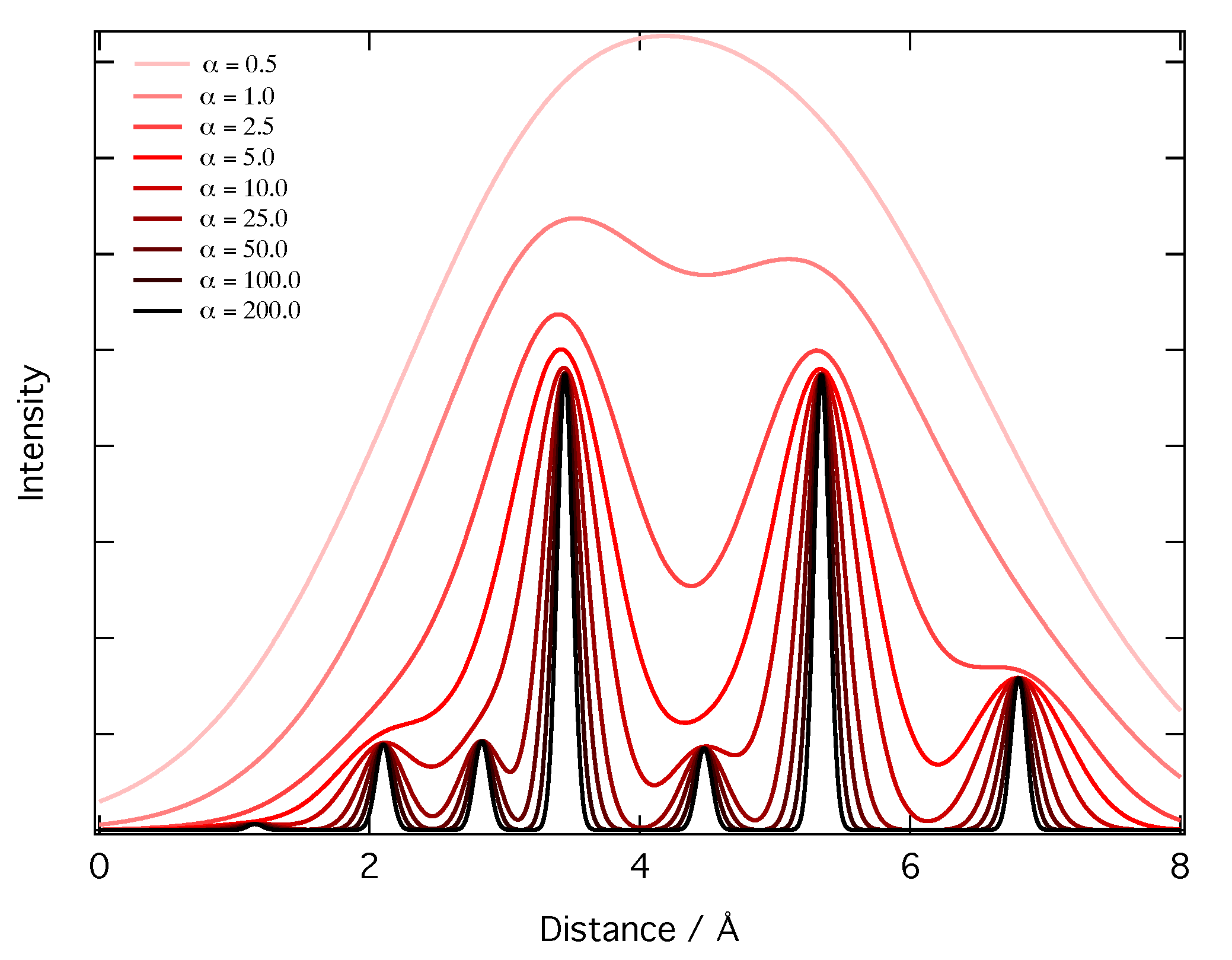
2.2. Representation
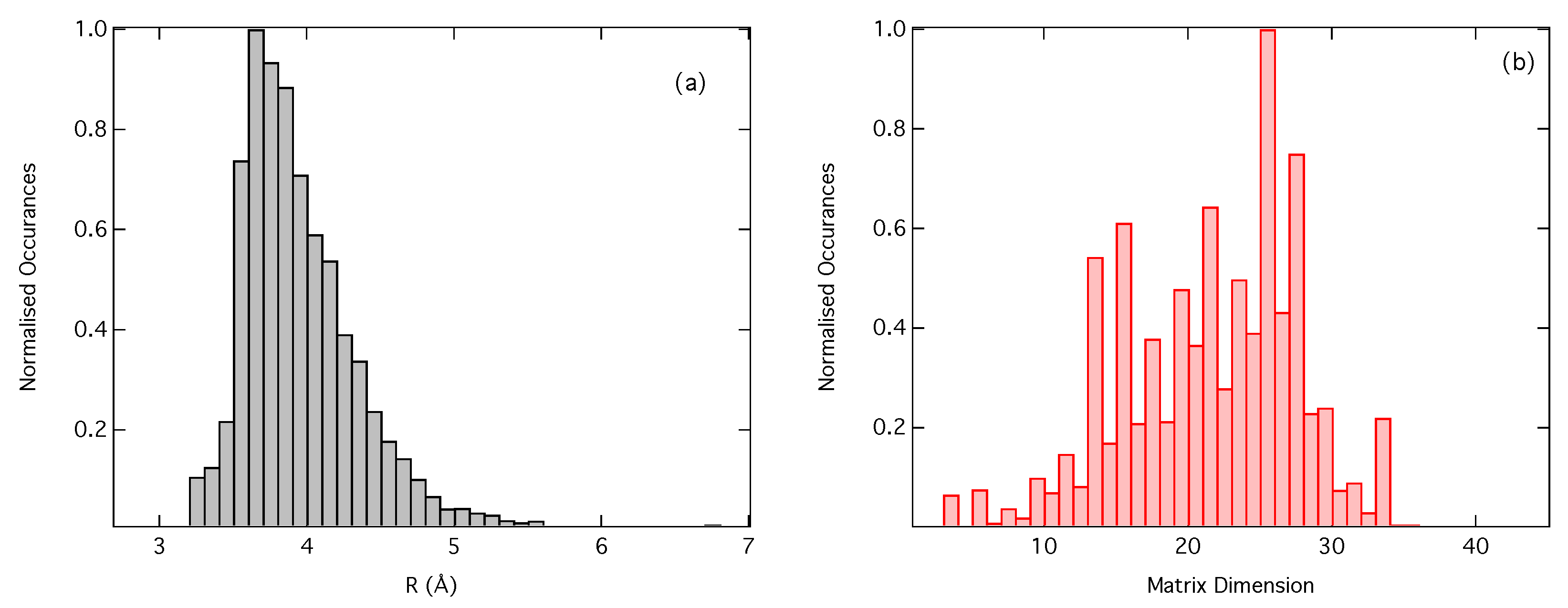
2.3. Dataset
3. Results
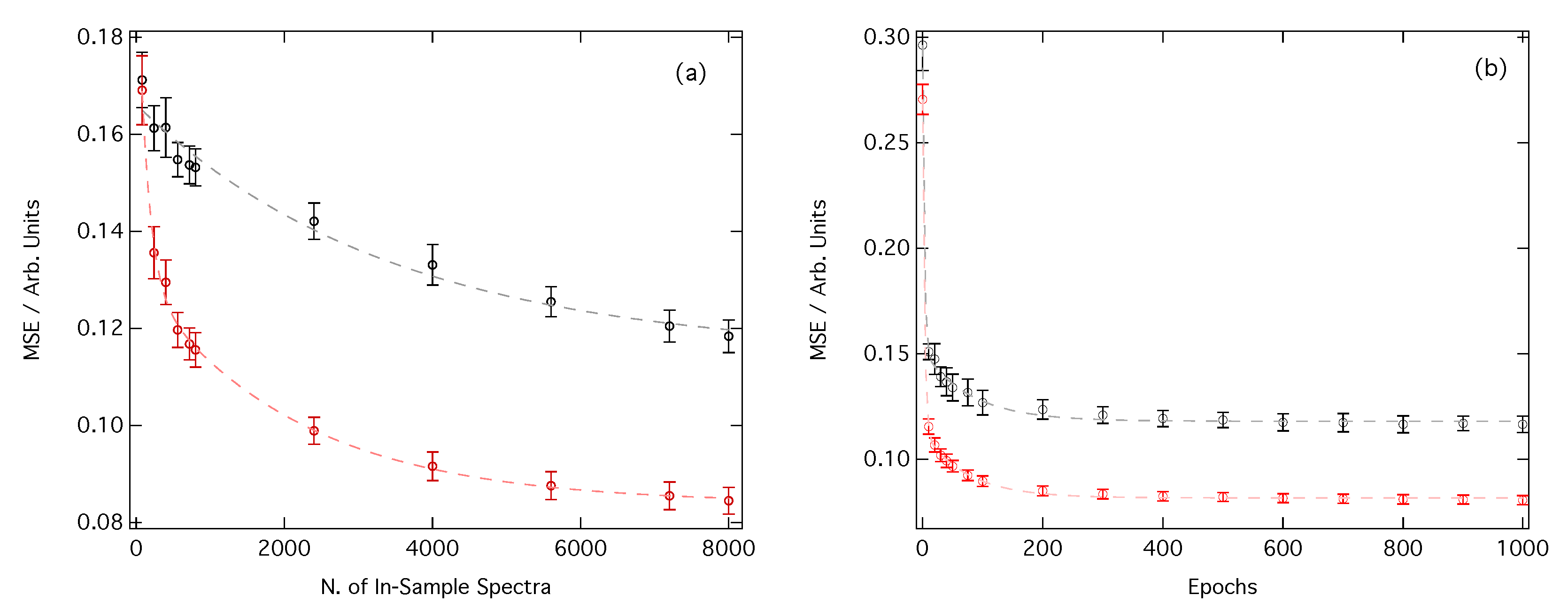
3.1. Performance of the Deep Neural Network
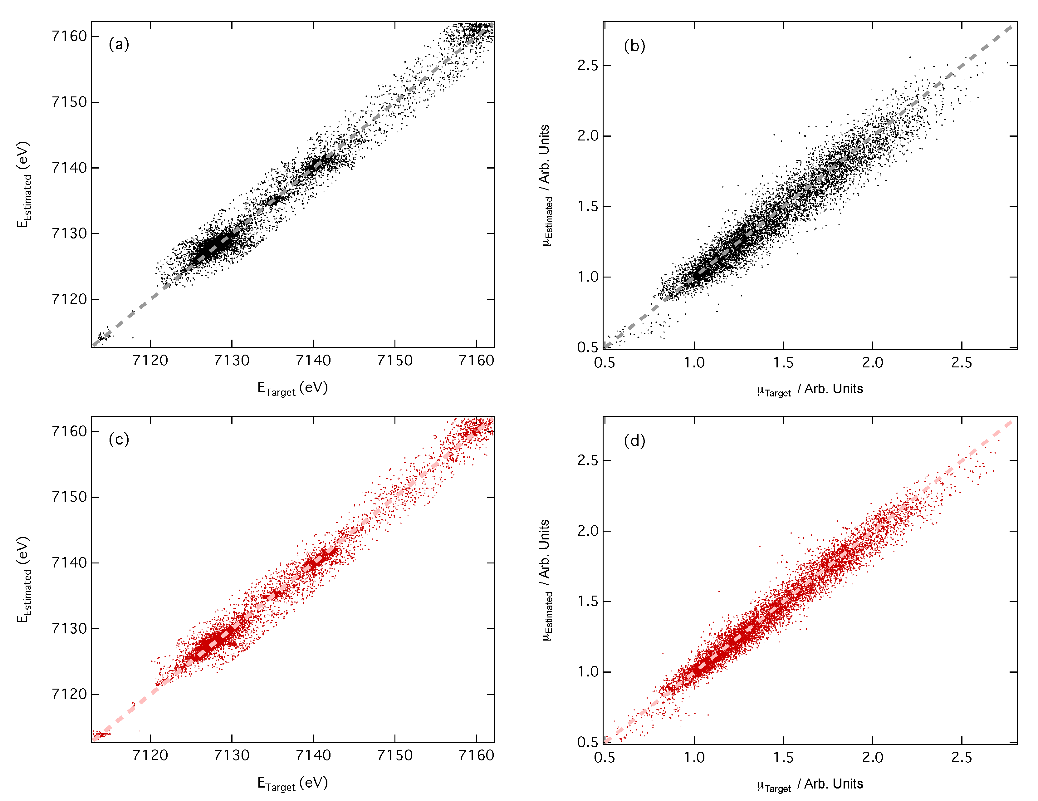
3.2. Predictions of Peak Position and Intensity
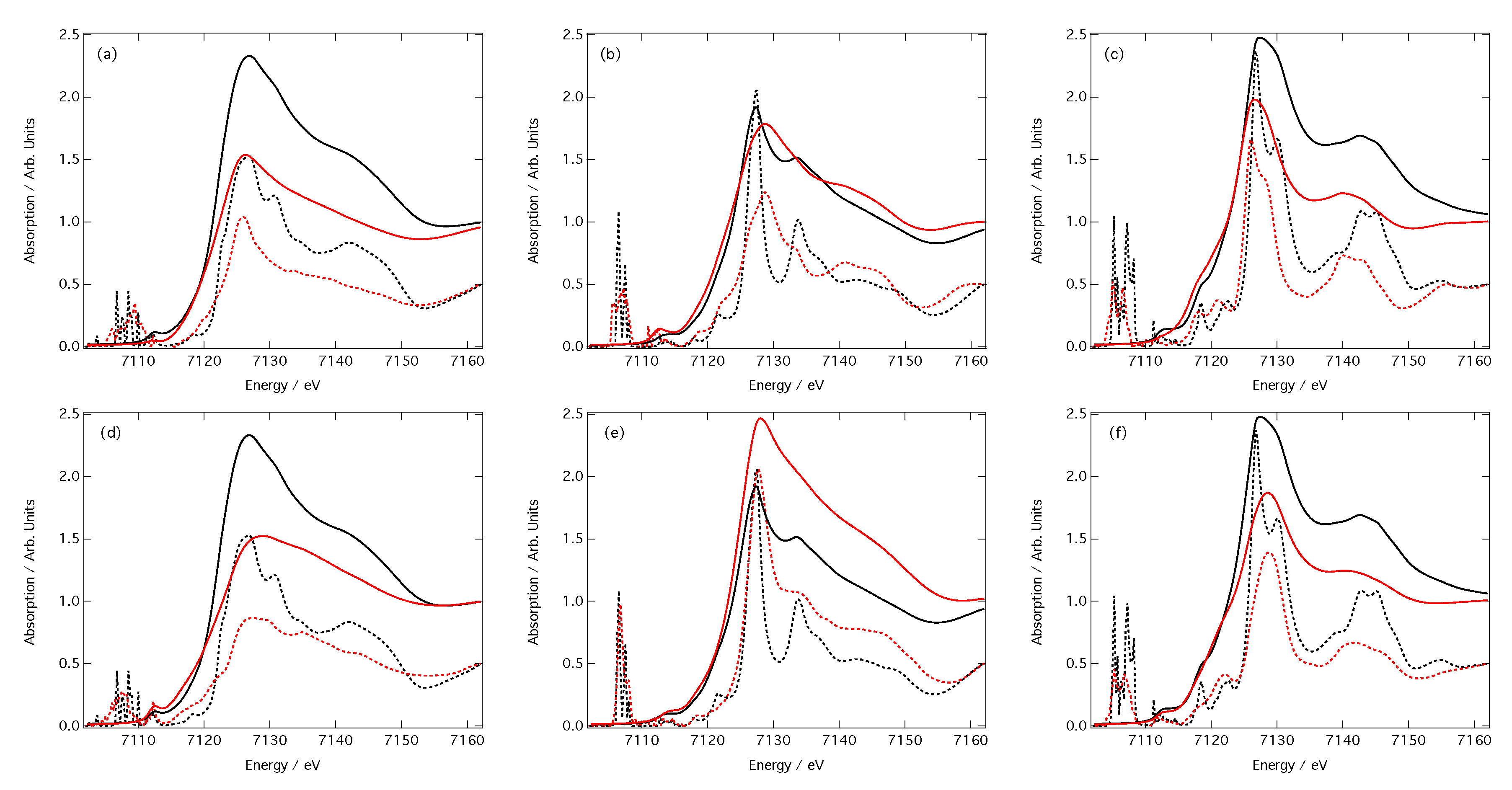
3.3. Predictions of Spectra
4. Discussion and Conclusions
Author Contributions
Funding
Conflicts of Interest
References
- Asakura, H.; Hosokawa, S.; Ina, T.; Kato, K.; Nitta, K.; Uera, K.; Uruga, T.; Miura, H.; Shishido, T.; Ohyama, J.; et al. Dynamic Behavior of Rh Species in a Rh/Al2O3 Model Catalyst During a Three-Way Catalytic Reaction: An Operando X-ray Absorption Spectroscopy Study. J. Am. Chem. Soc. 2018, 140, 176–184. [Google Scholar] [CrossRef]
- Fabbri, E.; Abbott, D.F.; Nachtegaal, M.; Schmidt, T.J. Operando X-ray Absorption Spectroscopy: A Powerful Tool Toward Water-Splitting Catalyst Development. Curr. Opin. Electrochem. 2017, 5, 20–26. [Google Scholar] [CrossRef]
- Penfold, T.; Milne, C.; Chergui, M. Recent Advances in Ultrafast X-ray Absorption Spectroscopy of Solutions. Adv. Chem. Phys. 2013, 153, 1–41. [Google Scholar]
- Milne, C.; Penfold, T.; Chergui, M. Recent Experimental and Theoretical Developments in Time-Resolved X-ray Spectroscopies. Coord. Chem. Rev. 2014, 277, 44–68. [Google Scholar] [CrossRef]
- Koningsberger, D.; Prins, R. X-ray Absorption: Principles, Applications, and Techniques of EXAFS, SEXAFS, and XANES; Wiley: Chichester, UK, 1988. [Google Scholar]
- Bunker, G. Introduction to XAFS: A Practical Guide to X-ray Absorption Fine Structure Spectroscopy; Cambridge University Press: Cambridge, UK, 2010. [Google Scholar]
- Ankudinov, A.; Ravel, B.; Rehr, J.; Conradson, S. Real-Space Multiple-Scattering Calculation and Interpretation of X-ray Absorption Near-Edge Structure. Phys. Rev. B 1998, 58, 7565. [Google Scholar] [CrossRef] [Green Version]
- Rehr, J.J.; Albers, R.C. Theoretical Approaches to X-ray Absorption Fine Structure. Rev. Mod. Phys. 2000, 72, 621. [Google Scholar] [CrossRef]
- O’day, P.; Rehr, J.; Zabinsky, S.; Brown, G.J. Extended X-ray Absorption Fine Structure (EXAFS) Analysis of Disorder and Multiple Scattering in Complex Crystalline Solids. J. Am. Chem. Soc. 1994, 116, 2938–2949. [Google Scholar] [CrossRef]
- Mustre, J.; Yacoby, Y.; Stern, E.A.; Rehr, J.J. Analysis of Experimental Extended X-ray Absorption Fine Structure (EXAFS) Data Using Calculated Curved-Wave, Multiple-Scattering EXAFS Spectra. Phys. Rev. B 1990, 42, 10843. [Google Scholar] [CrossRef]
- Rehr, J.; Ankudinov, A. Progress in the Theory and Interpretation of XANES. Coord. Chem. Rev. 2005, 249, 131–140. [Google Scholar] [CrossRef]
- Bunău, O.; Joly, Y. Self-Consistent Aspects of X-ray Absorption Calculations. J. Phys. Condens. Matter 2009, 21, 345501. [Google Scholar] [CrossRef]
- Kas, J.J.; Jorissen, K.; Rehr, J.J. Real-Space Multiple-Scattering Theory of X-ray Spectra. In X-ray Absorption and X-ray Emission Spectroscopy: Theory and Applications; John Wiley & Sons: Hoboken, NJ, USA, 2016. [Google Scholar]
- Zhou, Y.; Doronkin, D.E.; Zhao, Z.; Plessow, P.N.; Jelic, J.; Detlefs, B.; Pruessmann, T.; Studt, F.; Grunwaldt, J.D. Photothermal Catalysis over Nonplasmonic Pt/TiO2 Studied by Operando HERFD-XANES, Resonant XES, and DRIFTS. ACS Catal. 2018, 8, 11398–11406. [Google Scholar] [CrossRef]
- Hu, H.; Wachs, I.E.; Bare, S.R. Surface Structures of Supported Molybdenum Oxide Catalysts: Characterization by Raman and Mo L3-Edge XANES. J. Phys. Chem. 1995, 99, 10897–10910. [Google Scholar] [CrossRef]
- Alayon, E.M.; Nachtegaal, M.; Ranocchiari, M.; van Bokhoven, J.A. Catalytic Conversion of Methane to Methanol Over Cu Mordenite. Chem. Commun. 2012, 48, 404–406. [Google Scholar] [CrossRef]
- Capano, G.; Milne, C.; Chergui, M.; Rothlisberger, U.; Tavernelli, I.; Penfold, T. Probing Wavepacket Dynamics Using Ultrafast X-ray Spectroscopy. J. Phys. B At. Mol. Opt. Phys. 2015, 48, 214001. [Google Scholar] [CrossRef]
- Penfold, T.J.; Szlachetko, J.; Santomauro, F.G.; Britz, A.; Gawelda, W.; Doumy, G.; March, A.M.; Southworth, S.H.; Rittmann, J.; Abela, R.; et al. Revealing Hole Trapping in Zinc Oxide Nanoparticles by Time-Resolved X-ray Spectroscopy. Nat. Commun. 2018, 9, 478. [Google Scholar] [CrossRef]
- Northey, T.; Norell, J.; Fouda, A.E.; Besley, N.A.; Odelius, M.; Penfold, T.J. Ultrafast Nonadiabatic Dynamics Probed by Nitrogen K-edge Absorption Spectroscopy. Phys. Chem. Chem. Phys. 2020, 22, 2667–2676. [Google Scholar] [CrossRef]
- Hayes, D.; Hadt, R.G.; Emery, J.D.; Cordones, A.A.; Martinson, A.B.; Shelby, M.L.; Fransted, K.A.; Dahlberg, P.D.; Hong, J.; Zhang, X.; et al. Electronic and Nuclear Contributions to Time-Resolved Optical and X-ray Absorption Spectra of Hematite and Insights into Photoelectrochemical Performance. Energy Environ. Sci. 2016, 9, 3754–3769. [Google Scholar] [CrossRef] [Green Version]
- Cannelli, O.; Bacellar, C.; Ingle, R.; Bohinc, R.; Kinschel, D.; Bauer, B.; Ferreira, D.; Grolimund, D.; Mancini, G.; Chergui, M. Toward Time-Resolved Laser T-Jump/X-ray Probe Spectroscopy in Aqueous Solutions. Struct. Dyn. 2019, 6, 064303. [Google Scholar] [CrossRef]
- Kuzmin, A.; Timoshenko, J.; Kalinko, A.; Jonane, I.; Anspoks, A. Treatment of Disorder Effects in X-Ray Absorption Spectra Beyond the Conventional Approach. Radiat. Phys. Chem. 2018. [Google Scholar] [CrossRef] [Green Version]
- Timoshenko, J.; Lu, D.; Lin, Y.; Frenkel, A.I. Supervised Machine-Learning-Based Determination of Three-Dimensional Structure of Metallic Nanoparticles. J. Phys. Chem. Lett. 2017, 8, 5091–5098. [Google Scholar] [CrossRef]
- Timoshenko, J.; Halder, A.; Yang, B.; Seifert, S.; Pellin, M.J.; Vajda, S.; Frenkel, A.I. Subnanometer Substructures in Nanoassemblies Formed from Clusters under a Reactive Atmosphere Revealed Using Machine Learning. J. Phys. Chem. C 2018, 122, 21686–21693. [Google Scholar] [CrossRef]
- Timoshenko, J.; Ahmadi, M.; Cuenya, B.R. Is There a Negative Thermal Expansion in Supported Metal Nanoparticles? An in Situ X-ray Absorption Study Coupled with Neural Network Analysis. J. Phys. Chem. C 2019, 123, 20594–20604. [Google Scholar] [CrossRef] [Green Version]
- Ahmadi, M.; Timoshenko, J.; Behafarid, F.; Cuenya, B.R. Tuning the Structure of Pt Nanoparticles through Support Interactions: An in Situ Polarized X-ray Absorption Study Coupled with Atomistic Simulations. J. Phys. Chem. C 2019, 123, 10666–10676. [Google Scholar] [CrossRef] [PubMed] [Green Version]
- Timoshenko, J.; Wrasman, C.J.; Luneau, M.; Shirman, T.; Cargnello, M.; Bare, S.R.; Aizenberg, J.; Friend, C.M.; Frenkel, A.I. Probing Atomic Distributions in Mono- and Bimetallic Nanoparticles by Supervised Machine Learning. Nano Lett. 2019, 19, 520–529. [Google Scholar] [CrossRef] [PubMed]
- Timoshenko, J.; Frenkel, A.I. “Inverting” X-ray Absorption Spectra of Catalysts by Machine Learning in Search for Activity Descriptors. ACS Catal. 2019, 9, 10192–10211. [Google Scholar] [CrossRef]
- Liu, Y.; Marcella, N.; Timoshenko, J.; Halder, A.; Yang, B.; Kolipaka, L.; Pellin, M.J.; Seifert, S.; Vajda, S.; Liu, P.; et al. Mapping XANES Spectra on Structural Descriptors of Copper Oxide Clusters Using Supervised Machine Learning. J. Chem. Phys. 2019, 151, 164201. [Google Scholar] [CrossRef]
- Carbone, M.R.; Yoo, S.; Topsakal, M.; Lu, D. Classification of Local Chemical Environments from X-ray Absorption Spectra Using Supervised Machine Learning. Phys. Rev. Mater. 2019, 3, 033604. [Google Scholar] [CrossRef]
- Carbone, M.R.; Topsakal, M.; Lu, D.; Yoo, S. Machine-Learning X-Ray Absorption Spectra to Quantitative Accuracy. Phys. Rev. Lett. 2020, 124, 156401. [Google Scholar] [CrossRef] [Green Version]
- Rankine, C.D.; Madkhali, M.M.; Penfold, T.J. A Deep Neural Network for the Rapid Prediction of X-ray Absorption Spectra. J. Phys. Chem. A 2020, 124, 4263–4270. [Google Scholar] [CrossRef] [PubMed]
- Rupp, M.; Tkatchenko, A.; Müller, K.R.; Von Lilienfeld, O.A. Fast and Accurate Modeling of Molecular Atomization Energies with Machine Learning. Phys. Rev. Lett. 2012, 108, 058301. [Google Scholar] [CrossRef] [PubMed]
- Montavon, G.; Rupp, M.; Gobre, V.; Vazquez-Mayagoitia, A.; Hansen, K.; Tkatchenko, A.; Müller, K.R.; Von Lilienfeld, O.A. Learning Invariant Representations of Molecules for Atomization Energy Prediction. In Advances in Neural Information Processing Systems; Pereira, F., Burges, C.J.C., Bottou, L., Weinberger, K.Q., Eds.; Curran Associates Inc.: Red Hook, NY, USA, 2012; Volume 25, pp. 440–448. [Google Scholar]
- Montavon, G.; Rupp, M.; Gobre, V.; Vazquez-Mayagoitia, A.; Hansen, K.; Tkatchenko, A.; Müller, K.R.; Von Lilienfeld, O.A. Machine Learning of Molecular Electronic Properties in Chemical Compound Space. New J. Phys. 2013, 15, 095003. [Google Scholar] [CrossRef]
- Gasteiger, J.; Schuur, J.; Selzer, P.; Steinhauer, L.; Steinhauer, V. Finding the 3D Structure of a Molecule in its IR Spectrum. Fresenius J. Anal. Chem. 1997, 359, 50–55. [Google Scholar] [CrossRef]
- Hemmer, M.C.; Steinhauer, V.; Gasteiger, J. Deriving the 3D Structure of Organic Molecules from their Infrared Spectra. J. Vib. Spectrosc. 1999, 19, 151–164. [Google Scholar] [CrossRef]
- Hemmer, M.C.; Gasteiger, J. Prediction of Three-Dimensional Molecular Structures using Information from Infrared Spectra. Anal. Chim. Acta 2000, 420, 145–154. [Google Scholar] [CrossRef]
- Von Lilienfeld, O.A.; Ramakrishnan, R.; Rupp, M.; Knoll, A. Fourier Series of Atomic Radial Distribution Functions: A Molecular Fingerprint for Machine Learning Models of Quantum Chemical Properties. Int. J. Quantum Chem. 2015, 115, 1084–1093. [Google Scholar] [CrossRef] [Green Version]
- Hansen, K.; Montavon, G.; Biegler, F.; Fazli, S.; Rupp, M.; Scheffler, M.; Von Lilienfeld, O.A.; Tkatchenko, A.; Müller, K.R. Assessment and Validation of Machine Learning Methods for Predicting Molecular Atomization Energies. J. Chem. Theory Comput. 2013, 9, 3404–3419. [Google Scholar] [CrossRef]
- Hinton, G.E.; Srivastava, N.; Krizhevsky, A.; Sutskever, I.; Salakhutdinov, R.R. Improving Neural Networks by Preventing Co-Adaptation of Feature Detectors. arXiv 2012, arXiv:1207.0580. [Google Scholar]
- Abadi, M.; Agarwal, A.; Barham, P.; Brevdo, E.; Chen, Z.; Citro, C.; Corrado, G.S.; Davis, A.; Dean, J.; Devin, M.; et al. TensorFlow: Large-Scale Machine Learning on Heterogeneous Distributed Systems. Available online: http://tensorflow.org/ (accessed on 11 June 2020).
- Keras. 2015. Available online: http://github.com/keras-team/keras (accessed on 11 June 2020).
- GPy: A Gaussian Process Framework in Python. 2012. Available online: http://github.com/SheffieldML/GPy (accessed on 11 June 2020).
- GPyOpt: A Bayesian Optimization Framework in Python. 2016. Available online: http://github.com/SheffieldML/GPyOpt (accessed on 11 June 2020).
- Fernandez, M.; Trefiak, N.R.; Woo, T.K. Atomic-Property-Weighted Radial Distribution Functions Descriptors of Metal–Organic Frameworks for the Prediction of Gas Uptake Capacity. J. Phys. Chem. C 2013, 27, 14095–14105. [Google Scholar] [CrossRef]
- Krykunov, M.; Woo, T.K. Bond-Type-Restricted Property-Weighted Radial Distribution Functions for Accurate Machine Learning Prediction of Atomization Energies. J. Chem. Theory Comput. 2018, 14, 5229–5237. [Google Scholar] [CrossRef]
- Seah, M.; Dench, W. NPL Report Chem. 1978, 82, 1.
- Reinhard, M.; Penfold, T.; Lima, F.; Rittmann, J.; Rittmann-Frank, M.; Abela, R.; Tavernelli, I.; Rothlisberger, U.; Milne, C.; Chergui, M. Photooxidation and Photoaquation of Iron Hexacyanide in Aqueous Solution: A Picosecond X-ray Absorption Study. Struct. Dyn. 2014, 1, 024901. [Google Scholar] [CrossRef] [PubMed]
- Penfold, T.J.; Karlsson, S.; Capano, G.; Lima, F.A.; Rittmann, J.; Reinhard, M.; Rittmann-Frank, M.; Bräm, O.; Baranoff, E.; Abela, R.; et al. Solvent-Induced Luminescence Quenching: Static and Time-Resolved X-ray Absorption Spectroscopy of a Copper(I) Phenanthroline Complex. J. Phys. Chem. A 2013, 117, 4591–4601. [Google Scholar] [CrossRef] [PubMed]
Sample Availability: Samples of the compounds are not available from the authors. |


© 2020 by the authors. Licensee MDPI, Basel, Switzerland. This article is an open access article distributed under the terms and conditions of the Creative Commons Attribution (CC BY) license (http://creativecommons.org/licenses/by/4.0/).
Share and Cite
Madkhali, M.M.M.; Rankine, C.D.; Penfold, T.J. The Role of Structural Representation in the Performance of a Deep Neural Network for X-ray Spectroscopy. Molecules 2020, 25, 2715. https://doi.org/10.3390/molecules25112715
Madkhali MMM, Rankine CD, Penfold TJ. The Role of Structural Representation in the Performance of a Deep Neural Network for X-ray Spectroscopy. Molecules. 2020; 25(11):2715. https://doi.org/10.3390/molecules25112715
Chicago/Turabian StyleMadkhali, Marwah M.M., Conor D. Rankine, and Thomas J. Penfold. 2020. "The Role of Structural Representation in the Performance of a Deep Neural Network for X-ray Spectroscopy" Molecules 25, no. 11: 2715. https://doi.org/10.3390/molecules25112715