Article

Pricing Decisions and Coordination in E-Commerce Supply Chain with Wholesale Price Contract Considering Focus Preferences

1
School of Management, Shanghai University, Shanghai 200444, China
2
School of Economics and Management, Shanghai University of Political Science and Law, Shanghai 201701, China
*
Author to whom correspondence should be addressed.
J. Theor. Appl. Electron. Commer. Res. 2023, 18(2), 1041-1068; https://doi.org/10.3390/jtaer18020053
Submission received: 5 April 2023 / Revised: 7 May 2023 / Accepted: 30 May 2023 / Published: 3 June 2023

Abstract

:
Decision makers’ behavioral preferences have always been important in coordinating the supply chain. Decision makers need to choose a partner wisely to increase the profitability of the entire supply chain, especially in the competitive e-commerce environment. In this paper, we examine a two-echelon e-commerce supply chain with one retailer and one supplier using the most popular wholesale price contract to facilitate collaboration. Traditional research has shown that the classical expectation model cannot coordinate the supply chain. We apply the focus theory of choice to describe the retailer’s behavior as a follower, and we examine the impact of the retailer’s pricing decisions on the supplier under different focus preferences and the coordination for the entire supply chain. The lower the parameter φ, which represents the degree of positivity, and the higher the parameter κ, which represents the level of confidence, the closer the profit of the whole supply chain is to the coordination result—both are visualized through numerical experiments and images. In the case of φ determination, the lower the κ, the better the supply chain coordination. The finding implies that the retailer may be able to coordinate the supply chain and produce better results than the expectation model when he or she makes choices using a positive evaluation system that includes both higher levels of optimism and lower levels of confidence. The findings of the FTC model can simultaneously offer a theoretical foundation for expanding collaboration among supply chain participants and management insights for decision makers to choose cooperation partners.

1. Introduction

In the era of e-commerce, the speed of product replacement and life cycle has become shorter, and there are more competing products and substitutes for similar products. Upstream suppliers in the supply chain can increase their competitiveness by setting up direct online sales, while downstream retailers are constantly improving their decision-making flexibility in response to changing market needs. Now many retailers are relying on e-commerce platforms to change their sales model to a pre-order system, retaining operational flexibility to respond to demand information by promising consumers to order in advance while being able to reduce their costs [1]. The supply chain has been transformed from the traditional form based on internal enterprise information to a modern e-commerce supply chain that relies on electronization, intellectualization, and digitization. Current market transactions are based on many e-commerce platforms, and according to official statistics from Taobao, as of January 2023, 26,160,060 shops had been entered. E-commerce platforms include a variety of sales models and can meet the sales needs of multiple categories of merchants and have full applicability to a wide range of supply chains. However, e-commerce supply chains still suffer from the efficiency problems found in traditional supply chains, with decentralized decision-making between subjects leading to double marginalization of utility and reduced system efficiency [2]. Multiple coordination mechanisms in supply chain management remain a very important element in e-commerce supply chain coordination, facilitating supply chain members to coordinate with each other as a whole and maintain the unity of purpose [3,4], which can reduce costs, improve the economic stability of the supply chain, and reduce channel conflicts when the supply chain makes decisions as a whole [5]. The formation of supply chain contracts can further improve the efficient payoff distribution among decision makers as well as the sustainability of the supply chain, indicating that overall coordination is still a key component of business cooperation for e-commerce supply chains.
The decentralized supply chain is coordinated when the order volume of the decentralized supply chain equals the order volume of the centralized supply chain, resulting in the total expected payoff of the decentralized supply chain equaling the total expected payoff of the centralized supply chain [6,7,8]. The most widely applied wholesale price contract provides insights on adjusting decision makers’ target utility to improve overall efficiency. Of course, there are other complex contracts that can coordinate the supply chain, and given the importance of the contract in the coordination mechanism, the very common question is which contract to adopt [9]. The design of cooperative contracts among supply chain members takes into account issues such as supply chain coordination, profit sharing, and the cost of maintaining the contract [10]. Therefore, considering the many influencing factors, the designer of the contract may prefer a wholesale price contract to other complex contracts.
We used the focus theory of choice (FTC) to emphasize the importance of salient information in decisions of uncertainty, and the limited rationality characteristics of individuals based on FTC are more consistent with human behavior patterns in the process of making decisions, consistent with the results of psychological experiments conducted by Stewart [11]. We use FTC to promote coordination, aiming to be similar to the real situation and involve the impact of individuals with different personality traits on coordination. Based on the e-commerce environment and a one-time decision problem, the product market demand is more stochastic, and the uncertainty of demand is an important cause of the pull-to-center effect, which makes the decision deviate from the optimal [12]. Establishing a supply chain contract under a stochastic demand setting considers numerous influencing factors. A number of scholars are currently studying issues such as a demand-dependent two-echelon supply chain with retail price and the impact of variable demand on production, further emphasizing the problem of uncertainty in product demand and proposing some solutions [13,14,15]. Scholars provided supply chain operation insights on the one hand by building new supply chain contracts or applying new behavioral preferences, and on the other, they applied new management strategies to improve management efficiency and production cost-effectiveness [16]. The limitations of human judgment can exacerbate supply chain challenges and even potentially undermine strategic initiatives, highlighting the need to redesign and validate “human factors” to better inform relevant decisions [17].
Below we summarize our contributions. We consider a two-echelon e-commerce supply chain consisting of a single supplier and a single retailer that adopts a wholesale price contract. In the FTC framework, a new supply chain coordination model is developed to analyze the changes in the decision-making of retailers with positive focus preference and the impact on the whole supply chain coordination under the wholesale price contract. Our results show that FTC can coordinate the supply chain and solve the double marginalization effect under certain conditions. The model also provides a theoretical basis for suppliers and retailers to establish further cooperation and offers new theoretical ideas for coordinating the supply chain. The retailer’s FTC-based decision-making behavior allows the overall supply chain profitability to achieve results better than the classical expectation model under many conditions.
The remainder of this paper is organized as follows. Section 2 reviews the literature. In Section 3, we review the classical expectation-based wholesale price contract model in the two-echelon supply chain and the double marginalization problem of the channel as the basis for the focus model. In Section 4, based on the expected value model, we develop a focus model of the retailer’s decision process to find the optimal retail price of the retailer and infer the optimal wholesale price of the supplier’s decision as the dominant player in the face of different retailers’ personality characteristics. In Section 5, give numerical experiments and results. In Section 6, we compare another behavioral model to analyze the supply chain coordination and overall channel payoff change under the positive focus model. Section 7 concludes this paper. Some of the proofs are given in Appendix A.

2. Literature Review

Decision makers’ personalities can have a big impact on how supply chain transactions turn out. The focus theory of choice, which outperforms traditional models and is more in line with the decision-making process of realistic decision makers, is used in this study to assess retailers’ responses. Hence, the related literature review is classified into three areas—(i) supply chain contracts and coordination, (ii) theoretical study on behavioral supply chains, and (iii) study on the focus theory of choice.

2.1. Supply Chain Contracts and Coordination

When establishing cooperation among supply chain members, coordination issues are an important factor to consider. As an example, due to centralized or decentralized supply chain operations, the distribution of finished products for the final process may require different coordination mechanisms. Scholars have proposed a variety of cooperative contract models, such as the most studied wholesale price contract [18], and Holmstrom and Milgrom have long suggested that, in reality, channel members often adopt a simpler collaborative contract [19], so the adoption of wholesale price contracts in the supply chain has many aspects of applicability. Scholars Cachon et al., observed that revenue-sharing contracts have some coordination effect in the video leasing industry [20], and Pasternack demonstrated the coordination of buyback contracts in the newsvendor model [21]. Katok and Wu show that revenue-sharing contracts and buyback contracts are mathematically equivalent in certain settings but do not usually lead to equivalent supply chain performance in practice [22]. Zhang et al., again demonstrate this equivalence from the supply chain perspective [23]. This part of scholars’ research on supply chains focuses on coordination mechanisms, mostly comparing the performance differences between different coordination mechanisms and the issue of equivalence, without considering the influence of behavioral preferences on the final decision outcome.
For e-commerce businesses, the e-commerce clothes industry, the online food fresh category, and many other industries, wholesale price contracts are still commonly employed [24]. Given the complexity of the supply chain, the wholesale price contract is the most popular form of contract [25,26]. Early scholars Bernstein et al., studied supply chain performance through a simple wholesale price contract where suppliers were able to coordinate the supply chain under a specific discount setting [27]. With the development of e-commerce, coordinating the supply chain remains a key issue. Qiu et al., investigated the coordination problem for a two-tier decentralized supply chain consisting of a supplier and a retailer who sells the product both offline and online to consumers with reference quality effect, considering the factors influencing market demand and the impact of supply chain contracts on coordination [28]. Shu et al., consider a supplier selling substituted products to an e-retailer through wholesale selling mode or mixed use of wholesale and agency selling mode (hybrid contracts) [29]. However, the above-mentioned papers continue to concentrate on the issue of creating coordination mechanisms without considering the influence of behavioral preferences on coordination.

2.2. Behavioral Supply Chain

The classical expected utility theory has been continuously applied in operations research-based supply chain models, where fully rational decision makers can coordinate the supply chain through some cooperative contracts [30,31]. With the development of behavioral economics, the Allais paradox and Ellsberg paradox challenged the expected utility theory and the subjective expected utility theory, respectively [32,33]. A growing number of experimental behavioral studies have challenged the “economic man” hypothesis. Experimental results show that a variety of factors, such as market conditions and information differences, influence upstream and downstream decision makers and their actual economic decisions often deviate from predictions based on expected utility maximization [12,34,35,36]. Schweitzer and Cachon found that these decision biases were characterized by a “pull-to-center effect” in the experiment, as the average number of orders was low when it should have been high, and vice versa [12]. Later, Bostian et al., replicated this effect in a laboratory study, and this feature remained very evident in multiple rounds of experiments [37]. The classical expected utility theory has proved to be unable to solve the decision bias in the supply chain, and the behavioral factors are more closely and importantly linked to the supply chain [38].
For better coordination, the role of behavior in the supply chain has become increasingly important [39]. Research has greatly enriched behavioral theories, such as prospect theory and heuristic decision bias, which have corrective and developmental implications for expected utility theory, as well as the study of irrational behavior with perspectives such as fairness concern, psychological accounts, and overconfidence [40,41,42,43,44,45]. Some of these theories have ruled out explanations for the “pull-to-center effect”, such as risk aversion or risk-seeking, loss aversion, and other behavioral theories [12]. Majeed et al., think that behavioral preferences are distinct from economic motivation and will influence behaviors in the supply chain. Decision makers will make decisions based on not only self-interests but also the interests of others, reciprocity, and fairness [46].
Many irrational behavior theories are more biased toward behavioral economics research that ignores the procedural nature of behavioral decisions and have more restrictions in their application to supply chains. The fairness concern theory is only applicable to two- or multi-person settings. Additionally, if the decision maker is independent or does not know the profit composition of the cooperating party, the decision maker with fairness concern has no reference to utility and does not consider the pull-to-center effect in the decision bias phenomenon. Overconfidence is defined as a cognitive bias that cannot fully account for the decision-making process and can only explain a single personality trait.

2.3. The Focus Theory of Choice

FTC was originally proposed by Guo, who believed that human attention is limited and the decision-making process has a certain order, similar to buying a lottery ticket. The decision maker will consider the probability of winning and the prize amount, and people with different personality traits will focus on different probabilities and benefits to obtain the final decision results [47]. This procedure involves two steps: in the first step, for each action, some specific event that can bring about a relatively high payoff with a relatively high probability or a relatively low payoff with a relatively high probability is selected as the positive or negative focus, respectively; in the second step, based on the foci of all actions, a decision maker chooses a most-preferred action [48,49]. FTC handles decision-making with risk or when facing ambiguity or ignorance within a unified framework. Additionally, FTC explains the St. Petersburg paradox, the Allais paradox, and the Ellsberg paradox with the central idea that finite rational decision makers select the salient information (focus) of greatest concern to evaluate various options in events that are more consistent with human decision-making processes in real life. Additionally, salient information plays a crucial role in the decision-making process. Based on FTC, scholars proposed some new approaches to solve stochastic optimization problems [48,50].
Some scholars have used FTC to incorporate decision makers’ personality traits into mathematical models and analyzed the impact of FTC on decisions, supporting the importance of decision makers with different traits for strategic choices [51]. Zhu et al., used FTC to solve the behavioral decision problem in the newsvendor problem and solved for the retailer’s optimal order quantity in the framework of FTC, showing that when a retailer is more optimistic about uncertain demand and more confident in his or her decision, he or she tends to aim high and act more aggressively by ordering a higher quantity [52]. This paper only explores the retailer’s decision in the newsvendor model and does not analyze the impact on the supplier when applied to the supply chain, but it can serve as the basis for this paper on supply chain coordination. Later, a study by Zhu et al., who studied the optimal replenishment of retailers under the vendor-managed inventory model based on FTC, provided a new perspective to analyze the behavior of individual suppliers in a VMI program with revenue-sharing contracts [53]. Zhu et al., studied a two-echelon supply chain under retailer-led buyback contracts in the presence of uncertain market demand, and this paper used FTC to describe the behavioral tendencies of the supplier and to theoretically obtain the optimal wholesale price based on the supplier’s focus preference [54]. These two papers examine revenue-sharing contracts and buyback contracts, respectively, and the emphasis of the papers is on emphasizing differences in decision-making among decision makers with different personality characteristics and the effect of optimism on outcomes, with no following comparison descriptions. The FTC-related papers do not evaluate the impact on supply chain performance or the function of supply chain coordination; instead, they primarily discuss the varied decision outcomes of decision makers with focus preferences under distinct types of personalities. In addition to this, we use the wholesale price contracts to analyze decision outcomes, firstly because the real-life generalizability is a bit stronger, and secondly because the literature studying wholesale price contracts is more extensive and easier to compare with the results of other behavioral preferences.

3. The Classical Model of the Wholesale Price

The classical model studied in this paper consists of a fully rational two-echelon supply chain consisting of a single supplier and a single retailer. Both make decisions according to their expected payoff maximization, and the decentralized decision is made first by the supplier as the dominant player, who sets a wholesale price ( w ) , and then the retailer sets the retail price ( r ) under the given wholesale price. The list of notations used in this study is given in Table 1.
Assume that the market potential demand faced by the product is a random variable, denoted by the capital letter X , has a probability density function f · and obeys a cumulative distribution function F · . The range belongs to the interval l , h ; l denotes the lowest market potential demand, h denotes the highest market potential demand, 0 l h , and μ denotes the expected value of the market potential demand X . The supplier produces at a fixed cost c per unit of production, satisfying the size relationship of 0 < c w r . Additionally, the retailer faces linear uncertainty product demand; D X , r = X b r , where b ( > 0 ) is the sensitivity of product market demand concerning the retail price. The supplier offers a cooperation contract to the retailer, and the retailer either rejects this offer, in which case neither partner makes any payoffs, or orders D X , r units. Since retailers adopt a reservation system in e-commerce platforms, this paper assumes that the retailer’s orders are matched with retail price, only the supplier has unit production cost, and the retailer’s wholesale products can be sold fully without out-of-stock cost (opportunity cost), inventory cost, and salvage value.
The payoff functions of the supplier and retailer are given as follows:
v s r , w , X = w c X b r ,
v r r , w , X = r w X b r .
The whole potential payoff of the supply chain is given as follows:
v r , X = r c X b r ,
where assumes D l , r 0 to ensure that the product market demand is non-negative when the potential market demand takes the lowest value l , i.e., r l b ; assuming w 2 l h b , it is guaranteed that payoff loss may occur when market demand is too high or low.
The expected payoff of the whole supply chain (denoted as V ( r ) ) is given by
V ( r ) = b r 2 + μ + b c r c μ .
whereas b > 0 , it can be judged that the second-order derivative of V ( r ) is negative, i.e., 2 b < 0 . The function V ( r ) is a concave function about r . The maximum point r * = μ + b c 2 b is within the valid interval, and the maximum value of V ( r ) is obtained as V r * = μ b c 2 4 b .
In decentralized decision-making, the retailer’s decision is first analyzed according to the standard inverse induction of the Stackelberg game. Denote the expected payoffs of the retailer and supplier as V r ( r , w ) and V s w . In this case, the retailer’s expected payoff function is given below:
V r ( r , w ) = b r 2 + μ + b w r w μ .
Since r 1 = μ + b w 2 b is the symmetry axis of V r ( r , w ) must be within the valid interval, the optimal expected payoff of the retailer is obtained as V r ( r 1 , w ) = μ b w 2 4 b . The optimal wholesale price of the supplier and the optimal expected payoff is obtained from r as w 1 = μ + b c 2 b and V s w 1 = μ b c 2 8 b . The final outcomes of the retailer are r 1 = 3 μ + b c 4 b and V r r 1 , w 1 = μ b c 2 16 b . At this point, the whole payoff of the supply chain (denoted as V * ( r ) ) is given by
V * ( r ) = V r ( r 1 , w 1 ) + V s w 1 = 3 4 · μ b c 2 4 b .
The sum of the payoffs generated by the supplier and the retailer under the decentralized decision is lower than the optimal payoff under the centralized channel when considering the expected payoff, leading to double marginalization.

4. The Wholesale Price Model with the Positive Focus Theory of Choice

4.1. FTC Model

We analyze the decision-making model of a retailer under a positive evaluation system, assuming that the retailer’s decision-making process is a single-cycle decision that requires a one-time decision on the retail price. When the supplier dominates, the wholesale price is provided first, and the retailer with a positive focus preference decides on the e-commerce platform through a reservation system. Based on the given wholesale price and all potential retail prices, the positive demand focus is determined by comparing the satisfaction and likelihood of potential market demand. Finally, the optimal retail price focus is selected by comparing all possible retail prices under the positive demand focus.
Whereas there is often only one identified demand occurring for all potential market demands, the retailer needs to determine which part of the demand to focus on. According to FTC, the retailer’s decision process is divided into two steps: the first step is for each possible retail price, and the retailer determines the positive demand focus by comparing the payoff and corresponding probability of all possible demands; the second step is for the retailer to choose the optimal retail price by comparing the focus of potential retail prices.
The Stackelberg game is established to analyze the optimal decision problem following the transaction model of wholesale price contracts, but the decision makers are only partially rational in the actual decision process. Instead of focusing solely on the expected payoff, their focus is limited, or there is a certain personal preference [55,56,57,58]. Because personal characteristics have a significant impact on decision-making, we examine the retailer’s decisions with positive focus preferences. As shown in Definitions 1 and 2, this paper converts the retailer’s payoff function into a satisfaction function and the demand probability density function into a relative likelihood function [50].
Definition 1.
Let V be the payoff  u : V 0 , 1  is called a range of the retailer’s payoff. The satisfaction function if  u v 1 > u v 2 v 1 > v 2 ,  v 1 , v 2 V , and    v c V  such that  u ( v c ) = max v V u ( v ) = 1 .
To facilitate comparative analysis, we denote the retailer’s composite function u v r r , w , x as u r , w , x . For any given wholesale price w [ c , 2 l h b ] and retail price r w , l b , u r , w , x indicate the retailer’s satisfaction level with the final payoff as the potential market demand x changes. With the observed potential market demand x , the payoff function of the retailer is expressed as follows:
v r r , w , x = r w x b r .
According to the range of variables therein, the maximum payoff of the retailer can be obtained as v r m a x = h b w 2 4 b and the minimum payoff as 0. According to Definition 1, this paper sets the retailer’s satisfaction function as follows:
u r , w , x = v r r , w , x 0 v r m a x 0 = 4 b r w x b r h b w 2 .
Definition 2.
Let  f : l , h R +  be the density function of stochastic demand. The function  π : l , h 0 , 1  is called the relative likelihood function if it satisfies that
π x 1 > π x 2 f x 1 > f x 2 , x 1 , x 2 l , h ,
and    x c l , h ,   s u c h   t h a t   π x c = max x l , h π x = 1 .
For any x l , h , we call π ( x ) as the relative likelihood degree of x . A normalized probability density function is used to indicate the relative likelihood degree of various events and is the basis for the relative likelihood function expressed in Definition 2. The relative probability function of the normal distribution, which matches the distribution of the potential market demand, is used in this study:
π x = 1 a m x 2 h m 2 .
where a ( 0 , 1 ] . π ( x ) is strictly growing in the interval l , m and strictly decreasing in the interval m , h , as m represents the mean value of demand.
The relative likelihood function and satisfaction function can be used as the primary inputs for decision-making without involving magnitude, which is the first reason for not using the original probability density function and payoff function in FTC. The second reason is that there is mounting evidence that relative values are easier to understand and accept than absolute ones. According to Definitions 1 and 2, the analysis will use the relative likelihood function and the satisfaction function as its primary decision-making inputs.
FTC postulates that a decision maker inherently owns two opposite evaluation systems: positive and negative. In the positive evaluation system, events with relatively high probabilities and relatively high payoffs will be more salient. Conversely, in the negative evaluation system, events that produce relatively low payoffs with relatively high probabilities will be more salient. There will always be a system that responds to a decision condition, and the two systems typically correspond to different thinking systems. Which system is active depends heavily on the personality trait of the decision maker: the positive evaluation system is more active for optimistic decision makers, and the negative evaluation system is more active for pessimistic decision makers. Thus, FTC can illustrate the behavioral characteristics of a decision maker’s performance when facing risks. Additionally, by asking the decision maker some simple questions, it is simple and straightforward to determine which system is active. Specifically applied to the two-echelon supply chain model in this paper, if a high probability of high gain is more significant than a high probability of high loss (or low payoff) for a retailer, then the retailer is optimistic, and the positive evaluation system is more appropriate. On the other hand, if a retailer perceives a high probability of a high loss (or low payoff) event to be more significant than a high probability of a high payoff, then the retailer is pessimistic, and a negative evaluation system is more appropriate to describe its decision behavior.

4.2. Decision-Making Model for a Retailer under the Positive Evaluation System

4.2.1. Model Construction

Based on this process presented in Section 4.1, the retailer’s decision model under the positive evaluation system is specified below. The first step is given by Equation (4), and the second step is given by Equation (5).
Under the positive evaluation system, the retailer determines the most significant demand with a relatively high satisfaction level and a relatively high likelihood. For any given wholesale price w and retail price r , denote X p r , w as the optimal set of solutions to the following optimization problem:
m a x x [ l , h ] φ π x + u r , w , x ,
where parameter φ is a positive real number that acts as a scaling factor and can express the weight of the relative likelihood when deriving internally for Equation (4). The optimization problem Equation (4) is formed by adding the functions φ π x and u r , w , x , which are, respectively, quadratic and linear functions on x . The Pareto optimal solution set is made up of all the Pareto optimal solutions to this problem, all of which are Pareto optimal solutions. The Pareto optimal frontier surface is the objective function value that corresponds to the Pareto optimal solution. The parameter φ in Equation (4) can control the slope of the Pareto front surface. Increasing the φ value causes the φ π x to account for a larger proportion and u r , w , x for a smaller proportion, and the existence of the optimal x causes the optimization problem Equation (4) to appear with a higher likelihood. In contrast, decreasing the φ value causes the φ π x to shrink, resulting in the optimal x order shown in Equation (4), which has a considerably lower likelihood and higher satisfaction. The φ value can be used in the model as a weight to indicate the relative importance that the retailer gives to satisfaction and likelihood, and decreasing the φ value means that the retailer aims to pursue higher payoffs by sacrificing the probability. In the personality trait, optimism is represented by the φ value, so the lower the φ value, the more optimistic the retailer is.
Equation (2) and Definition 2 lead to the conclusion that for any market potential demand x l , h and retail price r w , l b , there exists only one element in X p r , w indicated as x P r , w , which is referred to as the positive focus of the market potential demand x . Based on the selection of the positive demand focus in the first step, the second step requires determining the optimal retail price for the retailer in the positive demand focus. In the face of all possible retail price focuses, we will obtain the optimal retail price through the optimization problem Equation (5):
max r [ w , l b ] κ π ( x P r , w ) + u ( r , w , x P r , w ) ,
where κ is a positive real number and is a scaling factor, and the optimal solution set of the optimization problem Equation (5) is denoted by R P w . If there is only one element in R P w , it is said to be the optimal retail price under the positive evaluation system, denoted as r P w . Similar to the interpretation of parameter φ , raising κ will lead to a higher relative likelihood of retail prices as well as a relatively lower satisfaction level. Therefore, the parameter κ can be used to measure the retailer’s level of confidence, and the higher the value of κ , the lower the retailer’s confidence level tends to be.

4.2.2. Retailer Decision Outcome Analysis

Based on the underlying definitions, this section determines the retailer’s active demand focus and optimal retail price using the focus theory of choice. The range of parameters for the analysis process is based on any given wholesale price w [ c , 2 l h b ] , parameter b ( 0 , 2 l h c ] , and retail price r w , l b . First, for the lower-level problem Equation (4), let
f x = φ 1 a m x 2 h m 2 + 4 b r w x b r h b w 2 .
It is simple to verify that f x is a quadratic concave function, and as a result, the maximal point x φ of this function is as follows:
x φ = m + 1 φ 2 b r w h m 2 a h b w 2 .
According to the FTC analysis process, first, Lemma 1 represents the positive focus of the retailer’s choice of demand in a positive evaluation system for any given wholesale price and every potential retail price.
Lemma 1.
The positive demand focus of retailer concerns is described as follows:
x P ( r , w ) = m i n { x φ , h } .
Further obtained by
(i) 
When  r [ w , r 0 ] , satisfying  x φ < h , then  x P ( r , w ) = x φ ;
(ii) 
When  r [ r 0 , l b ] , satisfying  x φ h , then  x P ( r , w ) = h .
where  r 0 = m i n { w + a φ h b w 2 2 b h m , l b } .
Assume that r φ = w + a φ h b w 2 2 b h m . For brevity, we leave the detailed derivations in Appendix A. Lemma 1 demonstrates the significance of φ in deciding the active demand focus of retailers. In the first case, the focus is judged as x P r , w = x φ ; the φ value reaches one of the higher ranges when it has a lower satisfaction level at a higher relative likelihood. When the φ value is sufficiently small in the second case, the relative likelihood function largely determines the focus x P ( r , w ) = h since the focus has a lower relative likelihood at a higher satisfaction level.
The range of the positive focus of retailer interest under the positive evaluation system is [ m , h ] . The φ value steadily decreases, and x P r , w gradually moves from x φ to the maximum possible market demand h . The conclusions of Theorems 1 and 2 can be found by applying Lemma 1.
Theorem 1.
When  r [ w , r 0 ] , x P ( r , w )  is continuously monotonically increasing with respect to the retail price  r ; when  r [ r 0 , l b ] , x P ( r , w ) = h .
Theorem 1 proves the relationship between the positive demand focus x P ( r , w ) , which is of interest to retailers, and the retail price r : when r is in the higher range, x P r , w is at the maximum value h , indicating that the retailer will focus on the maximum potential demand with the higher retail price set; when the value of r varies from high to low, for any given retail price r i [ w , r 0 ]   ( i = 1 , 2 ) , if r 1 < r 2 , then the positive focus of r 1 is smaller than the positive focus of r 2 , indicating that the higher the retail price r is priced, the retailer under the positive evaluation system will prefer to focus on higher demand, gradually converging to the maximum value h .
Theorem 2.
When  r [ w , r 0 ] , π ( x P r , w )  is continuously monotonically decreasing with respect to the retail price  r ; when  r [ r 0 , l b ] , π x P r , w = π h = 1 a .
The proof of Theorem 2 is given in Appendix A. Theorem 2 proves the relationship between the value of the relative likelihood function π ( x P r , w ) of the active demand focus and the retail price r . π ( x P r , w ) is continuous with respect to r : as the retail price r gradually increases, the value of the relative likelihood function of the positive focus gradually decreases from the maximum value π m to π h ; as r continues to increase, the relative likelihood value of the demand of the retailer’s concern remains at π h . Based on the above Lemma and theorems, the optimal retail price for retailer decision is deduced under the positive evaluation system.
Theorem 3.
The optimal retail price of retailer concerns under positive evaluation system  r P w  denotes the following three classifications:
(i) 
if  φ < h m a ( h b w ) ,
r P w = r c , i f κ κ 3 , r κ , i f κ > κ 3 .
(ii) 
if  h m a h b w φ 2 ( l b w ) ( h m ) a ( h b w ) 2 ,
r P w = r φ , i f κ κ 1 , r κ , i f κ > κ 1 .
(iii) 
if  φ > 2 ( l b w ) ( h m ) a ( h b w ) 2 ,
r P w = r h , i f κ κ 2 , r κ , i f κ > κ 2 .
The relevant parameters are expressed as:
κ 1 = 2 φ + φ ( m b w ) ( h m ) a φ 2 ( h b w ) 2 ( h m ) 2 , κ 2 = 2 φ + a φ 2 h b w 2 ( m + b w 2 l ) 2 ( l b w ) h m 2  and  κ 3 = φ a φ 2 h b w 2 2 h m 2 + 1 2 a + 1 2 a φ a φ 2 h b w 2 2 h m 2 2 φ 2 m b w 2 h m 2 , r κ = w + a φ 2 h b w 2 ( m b w ) 2 b h m 2 ( κ 2 φ ) + 2 a b φ 2 h b w 2 , r c = h + b w 2 b , r φ = w + a φ h b w 2 2 b h m , r h = l b .
The detailed analysis and proof are in Appendix A.
Theorem 3 suggests that under the positive evaluation system, the optimal retail price that retailers focus on is strongly associated with their optimism degree φ and their confidence level κ . Based on the above, the κ value reflects the retailer’s level of confidence in the decision after the retailer has determined the positive focus of demand. We can interpret the behavioral patterns in the results of Theorem 3. When the retailer is highly confident ( κ takes a small value), the very optimistic ( φ takes a large value) will choose r c as the optimal retail price. The generally optimistic ( φ takes value in the middle range) and the very unoptimistic ( φ takes a small value) will choose r φ and r h , respectively. When retailers are not confident enough ( κ takes a large value), they will choose r κ as the retail price regardless of the degree of optimism (regardless of the value of φ ).
Under the positive evaluation system, the retailer does not concentrate on demand below m . Instead, he or she bases the optimal retail pricing decision on the demand that has his or her attention. Lemma 1 to Theorem 3 provides a comprehensive analysis of the demand focus categories that retailers concentrate on and the optimum retail price they select under the positive evaluation system. Based on this result, it will then be compared to the classical expectation value model to analyze the impact of retailer personality traits on the coordinated supply chain under FTC.

4.3. Supplier’s Decision under the Wholesale Price Contract

The supplier needs to fully understand the personality characteristics of the retailer when setting the wholesale price. Therefore, we assume that for the supplier, the retailer’s personality characteristics are full information, and the supplier decides the wholesale price by maximizing its expected payoff.
All The most typical B2B (Business to Business) e-commerce model is a supply chain that is led by suppliers. Suppliers can create an online platform to provide their products or services to retailers online. Suppliers only collect a fee from the retailer during the transaction. According to the decision sequence, this section analyzes the result of the upper-level supplier in the Stackelberg game. As a dominant player, the supplier can effectively predict the r P w and determine the optimal wholesale price w p * by maximizing its expected payoff. The retailer determines the optimal retail price r P w p * after observing the w p * . The supplier optimization problem is expressed as
max c w 2 l h b w c E X b r P w
Assuming that the supplier knows about the personality characteristics of the retailer well, write the optimization problem (7) with respect to w in the following functional form:
H ( w ) = w c [ m b r P w ] .
Analyzing the optimal wholesale price decision of the supplier requires calculating the maximum value point of the function (8) in the range c , 2 l h b of the wholesale price. The first-order derivative H w and second-order derivative H w of the function H w are H w = m b r P w b ( w c ) ( r P w ) and H w = 2 b ( r P w ) b ( w c ) ( r P w ) . Based on the analysis of the first-order derivative function of H w as well as the second-order derivative function, this section considers the following three possible situations to analyze the existence of supplier optimal wholesale price in the face of retailers with positive focus preference.
(i) If H w is strictly increasing concerning the wholesale price w , i.e., when H ( w ) > 0 , it indicates that the supplier’s expected payoff increases as the wholesale price w increases in the face of an aggressive retailer. In this case, the supplier needs to offer a maximum wholesale price to the retailer within the effective range of the wholesale price to maximize its expected payoff, while incentivizing the retailer to place more orders.
(ii) If H w is strictly decreasing concerning the wholesale price w , i.e., when H ( w ) < 0 , it indicates that the supplier’s expected payoff decreases as the wholesale price w increases in the face of an aggressive retailer. In this case, the supplier needs to offer a minimum wholesale price to the retailer within the effective range of the wholesale price to maximize its expected payoff.
(iii) If H w is strictly concave with respect to w in the valid range, i.e., H w < 0 and there exists a wholesale price w 0 such that H ( w 0 ) = 0 , it shows that there exists an optimal wholesale price for the supplier to maximize its own expected payoff.
The supplier faces a defined retailer personality profile, and the above three trends of variation may exist segmentally in the final H w function. We need to analyze the existence of optimal wholesale prices specifically for specific values. According to Theorem 3, substituting r P w can obtain the supplier’s payoff function (8) given in the following four forms:
(1) When r P w = r κ ,
H w = w c m 2 b 2 w + h m 2 κ 2 φ m b w 2 h m 2 κ 2 φ + 2 a φ 2 h b w 2 .
(2) When r P w = r φ ,
H ( w ) = w c m b w + a φ h b w 2 2 h m .
(3) When r P w = r c ,
H ( w ) = w c [ m h + b w 2 ] .
(4) When r P w = r h = l b ,
H ( w ) = w c [ m l ] .
The optimal value of the parametric model is hard to solve. The following is a brief description of the trend change characteristics of the supplier by parameter settings a = 0.8 ,   b = 50 ,   c = 15 ,   l = 2100 ,   m = 2300 ,   h = 2500 ,   φ = 0.3 ,   κ = 0.1 . The range of wholesale prices w is [ 15 , 34 ] , and the supplier predicts that retailer will have different decisions in the face of the various w . Figure 1 shows three segments of the retailer’s decisions for different w . The first part when w [ 15 , 31 ] , satisfying Theorem 3(iii), at this time, the retailer’s decision is r κ and the supplier’s payoff function is Equation (9), showing an increasing and then decreasing trend. The second part indicates that when w [ 31 , 33.3 ] , satisfying conditions in Theorem 3(ii), the retailer’s decision is r φ ; at this time, the supplier’s payoff function is Equation (10), which shows a monotonically increasing trend on this interval, and the supplier will choose the upper limit of the wholesale price of 33.3($). The third part indicates that when w [ 33.3 , 34 ] , satisfying Theorem 3(i), the retailer’s decision is r c , when the supplier’s payoff function is Equation (11), which shows a monotonically decreasing trend, and the supplier will choose the lower bound of the wholesale price of 33.3($).
Comprehensive at the three intervals, the supplier will eventually choose the first part of the maximum point as the overall payoff optimal decision, and it can achieve the supplier optimal payoff of 4194.2($). Figure 2 comprehensively demonstrates the existence of the supplier optimal wholesale price, containing the three cases of monotonically increasing, monotonically decreasing, and first increasing and then decreasing, as described in the previous section. Figure 2 illustrates that in the face of retailers with different personality characteristics, the payoff function of the supplier may be a combination of segments of Equation (9) to Equation (12). By comparing the optimal payoff of each interval and then determining the global optimal payoff, the actual solution of the supplier’s optimal wholesale price requires specific analysis. In this paper, we assume that the supplier will maximize its expected payoff by setting the wholesale price w in calculating the optimal wholesale price. This assumption simplifies the process of solving the optimal solution for the supplier, which can directly calculate the optimal decision and payoff, and more intuitively observe the interaction between the upper and lower levels in the supply chain.
Analyzing the coordination of the supply chain under the active focus model requires comparing the final r P w with the optimal retail price r * = μ + b c 2 b under the centralized channel in the classical expectation model. If r P w = r * can be achieved, it means that the retailer under positive focus preference can coordinate the supply chain and achieve the optimal overall supply chain performance under certain conditions. To facilitate comparison with the classical expectation model, we will further set specific parameters to solve for the optimal wholesale price and retail price and specifically analyze the influence of the retailer’s optimism and confidence level on the decision to study the supply chain coordination.

5. Numerical Examples and Result Analyses

This section analyzes the model results through numerical experiments. The supplier is a company with a dominant market position in the apparel category, and the retailer adopts a reservation sales system in facing the consumers, thus acquiring the product market demand by determining the pre-sale quantity. Because the clothing product is updated frequently and has a short sales season, and frequently requires only one purchase during a single sales season, the retailer’s choice is a one-time, single-cycle choice. With an effectively forecasted sales volume, neither side must bear the risk of inventory and out-of-stock risk.

5.1. Parameter Settings and Numerical Results

By referring to the assignment of the relevant literature [12,59], the following relevant parameters are set: the unit production cost of the supplier c = 10 ($) and the sensitivity coefficient of product demand to the retail price b = 50 . Since the demand is assumed to be in the form of a normal distribution, a = 0.8 is set. The range of the random variable market demand is 1600 , 2000 and the mean value of demand is m = 1800 . Assume that the supplier has complete knowledge of the retailer’s personality traits. Based on the parameter settings of the above model, the satisfaction function (2) of the retailer is obtained as
u r , w , x = 2 r w x 50 r 25 40 w 2 .
The relative likelihood function of the potential market demand is given by
π x = 1 1800 x 2 50,000 .
According to Section 3, the reaction function r P w and the positive focus of potential demand x P ( r P w , w ) of the retailer under the positive evaluation system are first determined. At different levels of optimism and self-confidence, Theorem 3 shows that the optimal reaction function, as well as the positive demand focus, will be different. The solution yields the following classification of the optimal retail price in the face of different ranges of wholesale prices as follows:
(1) When w > 40 5 φ ,
r P w = 40 + w 2 ,           if ( 4 5 κ 1 ) φ 2 40 w 2 16 + φ 2 36 w 2 16 + ( κ 2 φ ) ( κ 5 4 ) 0 , w + φ 2 40 w 2 ( 36 w ) 40 ( κ 2 φ ) + 2 φ 2 40 w 2 , if ( 4 5 κ 1 ) φ 2 40 w 2 16 + φ 2 36 w 2 16 + ( κ 2 φ ) ( κ 5 4 ) > 0 .
(2) When w 40 5 φ and φ ( 40 w ) 2 10 ( 32 w ) 0 ,
r P w = w + φ 40 w 2 10 ,         if φ 2 40 w 2 5 φ 36 w + 20 κ 2 φ 0 , w + φ 2 40 w 2 ( 36 w ) 40 ( κ 2 φ ) + 2 φ 2 40 w 2 , if φ 2 40 w 2 5 φ 36 w + 20 κ 2 φ > 0 .
(3) When φ 2 ( 40 w ) 2 10 ( 32 w ) > 0 ,
r P w = 32 ,             if φ 2 40 w 2 w 28 40 κ 2 φ 32 w 0 , w + φ 2 40 w 2 ( 36 w ) 40 ( κ 2 φ ) + 2 φ 2 40 w 2 , if φ 2 40 w 2 w 28 40 κ 2 φ 32 w < 0 .
The two thresholds for φ are φ 1 = 5 40 w and φ 2 = 10 32 w 40 w 2 . According to the range of w 10 , 24 , we can obtain φ 1 1 6 , 5 16 and φ 2 11 45 , 5 16 . Additionally, the three thresholds for κ is κ 1 = 2 φ + 5 φ 36 w φ 2 40 w 2 20 , κ 2 = 2 φ + φ 2 40 w 2 w 28 40 32 w and κ 3 = 5 8 + φ φ 2 40 w 2 40 + 5 8 φ + φ 2 40 w 2 40 2 φ 2 36 w 2 16 . Furthermore, r [ w , 32 ] .
The retailer’s positive demand focus and optimal retail price are subject to changes in their own optimism and confidence level. It is necessary to reasonably set the values of φ and κ , and then calculate the optimal wholesale price w p * , the optimal retail price r P w p * , the supplier’s payoff H w p * , the retailer’s satisfaction level u w p * , x P ( r P w p * , w p * ) , and the relative likelihood π x P ( r P w p * , w p * ) . The equilibrium solutions with different φ and κ values are presented in tables to visualize the effect of retailer’s optimism and confidence level on the equilibrium results.

5.2. Results Analysis

The data in Table 2, Table 3, Table 4, Table 5, Table 6 and Table 7 present the effects of different levels of optimism φ and confidence level κ of retailers on the final decision. The analysis of the results can be obtained for two specific aspects:
(1) Under the positive evaluation system, for a supplier, the retailer’s optimism level φ and confidence level κ have a more intuitive effect on the supplier’s wholesale price decision and payoff. The supplier’s decision is based on the premise that the information about the retailer’s personality characteristics is better known. When the retailer has a high level of optimism and confidence, i.e., a low φ value ( φ = 0.1 , 0.2 , 0.3 ) and a low κ value ( κ = 0.1 ), the supplier will choose the optimal wholesale price of 21, while the retailer will choose the optimal retail price of 30.5. This result will be maintained in the range of φ < 0.3125 . As the retailer’s confidence level decreases, i.e., when κ increases to a larger range ( κ = 1 , 2 , 10 ), the wholesale price chosen by the supplier will plummet, followed by an increasing and then decreasing trend. After the retailer’s optimism level decreases, i.e., after the φ value becomes larger ( φ = 0.5 , 1 , 2 , 10 ), the optimal wholesale price chosen by the supplier slowly increases and the expected payoff slowly increases as the retailer’s confidence level gradually decreases ( κ = 0.1 , 0.5 , 1 , 2 , 10 ) for φ > 0.3125 and the value is determined. Overall, the larger the κ , the higher the supplier’s payoff will be for a fixed value of φ .
(2) There is also a significant trend in the effect of the retailer’s optimism level φ and confidence level κ on his or her satisfaction level and positive demand focus. When the retailer has high levels of optimism and confidence ( φ = 0.1 , κ = 0.1 , 0.5 ), the retailer’s satisfaction level is close to 1 and focuses on the market potential demand with low probability. When there is a significant decrease in the level of confidence ( κ = 1 , 2 , 10 ), the retailer’s satisfaction level decreases rapidly, and the focus on the market demand is infinitely close to 1. The retailer will pay more attention to the occurrence of potential demand in the market with a higher probability. After the level of the retailer’s optimism decreases to a certain level, as the φ increases ( φ = 0.5 , 1 , 10 ), the level of the retailer’s satisfaction decreases as the retailer’s confidence level decreases gradually ( κ = 0.1 , 0.5 , 1 , 2 , 10 ) and the concerned demand increases close to 1. Overall, the lower the φ value, the higher the satisfaction level of the retailer, and the lower the probability of occurrence of the concerned potential demand in the market. The lower κ has the same trend of change.
The table data can observe changes under different personality traits to a certain extent. However, there are still some shortcomings in the amount of data, resulting in a less intuitive presentation of specific trend variations. The cases of φ are divided into three ranges. The table data determine that φ < 1 6 belongs to Theorem 3(i), and φ > 5 16 belongs to Theorem 3(iii). The conclusions are more complex since φ in the range 1 6 , 5 16 spans the presence of Theorem 3(i) and 3(ii). The following images of the supplier’s payoff function show more clearly the trend variation under the different φ and κ .
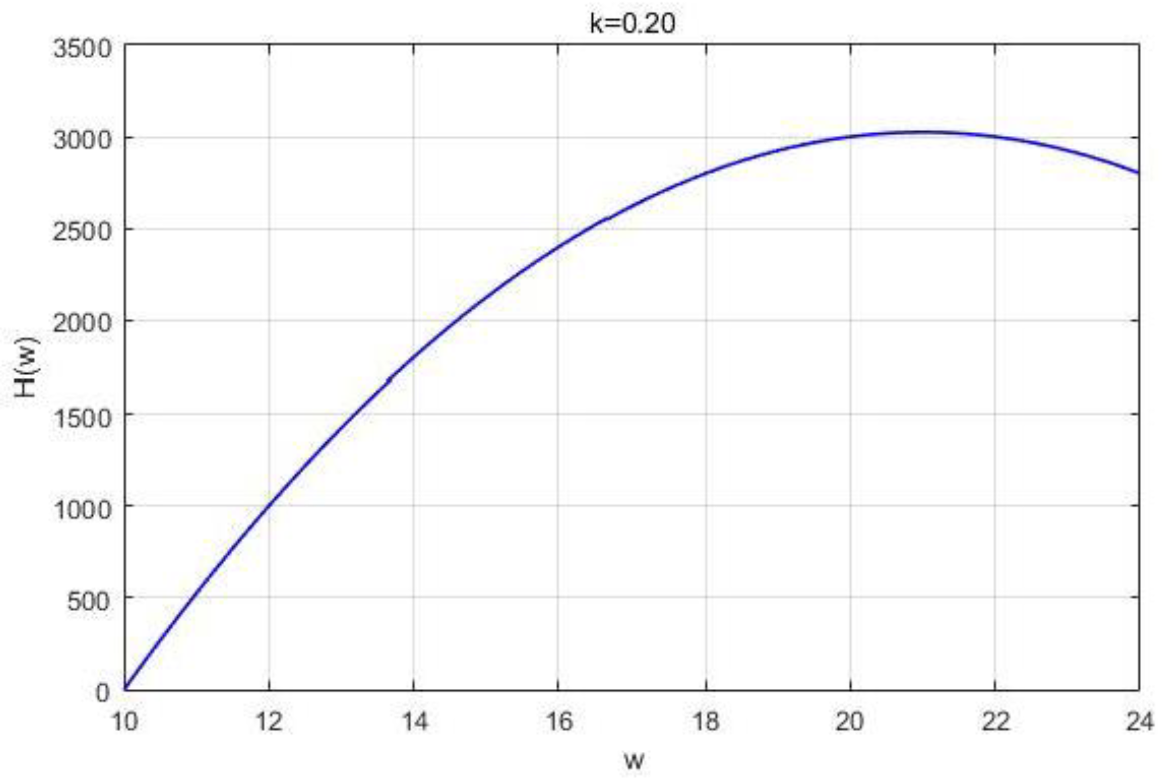
Firstly, in the range of φ < 1 6 , taking φ = 0.1 as an exemplar can indicate a certain regular variation. As shown in Figure 2, the supplier believes that the retailer will choose the retail price r c , when the wholesale price and the optimal retail price will remain constant within a smaller range of
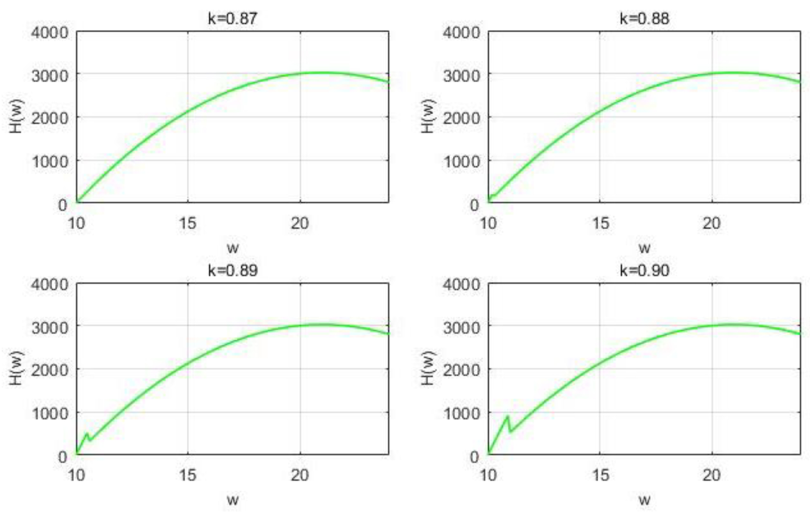
 κ . In Figure 3, there is a bound of κ between 0.87 and 0.88, which causes the supplier’s payoff function to change from a single peak to a double peak as the retailer’s confidence level declines.
Where the left peak in Figure 3 indicates that the supplier believes that this range of the retailer will lead them to choose the retail price r κ , the right peak remains constant. As κ rises, the left peak climbs, and the supplier’s optimal wholesale price stays the same up until it equals the right peak, taking the right peak point—a range where the retailer’s level of confidence has no bearing on the supplier’s decision. In 
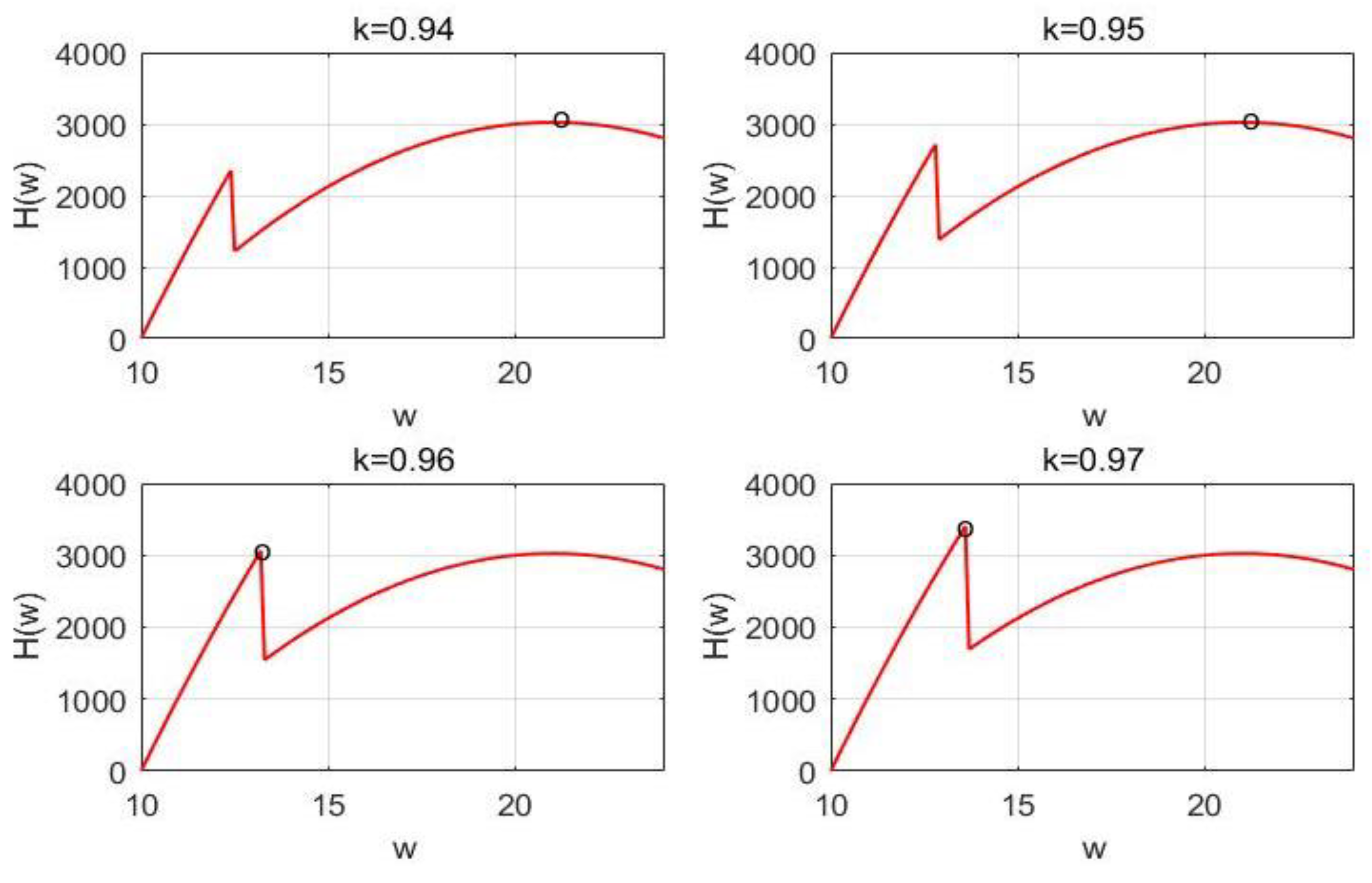
Figure 4, as the retailer’s confidence level decreases, the black circle indicates the maximum value of the function. Additionally, κ exists between 0.95 and 0.96 with bimodal equality, indicating that the supplier’s wholesale price decision will produce a sudden drop when the retailer’s confidence level decreases. As κ 
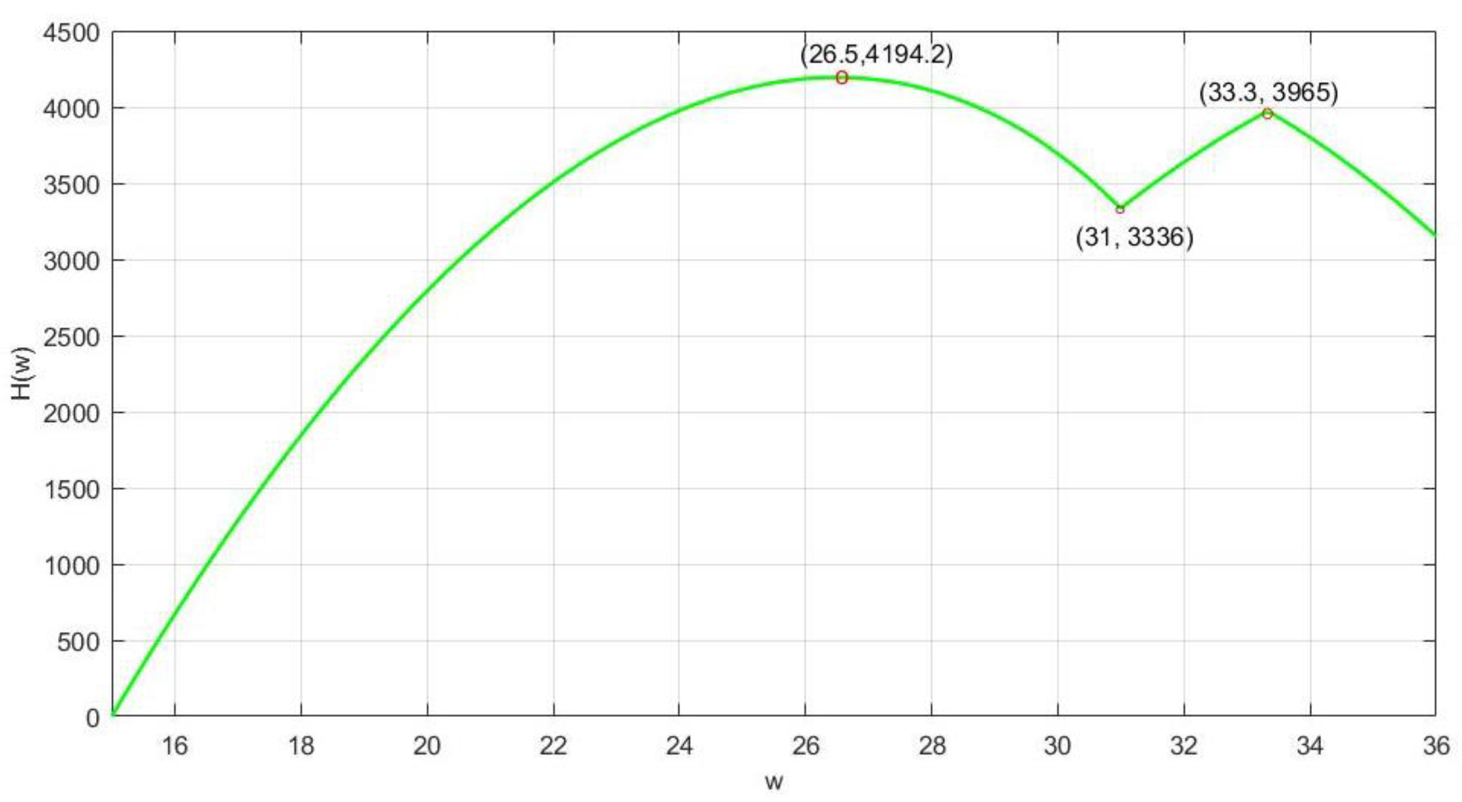
continues to increase, as shown in Figure 5, the range of retailer’s choice of r c gradually decreases and is occupied by r κ . When κ exceeds the threshold value of 1.1679, the supplier only considers the situation in which retailers accept r κ . At this point, both the wholesale price and the optimum retail price show a trend of first increasing and then decreasing, though the variations in both the wholesale and retail prices are very subtle. After the retailer’s confidence level falls to a certain bound, the supplier’s pricing decision roughly exhibits a monotonically increasing situation, converging to the highest wholesale price 24.
After that, we discuss the situation in the φ 1 6 , 5 16 . The overall change is more similar to the trend at φ = 0.1 , and the trend also changes from single-peak to double-peak and then to single-peak again. When φ = 0.3 the bimodal peaks already appear at smaller values of κ . The maximum payoff of the supplier increases as κ increases, with the change in κ between 0.2 and 0.3 appearing as the left peak enclosing the right peak. This trend indicates that for the supplier, the lack of confidence is the more favorable situation in the case of the degree of optimism of the retailer and the existence of opportunities to enable the supplier to reach a higher payoff.
Finally, we discuss the case when φ > 5 16 , when we can guarantee φ > φ 2 and satisfy the Theorem 3(iii). When φ = 0.4 and κ is small, the right peak in the double peak has been almost covered by the left, and the process of changing from a single peak to a double peak disappears. As the κ value increases currently, the image changes to a single-peak at a faster rate. When the φ value increases, it is almost a complete S-peak state.
When the φ value reaches a higher range, after the retailer optimism decreases significantly, the supplier believes that the retailer’s decision to choose the retail price is only r κ . When φ = 2 , the supplier’s payoff image that the image of the function (12), the change of the image is very insignificant; only when there is a large change in κ will it cause a subtle increase in the optimal wholesale price; as κ increases to higher range, the optimal wholesale price will be infinitely close to the upper limit of 24. The trend illustrates that when the value of φ is small, the change floats more and produces larger fluctuations according to the change in κ . As the value of φ increases, the payoff function of the supplier is gradually decreased by κ , and the trend becomes smaller and smaller. It indicates that when the retailer’s optimism is low, the supplier’s payoff is almost negligible by the retailer’s confidence level, and the supplier’s payoff fluctuates more only when the retailer is more optimistic.
The influence of the retailer’s optimism and self-confidence level on the decision can be obtained as follows:
(1) When the level of optimism and confidence of the retailer are both high, the pricing decision of the supplier and retailer do not produce fluctuations and are relatively stable. The best wholesale price will produce a trend from high to low as the retailer’s degree of confidence gradually declines while it is high.
(2) When the retailer’s optimism is determined, the lower the confidence level, the higher the supplier’s payoff.
The image comparison shows that it is more beneficial for the supplier to partner with a retailer who has a higher level of optimism and a lower level of confidence to expect payoff growth.

6. Comparison

6.1. Comparison with Classical Expectation Model

To compare and analyze whether supply chain coordination is possible under specific circumstances with decentralized decision-making by suppliers and retailers under positive focus decision-making, numerical experiments are substituted into the classical expectation value model in this section. According to the parameter settings in Section 5.1, the results of the classical model under considering only the expected payoff are shown in Table 8.
It is because the wholesale price is an endogenous variable that only the overall optimal retail price, as well as the payoff, are available in the results of the focus decision in Table 8. To present more clearly the coordination of the supply chain, the representative φ and κ are taken in combination with the data in the table and according to the range of the three φ values analyzed for the supplier’s payoff function to show the change curves of the expected payoff of the whole channel.
Figure 6 shows the change of the expected payoff image for each decision subject when φ = 0.1 , κ = 0.5 . The supplier will choose the wholesale price, 21. However, it can be seen in Figure 6 that the wholesale price cannot coordinate with the channel at this time. According to the influence of optimism degree and confidence level on decision-making analyzed in Section 5.1, with constant optimism of the retailer ( φ = 0.1 ) and increasing the value of κ , Figure 7 shows that the supply chain is close to coordination at φ = 0.1 , κ = 10 . At this point, the payoff of the whole channel corresponding to the point of the maximum payoff value of the supplier is infinitely close to the result under coordination. The image indicates that the supplier payoff and the channel payoff are close to overlap, while the retailer payoff is close to 0. It shows that when the retailer’s confidence level decreases infinitely, the channel payoff increases while leading to the loss of the retailer payoff.
On the other hand, the level of optimism of the retailer is adjusted. Increasing the value of φ with a constant level of retailer confidence, in contrast to Figure 7, which is nearly coordinated, Figure 8 depicts the payoff curve for the parameter configuration of φ = 0.4 , κ = 10 . The parameter settings in Figure 8 cannot coordinate the supply chain, but the existence of a certain range of wholesale prices makes the channel payoff infinitely close to the maximum value. This indicates that under certain circumstances, the wholesale price may change if the supplier can predict the form of the payoff distribution curve or if the supplier’s decision is not based exclusively on expected payoff maximization. The premise of this theory is to ensure that the overall payoff increase compensates for the supplier’s loss.

6.2. Comparison with Fairness Concern

Referring to the literature that first introduced fairness concern into the supply chain, the decision results are obtained by setting the retailer’s sensitive parameters α and β for advantageous inequality and disadvantageous inequality [42].
Table 9 shows that the fairness concern with α = 0.5 , β = 0.5 or α = 0.7 , β = 0.6 is able to coordinate the supply chain, in line with the results of Cui et al. [42]. In the fairness concern model, the supplier sets a wholesale price that aligns the incentives of all channel members with the interests of the entire channel so that the double-marginalization problem does not occur. When both advantageous inequality and disadvantageous inequality are high, the retailer with fairness concern will accomplish coordination in line with the findings of our outcomes. Additionally, it is further shown in conjunction with FTC that fixed wholesale price contracts can coordinate the supply chain as long as the retailer has certain fairness concern preference. There are good reasons for suppliers to choose this simpler and more feasible pricing mechanism.

6.3. Discussion on the Results

Combining the values of the classical expectation model in Figure 7 comparing Table 2 and Table 8, we find that channel coordination is likely to be achieved when the φ is small. As κ increases, the retail price of the final decision will keep approaching the optimal retail price under the classical model; that is, the wholesale price contract is likely to achieve channel coordination when the retailer is relatively optimistic and has a low level of confidence.
This finding further solidifies the importance of the retailer’s optimism and confidence levels for supply chain coordination under the FTC. Decision makers need to ensure cooperation and mutual benefits between supplier and retailer if they want to coordinate and achieve optimal channel payoffs. If channel coordination is premised on sacrificing the payoffs of one of the channel members, cooperation between the two decision makers is difficult to sustain in the long run, so this paper provides a theoretical basis for establishing further cooperation between supplier and retailer. To achieve channel coordination, the supplier can provide a certain allowance to the retailer to ensure that the retailer is not making zero payoffs, or a cooperation contract can be established between the supplier and the retailer to redistribute channel payoffs.
We introduce personality characteristics into the supply chain for modeling, and the result shows the impact of personality characteristics on supply chain coordination, leading to certain management insights on cooperation among decision makers as follows: The dominant supplier has the right to preferentially choose retailers. The above supplier can do this by recognizing the personality characteristic of the retailer through tests and by choosing retailers who are more optimistic and less confident. The retailer, as a follower, can modify his or her own optimism and self-confidence levels to promote supply chain coordination, improve the results of the classical expectation value model, and solve the double marginalization effect. In short, in any partnership, it is important to effectively consider the personality traits of the partner. Additionally, FTC can consider the influence of different personality characteristics in the decision-making process of decision makers, making the partnership in the supply chain more transparent and achieving profitable both sides.

7. Conclusions

The classical expectation value model using wholesale price contracts cannot coordinate the supply chain if the decision maker is fully rational, considering only the expected payoff. In this paper, the model considers the behavioral model under e-commerce and introduces the positive focus decision model to the retailer to study the coordination of the e-commerce supply chain under a wholesale price contract. The retailer’s decision is divided into two processes: the first process is to decide on the positive focus of potential demand in the product market of concern, and the second process is to select the retail price focus of concern among the positive demand focuses and determine the optimal retail price. The analysis shows that the wholesale price contract in the context of e-commerce may achieve channel coordination in the case of a more optimistic and low level of confidence of the retailer. Additionally, in many conditions, the realized payoffs are already better than the results of the classical expectation value model. At the same time, if the supplier is imperfectly rational, the conditions for coordinating the channel may become somewhat more lenient. Additionally, the supplier’s decisions may change depending on the degree of the retailer’s focus preference; that is, a retailer with a positive focus preference, different levels of optimism, and confidence can have a significant impact on channel coordination. With the supplier as the dominant player, it is a matter for further discussion in the supply chain to fully understand the personality traits and preferences of the retailer and how to make decisions that are more conducive to channel coordination without losing their interests.
The results of the model under focus preference corroborate that the positive focus preference of the study channel member is beneficial for coordinating the channel. The focus theory of choice contains two different evaluation systems. In the negative evaluation system, it is possible that an event that yields relatively lower returns with higher probability has higher salience for the decision maker, and if the retailer’s personality profile is biased toward the negative evaluation system, the conditions under the final channel coordination may be opposite to the results under the positive evaluation system. Additionally, in many cases, both evaluation systems may be present in the personality profile of the decision maker, and the retailer’s decision range may be somewhat broader and the conditions under channel coordination somewhat more lenient.
In business management, competition among retailers can be intense in the face of a complex e-commerce environment. The dominant supplier needs to comprehensively assess the retailer’s sales level, personality characteristics, and other factors. This paper shows that to promote supply chain coordination and improve overall channel performance, the supplier should choose retailers with a higher degree of positivity and a lower level of self-confidence to cooperate. The downstream retailers in the follower position, facing the competitive situation, need to improve their sales ability while reasonably adjusting their personality preference in the direction required by the supplier to improve the efficiency of cooperation. At the same time, there are various sales models in e-commerce, and retailers can improve the advantage of strategic market leadership to a certain extent through the reservation system, and they need to effectively protect the benefits of the consumers.
There is space for further expansion of the research. First, the model in this paper only assumes the existence of positive focus preference of the retailer, the supplier is assumed to be completely rational, and the subsequent research can study only the existence of focus preference of the supplier or both. Second, this paper does not have other costs, such as inventory costs; if the product can be sold by the retailer under a certain sales model, such as the reservation system, and can avoid a lot of cost output, many risk costs will be transferred to the consumer. However, if consumers are not satisfied with the product or the reservation time is too long, the return rate at a later stage will lead to higher maintenance costs, and the article will be further extended if the after-sale costs can be considered subsequently. Finally, the potential demand considered in this paper is linear and not general, and the potential demand of the market can be considered non-linear subsequently.

Author Contributions

Conceptualization, X.Z. and Y.S.; methodology, X.Z.; software, Y.S.; validation, X.Z., G.L. and W.X.; formal analysis, X.Z.; investigation, Y.S.; resources, W.X.; data curation, G.L.; writing—original draft preparation, Y.S.; writing—review and editing, X.Z.; visualization, G.L.; supervision, W.X.; project administration, G.L.; funding acquisition, W.X. All authors have read and agreed to the published version of the manuscript.

Funding

This research was funded by the National Natural Science Foundation of China, grant number Nos. 11901380, 12071280.

Institutional Review Board Statement

Not applicable.

Informed Consent Statement

Not applicable.

Data Availability Statement

Not applicable.

Conflicts of Interest

The authors declare no conflict of interest.

Appendix A

Proof of the Lemma 1.
π x is calculated according to the quadratic function of the normal distribution, and the optimization problem (4) is set up as a problem to solve the optimal solution of f x . First, because of r w , h > m , b w 2 l h < h , we can obtain x φ m , so Equation (6) holds. According to the range of x , we can obtain the size relationships as follows: if φ > 2 b r w h m a h b w 2   a n d   r < w + a φ h b w 2 2 b h m , satisfying x φ < h , the active focus of demand takes x φ at this point; if φ 2 b r w h m a h b w 2   a n d   r w + a φ h b w 2 2 b h m , satisfying x φ h , the active focus of demand takes h . Combining the range of values of retail price r , Lemma 1 is proved. □
Proof of the Lemma 2.
x P r , w = x φ is monotonically increasing with respect to r when r w , r 0 ; when r [ r 0 , l / b ] and x P ( r , w ) = h all the time. Since π · is monotonically increasing on the interval [ l , m ] and monotonically decreasing on the interval [ m , h ] , and x P r , w [ m , h ] , π · is monotonically decreasing about x P r , w . Therefore, according to the principle of composite functions, we know that π ( x P r , w ) is continuously monotonically decreasing about r on the interval [ w , r 0 ] and constant 1 a on the interval [ r 0 , l b ] . □
Proof of the Lemma 3.
For model (5), for the sake of simplicity, let g r = κ π ( x P r , w ) + u ( r , w , x P r , w ) . Substituting the positive demand focus x P of the first step into this function, g r can be expressed as g r = κ [ 1 a ( m x P r , w ) 2 ( h m ) 2 ] + 4 b r w ( x P r , w b r ) h b w 2 . The proving procedure consists of two steps.
  • Step 1: Solve the optimal solution of the function g r by interval.
When on the interval [ w , r 0 ] , x P ( r , w ) = x φ ,
g 1 ( r ) = 4 b 2 h b w 2 h m 2 2 φ κ φ 2 a h b w 2 1 r w 2 + 4 b m b w h b w 2 r w + κ .
The function g 1 ( r ) denotes the retailer’s optimization function on the interval [ w , r 0 ] , which is a quadratic function on r with symmetry axis r κ = w + a φ 2 h b w 2 ( m b w ) 2 b h m 2 ( κ 2 φ ) + 2 a b φ 2 h b w 2 and its quadratic term coefficient A = 4 b 2 h b w 2 h m 2 2 φ κ φ 2 a h b w 2 1 . When κ < 2 φ a φ 2 h b w 2 h m 2 , i.e., when A > 0 , it is easy to prove that r κ < w , when the optimal retail price is r 1 * = r 0 ; when κ 2 φ a φ 2 h b w 2 h m 2 , i.e., when A 0 , it is easy to prove that r κ w . In this case, the position of the symmetry axis is classified on the interval [ w , r 0 ] , and the optimal retail price under this condition is obtained as r 1 * = m i n { r 0 , r κ } .
According to the two classifications of A , the optimal retail price on the interval [ w , r 0 ] is
r 1 * = r 0 ,         if A > 0 , m i n { r 0 , r κ } , if A 0 .
when on the interval [ r 0 , l b ] , x P r , w = h , g 2 ( r ) = κ ( 1 a ) + 4 b r w ( h b r ) h b w 2 .
The function g 2 ( r ) is a quadratic function with a downward opening, and its axis of symmetry is r c = h + b w 2 b , according to the condition r c l b . According to the position of the axis of symmetry, r c can obtain the optimal retail price in the range of [ r 0 , l b ] as
r 2 * = m a x { r c , r 0 } .
  • Step 2: Solve for the global optimal retail price r P w and compare the magnitude of g 1 ( r 1 * ) and g 2 ( r 2 * ) .
When A > 0   o r   A 0   a n d   r 0 r κ , g 1 r 1 * = g 1 r 0 holds on w , r 0 ; g 2 r 0 g 2 r 2 * holds on the interval [ r 0 , l / b ] . The function g r is continuous with respect to r and satisfies the equation g 1 ( r 0 ) = g 2 ( r 0 ) , which leads to the inequality relation g 1 ( r 1 * ) = g 1 ( r 0 ) = g 2 ( r 0 ) g 2 ( r 2 * ) . The optimal retail price at this point is r P w = r 2 * = m a x { r c , r 0 } .
When A 0 , r 0 > r κ and r 0 = l / b , g 1 ( r 1 * ) = g 1 ( r κ ) > g 2 ( r 2 * ) is satisfied by taking r P w = r 1 * = r κ .
When A 0 , r 0 > r κ and r 0 = r φ , in the case r 2 * = r φ , g 1 ( r 1 * ) = g 1 ( r κ ) holds on the interval [ w , r 0 ] . Satisfying the relation g 1 ( r κ ) g 1 ( r 0 ) = g 2 ( r 2 * ) , we can obtain the optimal retail price at this time as r P w = r κ .
When A 0 , r 0 > r κ and r 0 = r φ , in the case r 2 * = r c , the function g r is continuous with respect to r and satisfies the inequality relation g 1 ( r κ ) g 1 ( r 0 ) = g 2 ( r 0 ) g 2 ( r c ) . Where the maximum values on the intervals [ w , r φ ] and [ r 0 , l / b ] , respectively, are
g 1 ( r κ ) = a φ 2 ( m b w ) 2 h m 2 ( κ 2 φ ) + a φ 2 h b w 2 + κ ,
g 2 ( r c ) = κ ( 1 a ) + 1 .
Taking the verification approach of judging the positive and negative of the difference between the two values, comparing the magnitude between g 1 ( r κ ) and g 2 ( r c ) such that G κ = g 1 r κ g 2 r c , we obtain
G κ = a φ 2 m b w 2 h m 2 κ 2 φ + a φ 2 h b w 2 + a κ 1 .
The first- and second-order derivatives of G κ are obtained as
G κ = a φ 2 m b w 2 h m 2 h m 2 κ 2 φ + a φ 2 h b w 2 2 + a ,
G κ = 2 a φ 2 m b w 2 h m 4 h m 2 κ 2 φ + a φ 2 h b w 2 h m 2 κ 2 φ + a φ 2 h b w 2 4 .
Because of A 0 κ κ 0 , where κ 0 = 2 φ a φ 2 h b w 2 h m 2 , we can prove that G κ 0 , while G κ is monotonically increasing. Letting G κ = 0 yields the zero of the first-order derivative G κ as κ 1 = 2 φ a φ 2 h b w 2 h m 2 + φ ( m b w ) h m . According to the preconditioner r φ > r κ of the fourth case, κ > κ 1 can be inferred, so G κ is monotonically increasing in the range of κ > κ 1 . The existence of the zero point of G κ for κ > κ 1 is further determined by making G κ = 0 have
a h m 2 κ 2 1 + 2 a φ h m 2 a 2 φ 2 h b w 2 κ + a φ 2 m b w 2 a φ 2 h b w 2 + 2 φ h m 2 = 0 .
The left and right roots of Equation (A1) are
κ 3 = κ 0 2 + 1 2 a + 1 2 a κ 0 2 2 φ 2 m b w 2 h m 2 ,
κ 4 = κ 0 2 + 1 2 a 1 2 a κ 0 2 2 φ 2 m b w 2 h m 2 .
Comparing the magnitude of the right root κ 3 with the zero κ 1 of the first-order derivative G κ , the difference can be obtained as follows:
κ 3 κ 1 = κ 0 2 + 1 2 a + 1 2 a κ 0 2 2 φ 2 m b w 2 h m 2 κ 0 + φ m b w h m = 1 2 a κ 0 2 φ m b w h m + 1 2 a κ 0 2 2 φ 2 m b w 2 h m 2 .
According to the inequality relation a φ h b w h m 2 2 a φ h b w h m + 1 0 , we can launch the relation of 1 2 a κ 0 2 φ m b w h m , which satisfies the size relationship κ 3 κ 1 . Similarly, it can be proved that κ 4 κ 1 . Based on the above comparison, it is shown that κ 1 ranges between the two zeros of G κ , which eventually leads to the following classification:
g 1 r κ g 2 r c < 0 , if κ 1 < κ < κ 3 , g 1 r κ g 2 r c 0 , if κ κ 3 .
Under the conditions that φ h m a ( h b w ) , κ > κ 1 are satisfied, the optimal retail price is chosen as
r P w = r c , if κ 1 < κ < κ 3 , r κ , if κ κ 3 .
The categorical proofs in the four cases eventually sum up to the form of Theorem 3, which is proved. □

References

  1. Cvsa, V.; Gilbert, S.M. Strategic commitment versus postponement in a two-tier supply chain. Eur. J. Oper. Res. 2002, 141, 526–543. [Google Scholar] [CrossRef]
  2. Spengler, J.J. Vertical integration and antitrust policy. J. Political Econ. 1950, 58, 347–352. [Google Scholar] [CrossRef]
  3. Arshinder; Kanda, A.; Deshmukh, S.G. Supply chain coordination: Perspectives, empirical studies and research directions. Int. J. Prod. Econ. 2008, 115, 316–335. [Google Scholar] [CrossRef]
  4. Ballou, R.H.; Gilbert, S.M.; Mukherjee, A. New managerial challenges from supply chain opportunities. Ind. Mark. Manag. 2000, 29, 7–18. [Google Scholar] [CrossRef]
  5. Lee, H.L.; Rosenblatt, M.J. A Generalized Quantity Discount Pricing Model to Increase Supplier’s Profits. Manag. Sci. 1986, 32, 1177–1185. [Google Scholar] [CrossRef]
  6. Deng, X.; Xie, J.; Xiong, H. Manufacturer–retailer contracting with asymmetric information on retailer’s degree of loss aversion. Int. J. Prod. Econ. 2013, 142, 372–380. [Google Scholar] [CrossRef]
  7. Kirshner, S.N.; Shao, L. Internal and external reference effects in a two-tier supply chain. Eur. J. Oper. Res. 2018, 267, 944–957. [Google Scholar] [CrossRef]
  8. Wang, C.X.; Webster, S. Channel Coordination for a Supply Chain with a Risk-Neutral Manufacturer and a Loss-Averse Retailer. Decis. Sci. 2007, 38, 361–389. [Google Scholar] [CrossRef]
  9. Vipin, B.; Amit, R.K. Wholesale price versus buyback: A comparison of contracts in a supply chain with a behavioral retailer. Comput. Ind. Eng. 2021, 162, 107689–107705. [Google Scholar] [CrossRef]
  10. Ren, Z.J.; Cohen, M.A.; Ho, T.H.; Terwiesch, C. Information Sharing in a Long-Term Supply Chain Relationship: The Role of Customer Review Strategy. Oper. Res. 2010, 58, 81–93. [Google Scholar] [CrossRef] [Green Version]
  11. Stewart, N.; Hermens, F.; Matthews, W.J. Eye Movements in Risky Choice. J. Behav. Decis. Mak. 2016, 29, 116–136. [Google Scholar] [CrossRef] [Green Version]
  12. Schweitzer, M.E.; Cachon, G.P. Decision Bias in the Newsvendor Problem with a Known Demand Distribution: Experimental Evidence. Manag. Sci. 2000, 46, 404–420. [Google Scholar] [CrossRef] [Green Version]
  13. Bachar, R.K.; Bhuniya, S.; Ghosh, S.K.; Sarkar, B. Controllable Energy Consumption in a Sustainable Smart Manufacturing Model Considering Superior Service, Flexible Demand, and Partial Outsourcing. Mathematics 2022, 10, 4517. [Google Scholar] [CrossRef]
  14. Gao, Y.T.; Johnson, N.; Shen, B.; Tan, Y.L. Benefits of sourcing alternative inputs of manufacturers for suppliers. Prod. Oper. Manag. 2023. [Google Scholar] [CrossRef]
  15. Hota, S.K.; Ghosh, S.K.; Sarkar, B. A solution to the transportation hazard problem in a supply chain with an unreliable manufacturer. AIMS Environ. Sci. 2022, 9, 354–380. [Google Scholar] [CrossRef]
  16. Sarkar, B.; Takeyeva, D.; Guchhait, R.; Sarkar, M. Optimized radio-frequency identification system for different warehouse shapes. Knowl.-Based Syst. 2022, 258, 109811. [Google Scholar] [CrossRef]
  17. Bendoly, E.; Boyer, K.; Craig, N.; Paul, S. Pulled in opposite directions: A joint consideration of supply and demand uncertainty in supply chain decision-making. J. Bus. Logist. 2022, 43, 448–471. [Google Scholar] [CrossRef]
  18. Lariviere, M.A.; Porteus, E.L. Selling to the Newsvendor: An Analysis of Price-Only Contracts. Manuf. Serv. Oper. Manag. 2001, 3, 293–305. [Google Scholar] [CrossRef]
  19. Holmstrom, B.; Milgrom, P. Aggregation and Linearity in the Provision of Intertemporal Incentives. Econometrica 1987, 55, 303–328. [Google Scholar] [CrossRef] [Green Version]
  20. Cachon, G.P.; Lariviere, M.A. Supply Chain Coordination with Revenue-Sharing Contracts: Strengths and Limitations. Manag. Sci. 2005, 51, 30–44. [Google Scholar] [CrossRef] [Green Version]
  21. Pasternack, B.A. Optimal Pricing and Return Policies for Perishable Commodities. Mark. Sci. 1985, 4, 166–176. [Google Scholar] [CrossRef]
  22. Katok, E.; Wu, D.Y. Contracting in Supply Chains: A Laboratory Investigation. Manag. Sci. 2009, 55, 1953–1968. [Google Scholar] [CrossRef] [Green Version]
  23. Zhang, Y.; Donohue, K.; Cui, T.H. Contract Preferences and Performance for the Loss-Averse Supplier: Buyback vs. Revenue Sharing. Manag. Sci. 2016, 62, 1734–1754. [Google Scholar] [CrossRef]
  24. Li, M.W.; Shan, M.Y. Pricing and green promotion effort strategies in dual-channel green supply chain: Considering e-commerce platform financing and free-riding. J. Bus. Ind. Mark. 2023. [Google Scholar] [CrossRef]
  25. Wang, Y.Y.; Tan, Y.; Wang, J.C.; Lai, F.J. Uniform vs. retailer-specific pricing: How a supplier responds to the dominant retailers’ markup pricing strategy. J. Oper. Res. Soc. 2023. [Google Scholar] [CrossRef]
  26. Zhao, Z.Z.; Liu, Y.X.; Guo, L.; Bai, L.Q.; Wang, Z.G.; Wang, C.S. Distribution Locational Marginal Pricing Under Uncertainty Considering Coordination of Distribution and Wholesale Markets. IEEE Trans. Smart Grid 2023, 14, 1590–1606. [Google Scholar] [CrossRef]
  27. Bernstein, F.; Chen, F.; Federgruen, A. Coordinating Supply Chains with Simple Pricing Schemes: The Role of Vendor-Managed Inventories. Manag. Sci. 2006, 52, 1483–1492. [Google Scholar] [CrossRef] [Green Version]
  28. Qiu, R.; Yu, Y.; Sun, M. Supply chain coordination by contracts considering dynamic reference quality effect under the O2O environment. Comput. Ind. Eng. 2022, 163, 107802. [Google Scholar] [CrossRef]
  29. Shu, W.J.; Xiao, Z.D.; Cao, Y.Y. How the agency contract fails in hybrid mode: Agency fees and distribution sequences. Int. Trans. Oper. Res. 2023. [Google Scholar] [CrossRef]
  30. Becker-Peth, M.; Thonemann, U.W. Reference points in revenue sharing contracts—How to design optimal supply chain contracts. Eur. J. Oper. Res. 2016, 249, 1033–1049. [Google Scholar] [CrossRef]
  31. Von Neumann, J.; Morgenstern, O. Theory of Games and Economic Behavior: 60th Anniversary Commemorative Edition; Princeton University Press: Princeton, NJ, USA, 1953. [Google Scholar] [CrossRef]
  32. Allais, M. Le comportement de l’homme rationnel devant le risque: Critique des postulats et axiomes de l’école américaine. Econom. J. Econom. Soc. 1953, 21, 503–546. [Google Scholar] [CrossRef] [Green Version]
  33. Ellsberg, D. Risk, ambiguity, and the Savage axioms. Q. J. Econ. 1961, 75, 643–669. [Google Scholar] [CrossRef] [Green Version]
  34. Bolton, G.E.; Katok, E. Learning by Doing in the Newsvendor Problem: A Laboratory Investigation of the Role of Experience and Feedback. Manuf. Serv. Oper. Manag. 2008, 10, 519–538. [Google Scholar] [CrossRef] [Green Version]
  35. Corbett, C.J.; Van Wassenhove, L.N. The Natural Drift: What Happened to Operations Research? Oper. Res. 1993, 41, 625–640. [Google Scholar] [CrossRef] [Green Version]
  36. Meredith, J.R. Reconsidering the Philosophical Basis of OR/MS. Oper. Res. 2001, 49, 325–333. [Google Scholar] [CrossRef]
  37. Bostian, A.A.; Holt, C.A.; Smith, A.M. Newsvendor “Pull-to-Center” Effect: Adaptive Learning in a Laboratory Experiment. Manuf. Serv. Oper. Manag. 2008, 10, 590–608. [Google Scholar] [CrossRef] [Green Version]
  38. Hämäläinen, R.P.; Luoma, J.; Saarinen, E. On the importance of behavioral operational research: The case of understanding and communicating about dynamic systems. Eur. J. Oper. Res. 2013, 228, 623–634. [Google Scholar] [CrossRef]
  39. Fang, C.; Ma, X.; Zhang, J.; Zhu, X. Personality information sharing in supply chain systems for innovative products in the circular economy era. Int. J. Prod. Res. 2021, 59, 5992–6001. [Google Scholar] [CrossRef]
  40. Camerer, C.; Lovallo, D. Overconfidence and excess entry: An experimental approach. Am. Econ. Rev. 1999, 89, 306–318. [Google Scholar] [CrossRef] [Green Version]
  41. Fehr, E.; Schmidt, K.M. A theory of fairness, competition, and cooperation. Q. J. Econ. 1999, 114, 817–868. [Google Scholar] [CrossRef] [Green Version]
  42. Haitao Cui, T.; Raju, J.S.; Zhang, Z.J. Fairness and Channel Coordination. Manag. Sci. 2007, 53, 1303–1314. [Google Scholar] [CrossRef] [Green Version]
  43. Ho, T.-H.; Lim, N.; Cui, T.H. Reference dependence in multilocation newsvendor models: A structural analysis. Manag. Sci. 2010, 56, 1891–1910. [Google Scholar] [CrossRef]
  44. Tversky, A.; Kahneman, D. Judgment under Uncertainty: Heuristics and Biases: Biases in judgments reveal some heuristics of thinking under uncertainty. Science 1974, 185, 1124–1131. [Google Scholar] [CrossRef]
  45. Tversky, A.; Kahneman, D. Advances in prospect theory: Cumulative representation of uncertainty. J. Risk 1992, 5, 297–323. [Google Scholar] [CrossRef]
  46. Majeed, A.; Wang, Y.; Muniba; Islam, M.A. The Impact of Social Preferences on Supply Chain Performance: An Application of the Game Theory Model. Complexity 2023, 2023, 4911514. [Google Scholar] [CrossRef]
  47. Guo, P. Focus theory of choice and its application to resolving the St. Petersburg, Allais, and Ellsberg paradoxes and other anomalies. Eur. J. Oper. Res. 2019, 276, 1034–1043. [Google Scholar] [CrossRef]
  48. Guo, P.; Zhu, X. Focus Programming: A Fundamental Alternative for Stochastic Optimization Problems. SSRN Electron. J. 2019. Available online: https://ssrn.com/abstract=3334211 (accessed on 1 April 2023). [CrossRef]
  49. Zhu, X.; Guo, P. Approaches to four types of bilevel programming problems with nonconvex nonsmooth lower level programs and their applications to newsvendor problems. Math. Methods Oper. Res. 2017, 86, 255–275. [Google Scholar] [CrossRef]
  50. Guo, P. Dynamic focus programming: A new approach to sequential decision problems under uncertainty. Eur. J. Oper. Res. 2022, 303, 328–336. [Google Scholar] [CrossRef]
  51. Zhu, X.; Guo, P. Single-level reformulations of a specific non-smooth bilevel programming problem and their applications. Optim. Lett. 2020, 14, 1393–1406. [Google Scholar] [CrossRef]
  52. Zhu, X.; Li, K.W.; Guo, P. A bilevel optimization model for the newsvendor problem with the focus theory of choice. 4OR-A Q. J. Oper. Res. 2023. [Google Scholar] [CrossRef]
  53. Zhu, X.; Xie, L.; Lin, G.; Ma, X. Decision analysis of individual supplier in a vendor-managed inventory program with revenue-sharing contract. Int. J. Ind. Eng. Comput. 2022, 13, 405–420. [Google Scholar] [CrossRef]
  54. Zhu, X.; Hu, Z.; Lin, G.; Xu, W. Strategy Analysis for Retailer-Leading Supply Chain under Buyback Contract with Focus Theory of Choice. Mathematics 2023, 11, 664. [Google Scholar] [CrossRef]
  55. Li, M. Overconfident Distribution Channels. Prod. Oper. Manag. 2019, 28, 1347–1365. [Google Scholar] [CrossRef]
  56. Wu, X.; Niederhoff, J.A. Fairness in Selling to the Newsvendor. Prod. Oper. Manag. 2014, 23, 2002–2022. [Google Scholar] [CrossRef]
  57. Xiao, Q.; Chen, L.; Xie, M.; Wang, C. Optimal contract design in sustainable supply chain: Interactive impacts of fairness concern and overconfidence. J. Oper. Res. Soc. 2020, 72, 1505–1524. [Google Scholar] [CrossRef]
  58. Zhao, X.; Si, D.; Zhu, W.; Xie, J.; Shen, Z.J. Behaviors and Performance Improvement in a Vendor-Managed Inventory Program: An Experimental Study. Prod. Oper. Manag. 2019, 28, 1818–1836. [Google Scholar] [CrossRef]
  59. Zhu, X.; Guo, P. Bilevel programming approaches to production planning for multiple products with short life cycles. 4OR-A Q. J. Oper. Res. 2020, 18, 151–175. [Google Scholar] [CrossRef]
Figure 1. Reference model of the supplier’s payoff function.
Jtaer 18 00053 g001
Figure 2. Image change (1) of H ( w ) with φ = 0.1 .
Jtaer 18 00053 g002
Figure 3. Image changes (2) of H ( w ) with φ = 0.1.
Jtaer 18 00053 g003
Figure 4. Image changes (3) of H ( w ) with φ = 0.1.
Jtaer 18 00053 g004
Figure 5. Image changes (4) of H ( w ) with φ = 0.1.
Jtaer 18 00053 g005
Figure 6. Payoff image changes with φ = 0.1 , κ = 0.5 .
Jtaer 18 00053 g006
Figure 7. Payoff image changes with φ = 0.1 , κ = 10 .
Jtaer 18 00053 g007
Figure 8. Payoff image changes with φ = 0.4 , κ = 10 .
Jtaer 18 00053 g008
Table 1. Variable Definition.
NotationDefinition
r retail price/unit
w wholesale price/unit
x the market potential demand
b the sensitivity of product market demand concerning the retail price
c the supplier’s cost of production/unit
v s / v r / v the payoff function of the supplier/retailer/supply chain in the classical model
φ the retailer’s degree of optimism
κ the retailer’s level of confidence
u · the retailer’s satisfaction function
π · the relative likelihood function
l / h / m the minimum/maximum/average values of market potential demand
x P · the positive demand focus of the retailer concerns
r P · the optimal retail price of the retailer concerns
H · the payoff function of the supplier in the classical model
Table 2. Solutions of the proposed model with φ = 0.1 .
κ w p * r P w p * H w p * u w p * , x P ( r P w p * , w p * ) π x P ( r P w p * , w p * )
0.12130.5302510.2
0.52130.5302510.2
114.817.843650.40.8
223.323.88141.90.11
1023.123.28388.80.011
Table 3. Solutions of the proposed model with φ = 0.3 .
κ w p * r P w p * H w p * u w p * , x P ( r P w p * , w p * ) π x P ( r P w p * , w p * )
0.123.331.72881.610.2
0.522.229.63891.50.90.5
12428.55282.50.70.7
22428.56504.10.70.7
1023.624.37951.10.11
Table 4. Solutions of the proposed model with φ = 0.5 .
κ w p * r P w p * H w p * u w p * , x P ( r P w p * , w p * ) π x P ( r P w p * , w p * )
0.120.129.83122.60.80.8
0.521.529.73617.10.80.8
12329.542250.70.8
22428.652000.60.9
102425.67298.40.31
Table 5. Solutions of the proposed model with φ = 1 .
κ w p * r P w p * H w p * u w p * , x P ( r P w p * , w p * ) π x P ( r P w p * , w p * )
0.121.529.73648.10.71
0.521.929.73771.90.71
122.329.63925.50.71
22329.542250.71
102427.75815.40.51
Table 6. Solutions of the proposed model with φ = 2 .
κ w p * r P w p * H w p * u w p * , x P ( r P w p * , w p * ) π x P ( r P w p * , w p * )
0.122.229.639330.61
0.522.429.63963.60.61
122.529.64001.50.61
222.629.54076.80.61
1023.929.34640.90.61
Table 7. Solutions of the proposed model with φ = 10 .
κ w p * r P w p * H w p * u w p * , x P ( r P w p * , w p * ) π x P ( r P w p * , w p * )
0.122.929.541660.61
0.522.929.54167.60.61
122.929.54169.10.61
222.929.54172.10.61
1022.929.54195.70.61
Table 8. Results of the classical expectation model.
r V r w * V s V
Centralization23///8450
Decentralization29.52112.52342256337.5
Table 9. Results of the fairness concern model.
θ I n e q u a l i t y   P a r a m e t e r s w * r w * Supplier ProfitChannel Profit
θ = 1 α = 0.5 , β = 0.2 182640008000
θ = 1 α = 0.5 , β = 0.4 17.124.24190.18380.2
θ = 1 α = 0.5 , β = 0.5 16.52342258450
θ = 1 α = 0.6 , β = 0.4 17.124.24190.18380.2
θ = 1 α = 0.7 , β = 0.6 16.52342258450
Note: θ represents the retailer’s equitable payoff parameter. α and β represent the retailer’s disadvantageous and advantageous inequality parameters, respectively.
Disclaimer/Publisher’s Note: The statements, opinions and data contained in all publications are solely those of the individual author(s) and contributor(s) and not of MDPI and/or the editor(s). MDPI and/or the editor(s) disclaim responsibility for any injury to people or property resulting from any ideas, methods, instructions or products referred to in the content.

