Recent Advancements in Computational Drug Design Algorithms through Machine Learning and Optimization

Abstract

The goal of drug discovery is to uncover new molecules with specific chemical properties that can be used to cure diseases. With the accessibility of machine learning techniques, the approach used in this search has become a significant component in computer science in recent years. To meet the Precision Medicine Initiative’s goals and the additional obstacles that they have created, it is vital to develop strong, consistent, and repeatable computational approaches. Predictive models based on machine learning are becoming increasingly crucial in preclinical investigations. In discovering novel pharmaceuticals, this step substantially reduces expenses and research times. The human kinome contains various kinase enzymes that play vital roles through catalyzing protein phosphorylation. Interestingly, the dysregulation of kinases causes various human diseases, viz., cancer, cardiovascular disease, and several neuro-degenerative disorders. Thus, inhibitors of specific kinases can treat those diseases through blocking their activity as well as restoring normal cellular signaling. This review article discusses recent advancements in computational drug design algorithms through machine learning and deep learning and the computational drug design of kinase enzymes. Analyzing the current state-of-the-art in this sector will offer us a sense of where cheminformatics may evolve in the near future and the limitations and beneficial outcomes it has produced. The approaches utilized to model molecular data, the biological problems addressed, and the machine learning algorithms employed for drug discovery in recent years will be the emphasis of this review.

1. Introduction

Traditional drug discovery and development processes are widely recognized for taking a long time and costing a lot of money. The complete process of developing a new drug to come into the market takes an average of 10 to 15 years, and an estimated 58.8 billion dollars had been spent on new drug development as of 2015. For both the biotechnology and pharmaceutical industries, these figures represent a remarkable 10 percent growth over previous years. Out of millions of chemical compounds, only 1 percent will proceed to clinical testing. Only 5–10 compounds will typically be tested in the human body. Furthermore, a 1995–2007 study by the Tufts Center for the Study of Drug Development found that only 11.83 percent of drugs that advance to Phase I of clinical trials were ultimately brought to market. Additionally, from 2006 to 2015, only 9.6 percent of drugs undergoing clinical trials were successful. The exorbitantly high expenditure and failure rates of these traditional drug discovery processes have forced researchers to find an alternative method. Computer-aided drug discovery (CADD) algorithms are employed for the fast design of new drugs. CADD is a specialized branch that uses computational methods to model drug receptor interactions in order to evaluate if a given chemical will attach to a target and, if so, with what affinity [1]. This methodology has become the most extensively used method for reducing the number of potential medicinal compounds from a huge library by predicting the activity. For high-throughput screening, this method requires much less money and time while maintaining high lead-finding quality. Ligands can bind to receptors in various ways, including hydrophobic, electrostatic, and hydrogen-bonding interactions. CADD’s main goal is to screen, optimize, and analyze the compound’s activity against the target. It is a multi-disciplinary technique that is used by both academic institutions and commercial pharmaceutical businesses to improve efficacy while minimizing or eliminating negative effects. A large number of compounds are screened based on structure prediction, target identification, binding site prediction, protein–ligand interactions, etc. Then, the results are tallied with the ADMET properties. The ADMET (adsorption, distribution, metabolism, excretion, and toxicity) properties are screened to increase the success rate and decrease the time for drug discovery. In this article, we discuss the computational drug design of the human kinome. The kinome denotes the entire family of protein and lipid kinases, which are enzymes playing a vital role to regulate cell signaling pathways. By phosphorylating specific proteins, kinases can control cellular processes, viz., cell division, differentiation, and death [2]. The dysregulation of kinases promotes various human diseases, including cancer, cardiovascular disease, and neuro-degenerative disorders [3]. Hence, kinases have become a major target for drug discovery as well as development in the entire pharmaceutical industry.

2. Biological and Computational Terms

• Ligands: Molecules or ions that are coordinated with the central atom or ion in the coordination compound are called ligands.
• Molecular descriptors: Molecular descriptors are numerical representations of molecule attributes. Physical and chemical properties of the molecule are numerically represented by molecular descriptors [4].
• Molecular docking: Docking is a method of molecular modeling that predicts the preferred orientation of a ligand when it is bound in an active site of a molecule to form a stable complex [5].
• Molecular dynamics: Molecular dynamics (MD) is a computer simulation method for analyzing the physical movement of atoms and molecules. The atoms and molecules are allowed to interact for a fixed period of time, giving a dynamic view of the system. MD simulation is based on Newton’s second law or the equation of motion.

3. Importance of Computational Drug Discovery

Drug design, discovery, and development are time-consuming and tedious inter-disciplinary processes encompassing many different domains of study [6]. Traditional drug discovery and development are widely recognized for taking a long time and costing a lot of money, e.g., an average of 10 to 15 years to get to market and costing an estimated 58.8 billion dollars as of 2015 [7,8]. Among 10,000 chemical compounds, only 200–250 will proceed to clinical testing. Among these 200–250 compounds, 10 will be tested in animals rather than in the human body. Tufts Center for the Study of Drug Development conducted a study from 1995 to 2007, which stated that out of all drug molecules that proceed to Phase I of clinical trials, roughly 11.83 percent are approved for market. The high cost and failure rates of traditional drug discovery have forced researchers to execute a new path for drug discovery. CADD has provided a new way to accelerate the drug discovery process.

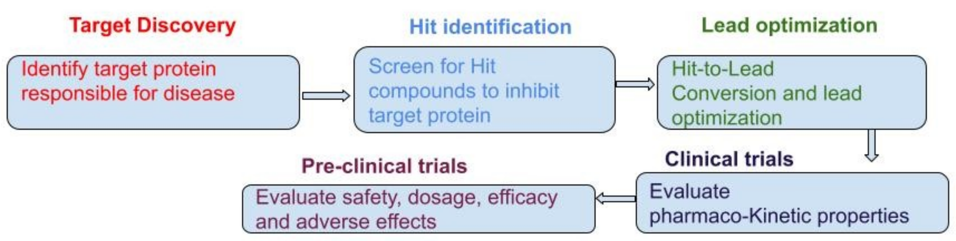
4. Process of Drug Discovery

Drug design is a lengthy and time-consuming process. It has several steps from target discovery to clinical trials. There are several computational methods that can be utilized in each computational step, starting from target discovery to clinical trials [9].

We have provided a flowchart (Figure 1) of all the computational techniques that help in different stages of drug discovery. Some impressive computational drug discovery and development approaches and platforms have been devised and built. Several approaches and platforms are discussed in this section, including target identification, docking-based virtual screening, conformation sampling, scoring functions, molecular similarity computation, virtual library design, and sequence-based drug design. These elements are intertwined, and improvements in one may help the others (Figure 2).

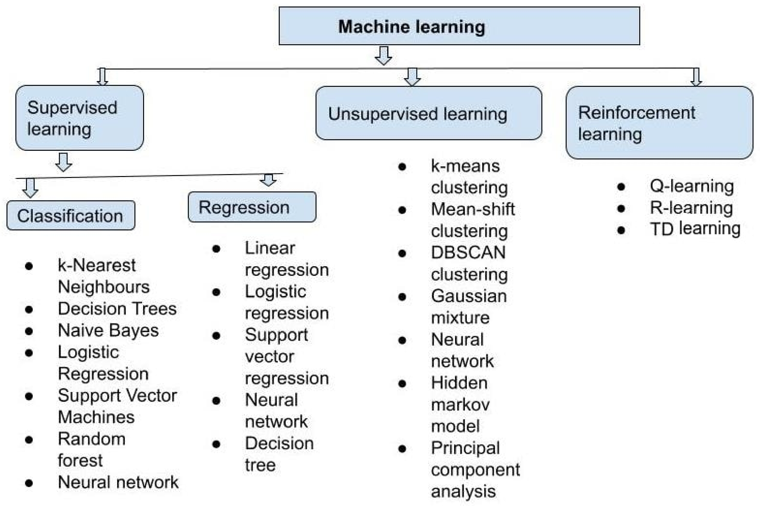
5. Machine Learning and Deep Learning Techniques Used for Drug Discovery

There are numerous molecular modeling and molecular docking techniques that researchers have been using for a long time. Recent advances in machine learning and deep learning techniques have significantly accelerated the drug design process. These techniques are widely used by both academia and industries. These machine learning algorithms are usually data-hungry and fortunately, there is no dearth of data in the world today. Lots of relevant chemical and biological datasets are publicly available now for machine and deep learning models. Machine learning models are being used in drug discovery for data mining, data analysis, predicting the chemical and physical properties of molecules, etc. We can divide machine learning techniques into three categories and in each category we have different types of algorithms. We have given a flowchart of different categories in Figure 3.

When we feed a dataset into a machine learning model, generally the dataset is divided into training and test sets. A training set is used in supervised learning to train models to produce the desired output. This training dataset has an input and an output and we approximate a function f(x) over training data points. We use a loss function ($L_{\epsilon }$) to assess the model’s correctness, and the parameters are modified using gradient descent until the error is suitably minimized.

$$p_{n+1}=p_n-\nabla L_{\epsilon }$$

$$\because n=\mathrm{number}\mathrm{of}\mathrm{steps},p=\mathrm{parameter}\mathrm{vector}$$

• We can divide supervised learning into two categories: (1) classification and (2) regression. A classification algorithm is used to classify test data and allocate it to certain groups. It recognizes certain entities in the dataset and makes educated guesses about how those entities should be labeled or defined. Linear classifiers, support vector machines (SVMs), decision trees, k-nearest neighbor, and random forest are some of the most common classification algorithms. To explore the relationship between dependent and independent variables, regression is used. It is widely used to produce predictions, such as for a company’s sales revenue. Popular regression algorithms include linear regression, logistical regression, and polynomial regression.

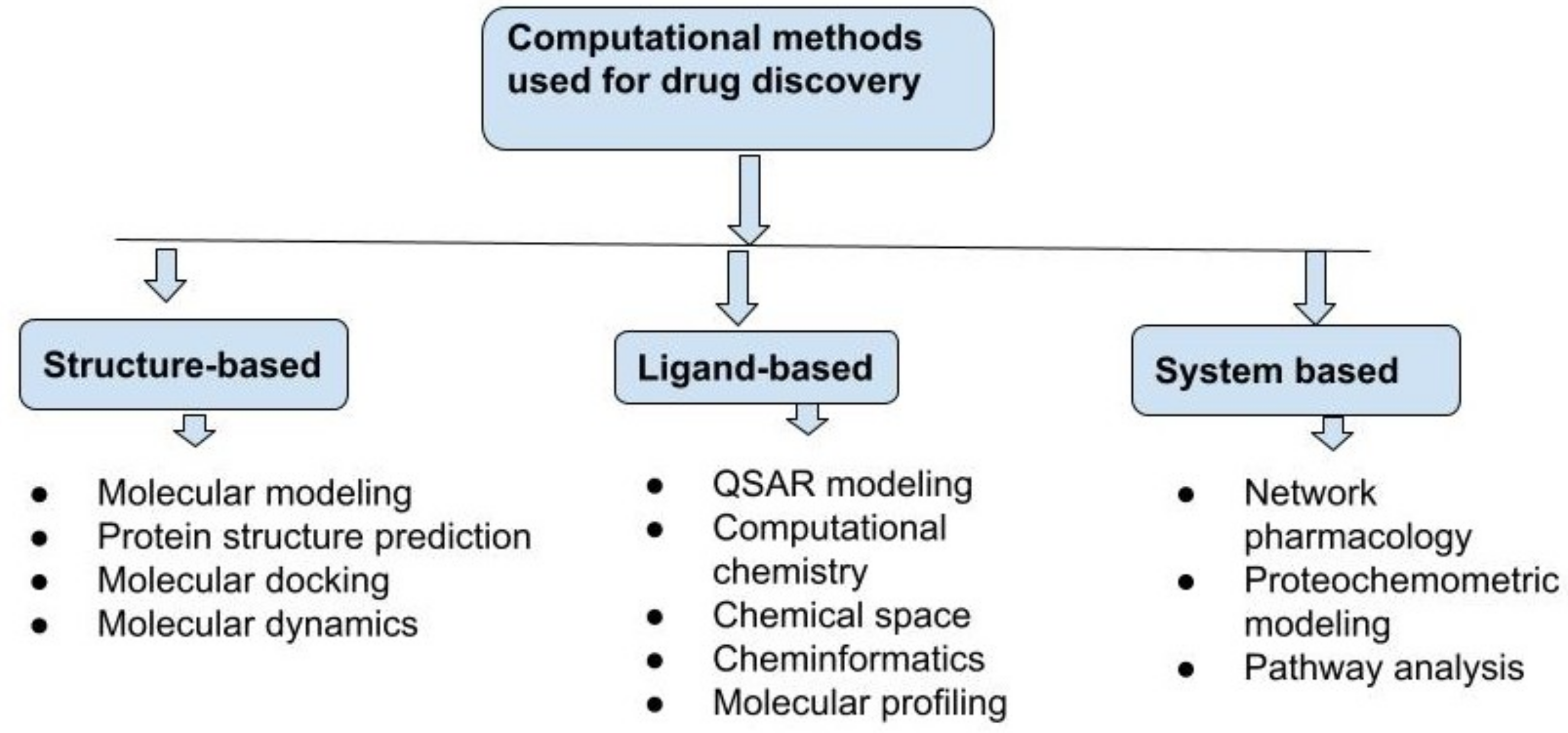
6. Different Approaches for Computational Drug Discovery

In this section, we will briefly describe some of the computational techniques that have been widely used in drug discovery.

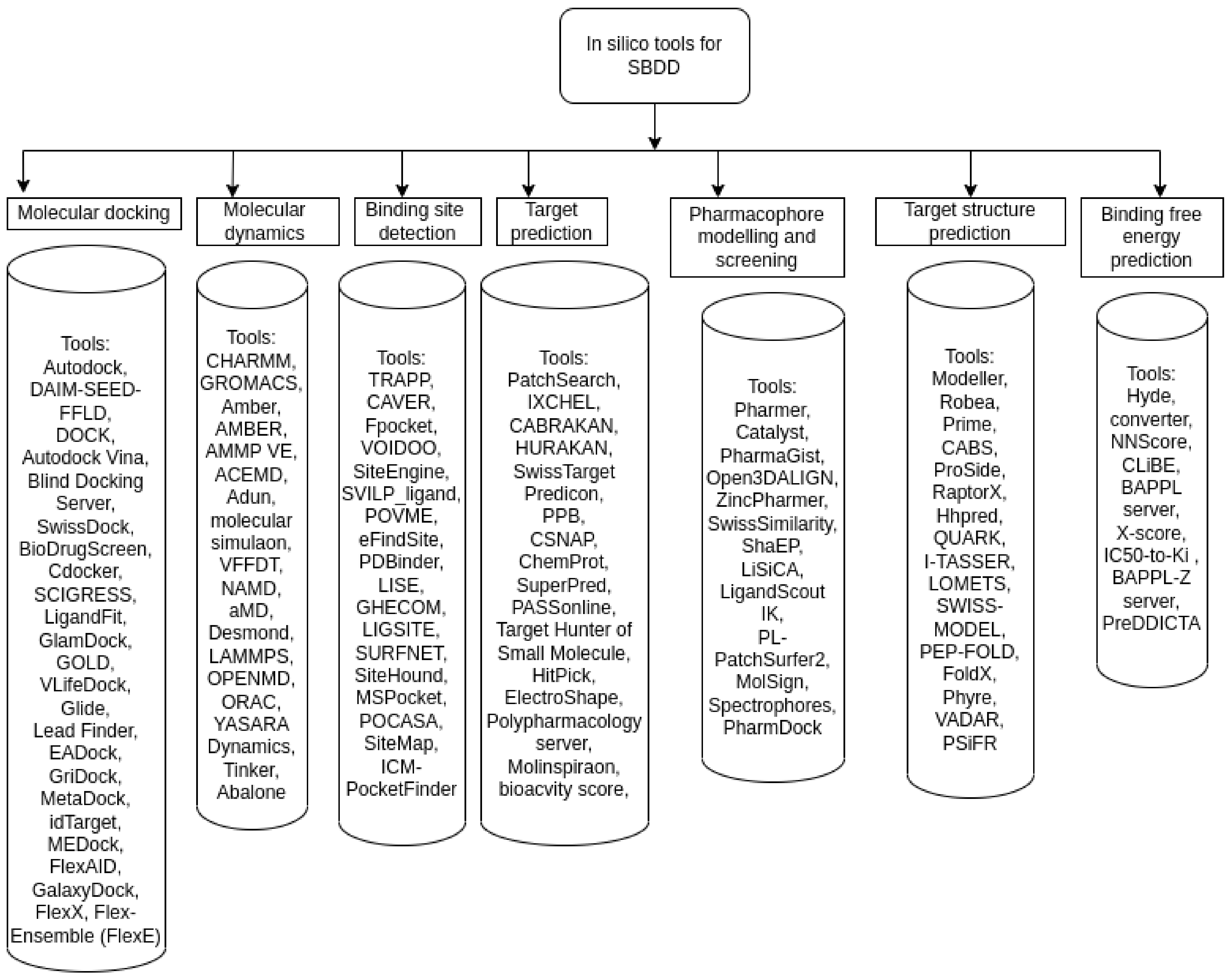
6.1. Structure-Based Drug Discovery

Drug design began approximately three decades ago with the utilization of the 3D structure information of proteins and DNA. Structure-based drug design is one of the oldest drug design techniques. Recent advancements in proteomics, genomics, and bioinformatics have given us the 3D structures of huge numbers of proteins. Recently, Deepmind has released AlphaFold, an AI system that can predict a protein 3D structure from its amino acid sequence [10]. AlphaFold has predicted the 3D structure of all the human proteins. The availability of a huge number of target protein 3D structures has significantly accelerated the processes in SBDD (Figure 4). Molecular docking and molecular dynamics are the two computational methods that were traditionally used for a long time in SBDD. Now, advancements in deep learning and cloud computing have given new directions to SBDD protocols (Figure 5). A huge amount of 3D structure data has forced us towards data-driven structure-based drug discovery. The Protein Data Bank (PDB) [11] is the world’s largest repository of bio-molecule structure data derived mostly from X-ray crystallography and nuclear magnetic resonance (NMR) techniques. The Protein Data Bank had 2058 structures deposited in 1998. Since then, the number of structures deposited has increased by 7.5 percent each year, totaling 188,923 in 2014. For years, the exploitation of this wealth of structural data has been the cornerstone of structure-based medication creation in academia and the pharmaceutical sector. Proteins are dynamic macro-molecules by nature. The first step of SBDD after identifying a target protein is finding the binding pocket of the target protein. The binding pocket is the cavity where a small molecule will be bound to obtain the desired result. Therefore, it is important to identify the binding site of the target protein. There are few computational methods that can find the binding sites of a molecule. These methods use the interaction energy and van der Waals (vdW) forces for binding site mapping. An energy-based technique for predicting binding sites is Q-SiteFinder [12]. The next phase is hit discovery, which is carried out by docking chemical libraries into the target protein’s binding cavity. Molecular docking is a technique that has been used for the virtual simulation of molecular interactions. Molecular docking has been widely used in SBDD. This method predicts the conformation and binding of ligands within a target active site with excellent precision [13,14]. Molecular docking gives binding energies and ranks the ligands in a dataset according to different scoring functions. As a result, studying a protein’s interaction with a small molecule, or simply identifying its binding site, requires more than a structural snapshot. Molecular dynamics (MD) simulations are the widely used methods to understand a protein’s behavior. MD is used to calculate the trajectory of conformations as a function of time using Newtonian mechanics and force fields such as Amber [15] or CHARMm [16]. There are some MD applications, such as free energy perturbation (FEP) methods [17], molecular mechanics/Poisson–Boltzmann surface area (MM/PBSA) [18], and linear interaction energy (LIE) [19], which have been used for free energy calculations to check the correlation of experimental and calculated binding affinities of small molecules to proteins. These methods can then be utilized to predict binding affinities in a computer simulation. Now, deep learning is trying to replace all the techniques that have been used for a long time in SBDD. Deep learning is used for protein–ligand binding site prediction [20], protein–ligand binding affinity prediction [21], etc. If the structure of a protein is not known for some reason, then we can use homology modeling. Homology modeling is used to build a protein model after identifying a structural template protein with a similar sequence, aligning their sequences, using aligned region coordinates, predicting missing atom coordinates of the target, model building, and refinement. MODELER [22] and SWISS-MODEL [23] are two widely used programs for homology.

6.2. Ligand-Based Drug Discovery

Ligand-based drug design is used when we do not have the necessary information about the 3D structure of a molecule. It relies on the knowledge that molecules bind to the biological target of interest. LBDD is based on the similar property principal, which states that similarly structured molecules have similar biochemical properties. LBDD uses different methods for describing the features of small molecules using computational algorithms. We use molecular descriptors to encode the structural and physicochemical properties of a molecule. These encoded properties are generally the weight, logP, volume, geometry, surface area, ring content, rotatable bond, interatomic distance, bond distance, atom types, planner and non-planner system, electronegativity, polarizability, solubility, symmetry, atom distribution, topological charge indices, functional group composition, aromaticity indices, dipole moment, etc. The QSAR method and pharmacophore modeling are two methods that have been widely used in LBDD. Pharmacophore modeling is used to find and extract potential interactions between a ligand–receptor complex. This model can then be further used to design new molecular entities that interact with the target. The most common method that has been used in LBDD is QSAR. QSAR is a regression or classification model. In QSAR, we generally predict the bioactivity of a chemical compound according to the molecular descriptor that we feed into the model.

6.2.1. QSAR of Ligand-Based Drug Discovery

QSAR modeling has a number of steps:

(1)

Curated chemical dataset.

(2)

Creation of molecular descriptor.

(3)

Split dataset into training and testing datasets. Build QSAR model.

(4)

Validation of QSAR model and virtual design of ligand.

(5)

Predict the best ligand and test the QSAR model’s accuracy.

(6)

Experiment to validate the compound [24,25,26,27,28].

In QSAR modeling, it is very important to choose the right molecular descriptor and develop an efficient mathematical relationship between the descriptors and the biological activity. Molecular descriptors are a crucial part of this QSAR method. Recent software advancements have made it possible to generate enormous numbers of molecular descriptors for use in QSAR procedures. Selecting an appropriate descriptor [29,30] is crucial for further analysis. We can use different types of molecular descriptor to explore the link between structure and bio-activity. For a small dataset, it may be that we can obtain spurious connections [31]. Therefore, we have to be cautious. We can build a QSAR model using various techniques (multi-linear regression, support vector machine, artificial neural network, random forest, etc.). We can perform different regression techniques and evaluate model performance using different performance metrics such as the correlation coefficients, ROC curve, F1 score, $R^2$ or RMES values, kappa statistic, or Matthew’s correlation coefficient [32]. Assessing how the errors or correlations relate to repeat measurements from the modeled experimental assay can help us understand the model’s true predictive capability.

6.2.2. Pharmacophore Modeling

Pharmacophore modeling is an important technique in ligand-based drug design used to identify the key structural features or chemical properties required for a ligand to interact with a specific receptor or target. The goal is to develop a model representing the common features of a set of active ligands that bind to the same target. The process of pharmacophore modeling typically involves several steps:

(1)

Selection of a set of active ligands: A set of active ligands known to bind to the target of interest is selected. These ligands may come from experimental data or from virtual screening studies.

(2)

Structural alignment of ligands: The ligands in the set are structurally aligned based on common features such as functional groups or rings.

(3)

Identification of pharmacophoric features: The aligned ligands are analyzed to identify common pharmacophoric features, usually functional groups or other chemical properties important for ligand binding to the target. Examples of pharmacophoric features include hydrogen bond acceptors, hydrogen bond donors, aromatic rings, and hydrophobic regions.

(4)

Generation of a pharmacophore model: The pharmacophoric features identified in step 3 are used to generate a pharmacophore model, which is a three-dimensional representation of the common features required for ligand binding to the target. The model may be visualized using software programs that allow for manipulation and refinement of the model.

(5)

Validation of the pharmacophore model: The pharmacophore model is validated using techniques such as molecular docking or virtual screening to test whether the model can accurately predict the binding affinity of new ligands to the target.

Once a pharmacophore model has been generated and validated, it can be used to guide the design of new ligands with improved binding affinity and selectivity for the target of interest. Ligands can be designed by modifying existing ligands to optimize their interaction with the pharmacophoric features identified in the model, or by using the model to screen virtual compound libraries for molecules that fit the pharmacophore.

6.3. System-Based Drug Discovery

The goal of systems-based drug development is to take a comprehensive look at the genome, proteome, and interaction among them, as well as how chemicals might positively or adversely affect their action [33,34]. When we undertake computational drug design, we generally find a target protein first and then we try to find an inhibitor of the protein, but this protein is a chemical entity that interacts with other proteins and makes a protein–protein interaction network. When proteins are interacting with each other, that protein feels a mutual chemical effect with interacting proteins. In system-based based drug design, researchers are trying to inhibit an interaction module rather than one single protein. This may be a module in an interaction network or proteins in a particular metabolic pathway. A new field called network medicine has emerged because of the advancement in multiohmics data analysis and the study of networks in biology. Networks in biology are important because it has been seen that complex diseases are result of the interaction of multiple proteins or genetic entities [35]. It has been seen that proteins that are involved in the same disease have a tendency to interact with each other [35]. Network medicine is relatively new field and researchers are working on it. In a protein interaction network we try to find a disease module and build a suitable drug to inhibit this module. A disease module is basically a sub-graph in a protein–protein interaction network. When we choose to inhibit a disease module, we basically try to inhibit multiple proteins at a time. Designing a suitable drug molecule that can inhibit this disease module is not an easy job. Off-target binding is a major problem in drug discovery when we try to inhibit one protein. Now, when we are trying to inhibit multiple proteins at a time, off-target binding increases with the number of proteins in the disease module. As an effect of off-target binding, side effects increase.

7. Drug Molecule Design

Deep generative modeling has revolutionized our thinking for creative work, resulting in autonomous systems that generate creative visuals, music, and writing. Now, researchers are using deep generative modeling approaches to generate and optimize molecules, inspired by these accomplishments (

Table 1. Methods for generative model.

Architecture	Representation	Dataset	References
VAE	SMILES	ZINC	[36]
VAE	SMILES	ZINC	[37]
VAE	SMILES	ZINC	[38]
VAE	SMILES	ZINC/QM9	[39]
VAE	SMILES	ChEMBL	[40]
VAE	SMILES	ChEMBL	[40]
VAE	SMILES	ChEMBL23	[41]
GVAE	CFG (SMILES)	ZINC	[42]
GVAE	CFG (custom)	PSC	[43,44]
SD-VAE	CFG (custom)	ZINC	[45]
CVAE	Graph	ZINC/CEPDB	[46]
VAE	Graph	ZINC/QM9	[47]
VAE	Graph	ZINC+PubChem	[48]
MHG-VAE	Graph (MHG)	ZINC	[49]
JT-VAE	Graph (operation)	ZINC	[50]
JT-VAE	Graph (operation)	ZINC	[51]
VAE	Graph (Tensor)	ZINC	[52]
VAE	Graph (Tensor)	ZINC/QM9	[53]
VAE	Graph (Tensor)	ZINC	[54]
CVAE	3D density	ZINC	[55]
VAE	3D wave transform	ZINC	[56]
VAE+RL	MPNN+graph ops	ZINC	[57]
GAN	SMILES	GBD-17	[58]
GAN (ANC)	SMILES	ZINC/CHEMDIV	[59]
GAN (ATNC)	SMILES	ZINC/CHEMDIV	[60]
GAN	MACCS (166 bit)	MCF-7	[61]
sGAN	MACCS (166 bit)	L1000	[62]
GAN	Graph (tensors)	QM9	[63,64]
CycleGAN	Graph operation	ZINC	[65]
RNN	SMILES	ChEMBL	[66]
RNN	SMILES	ChEMBL	[67]
RNN	SMILES	ChEMBL	[68]
RNN	SMILES	ChEMBL	[69]
RNN	SMILES	ChEMBL	[70]
RNN	SMILES	ChEMBL	[71]
RNN	SMILES	ChEMBL	[72]
RNN	Graph operations	ChEMBL	[73]
RNN	RG+SMILES	ChEMBL	[74]
RNN	SMILES	ZINC	[75]
RNN	SMILES	ZINC	[76]
RNN	SMILES	ZINC	[77]
RNN	SMILES	ZINC	[78]
RNN	SMILES	DRD2	[79]
RNN	SMILES	PubChemQC	[80]
RNN	SMILES	GDB-13	[81]
AAE	MACCS (166 bit)	MCF-7	[82]
AAE	SMILES	HCEP	[83]
GCPN	Graph	ZINC	[84]
CCM-AAE	Graph (tensors)	QM9	[85]
BMI	SMILES	PubChem	[86]

). Deep generative models are used to design lead molecules, minimizing the amount of time and money spent in the lab downstream, creating and characterizing bad leads. In this section, we examine the ever-changing landscape of proposed models and representation systems. For generative approaches, there are two key avenues. The first is deep generative models (DGMs), which use deep learning approaches to model data distribution. The second is combinatorial optimization methods (COMs), which make greater use of heuristic procedures to obtain the desired result. The difference between DGMs and COMs comes in dealing with structure data. In DGMs, we obtain a continuous latent representation, whereas COMs use optimization techniques to search directly from the structured data space. Autoregressive models (ARs), variational autoencoders (VAEs), normalizing flows (NFs), generative adversarial networks (GANs), diffusion models, and energy-based models (EBMs) are some of the models used in deep generative models. Reinforcement learning (RL), Bayesian optimization (BO), the genetic algorithm (GA), Monte Carlo tree search (MCTS), and Markov chain Monte Carlo (MCMC) are some examples that are used in combinatorial optimization methods. We will give a brief description of each type of method. After examining part of each technique’s mathematical underpinnings, we draw high-level linkages and comparisons with other strategies, as well as giving the advantages and disadvantages of each method.

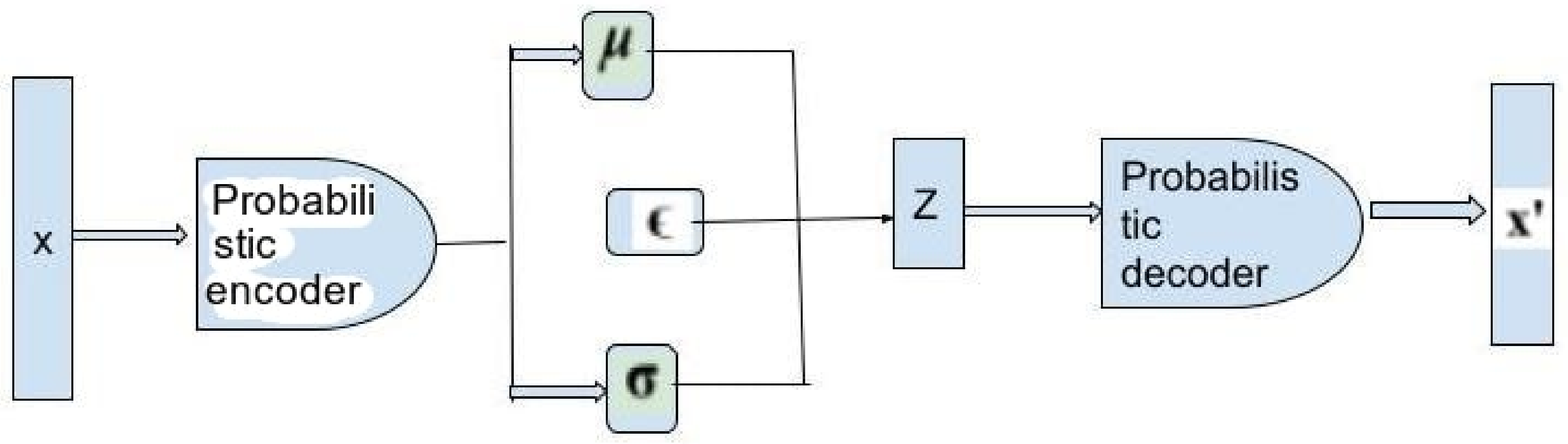
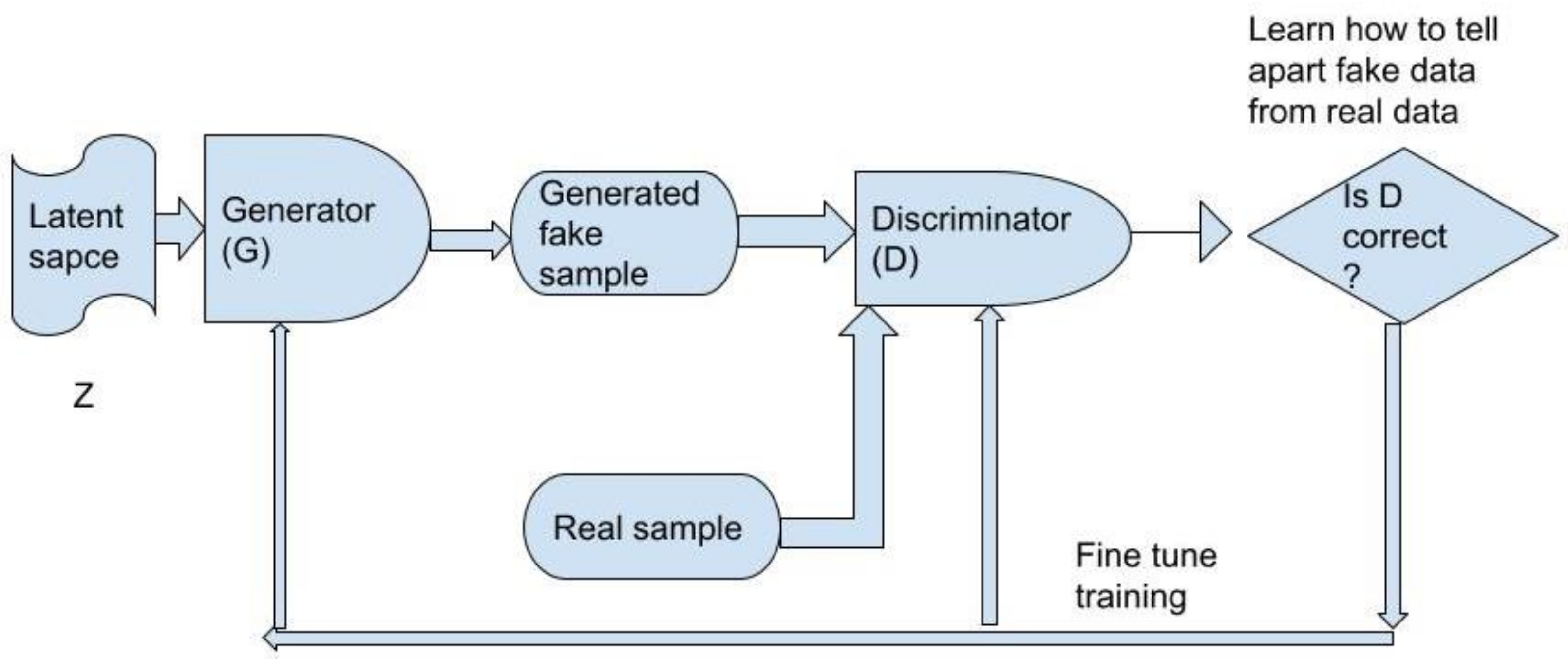
Methods for Deep Generative Model

Various deep learning techniques have been used for molecule generation, but the generative adversarial network and variational autoencoder are the two most common models. In this section, we will discuss various generative models.

Autoencoders (AEs) are neural networks that comprise two parts: one is the encoder and other is the decoder. The encoder reduces the dimension of the training sample to a latent vector and the decoder tries to reconstruct the input from latent representation. We train this AE to learn to reduce the reconstruction loss [87]. In VAEs (variational autoencoders), we use a probabilistic encoder and decoder. The encoder is a neural network that takes inputs (x) and provides a hidden representation z as an output. z has fewer dimensions than x. The encoder transforms the data it receives into a set of means and standard deviations or the parameters of a multivariate statistical distribution. Then, we sample points from this distribution and feed them to the decoder. The decoder tries to reconstruct the data (Figure 6). The objective function used for training has two terms; one is used for penalizing reconstruction errors and another is used for restricting the parameters encoded to be close to a normal distribution [88]. The loss function of the VAE is

$$\Vert x-\widehat{x}{\Vert }^2+KL[N({\mu }_x,{\sigma }_x),N(0,I)]$$

Generative adversarial networks (GANs) [89] have two components: one is the generator and the other is the discriminator. We train the generator (G) to generate a new sample and the discriminator (D) tries to classify examples as either real (from the domain) or fake (generated). The generator tries to fool the discriminator and the discriminator tries to beat the generator by performing correct classification between real and fake data. Therefore, the generator and discriminator play a game and the game goes on until it reaches an equilibrium point (Figure 7). The loss function used in a GAN is

$$\underset{G}{min}\underset{D}{max}L(D;G)=E_{x\sim p_{data}}\left[logD\left(x\right)\right]+E_{z\sim p\left(z\right)}[log(1-D\left(G\left(z\right)\right)]$$

GANs sometimes face problems like mode collapse. To avoid this, f-GAN [90] and Wasserstein-GAN [91] adopt techniques such as f-divergence for measuring the distribution distance and Wasserstein distance between distributions, respectively. There are other types of GAN, such as cyclic-GAN, StyleGAN, and StyleGAN2, which have been used widely in picture generation.

An autoregressive (AR) model forecasts future behavior using data from the past. When there is a correlation between the values in a time series, it is useful for predicting future behavior from past data. In fact, the word autoregressive comes from the fact that it only utilizes past data to model behavior. We also use this AR model for graph structure data. We assume that the graph structure data have d subcomponents and such subcomponents can have underlying dependence. For molecular graph data, the subcomponents can be nodes and bonds. The joint distribution of x is learned by factorizing it as the product of d subcomponent likelihoods, as shown below

$$P\left(x\right)=\prod _{i=1}^{d}P(x_i\mid \overline{x_1},\overline{x_2},...,\overline{x_{i-1}})$$

ARs model the joint distribution in an autoregressive or sequential fashion, anticipating the next subcomponent based on the previous subcomponents (either heuristically or with domain knowledge). A recurrent neural network is an example of an AR model.

Normalizing flows map a simple probability distribution to a complex one (learned from data). Take X as the input variable and Y as the latent variable, both of dimension n. The bijective function f that maps X and Y should be deterministic and invertible such that $X=f\left(Y\right)$ and $Y=f^{-1}\left(X\right)$. Using a change of variables, we obtain $p\left(x\right)$ as:

$$p_X\left(x\right)=p_Y\left(f^{-1}\left(x\right)\right)\left|\det \left(\frac{\partial f^{-1}\left(x\right)}{\partial x}\right)\right|$$

The determinant should be easily computable and differentiable. It is called a normalizing flow because applying the invertible transformation using a change of variables produces a normalized probability density and the invertible transformation can be composed together to generate more complex transformations, which would also have an invertible property. Multiple bijector functions can be composed together to produce more complex distributions by repeatedly applying a change of variables.

$$p\left(x\right)=p_Y\left[f_1^{-1}\left(f_0^{-1}\left(x\right)\right)\right]\left|\det \left[J_{f_1^{-1}}\right]\right|\left|\det \left[J_{f_0^{-1}}\right]\right|$$

where $J_{f_n^{-1}}$ is the determinant of the Jacobian matrix of $f_n^{-1}$ and x can be found using $f_0\left(f_1\left(y\right)\right)$. The loss function is given as:

$$l=-\log p_Y\left[f_1^{-1}\left(f_0^{-1}\left(x\right)\right)\right]-\sum _i\log \left|\det \left[J_{f_i^{-1}}\right]\right|$$

Diffusion models systematically add Gaussian noise to the training data points and learn to recover the data from noisy training data. After training the model, we can generate data from random noise data. Unlike VAEs, we aim to model a series of noise distributions in a Markov chain and reverse the noise from the data in a successive manner.

The training process is split into two steps: a forward diffusion process and learning to reverse the added noise systematically. The forward diffusion process can be represented as a Markov chain of T steps, and since it is a Markov chain, the probability density at any given time t can be computed using only the probability density at $t-1$. The resultant probability distribution is isotropic Gaussian noise.

$$q\left(x_t\right|x_{t-1})=\mathcal{N}(x_t;\sqrt{1-{\beta }_t}{x}_{t-1},{\beta }_{t}I)$$

For the reverse process, construction of data (t-1) from noise (t) requires information in respect of all previous states, to which we do not have access; hence, the neural network is trained to approximate $p_{\theta }\left(x_{t-1}\right|x_t)$ using learned parameters $\theta$.

$$p_{\theta }\left(x_{t-1}\right|x_t)=\mathcal{N}\left(x_{t-1};{\mu }_{\theta }(x_t,t),\sum _{\theta }(x_t,t)\right)$$

The loss function of the diffusion models is

$$\mathcal{L}=E_q\left(-\log p\left(x_T\right)-\sum _{t\ge 1}\log \frac{p_{\theta }\left(x_{t-1}\right|x_t)}{q\left(x_t\right|x_{t-1})}\right)$$

Similarly, there are other generative models, e.g., energy-based models (EBMs).

8. Design of Kinase Inhibitors Using CADD

This section will discuss the progress of designing kinase inhibitors using CADD. Significant research has been performed on the design of kinase inhibitors using computer-aided drug design (CADD) techniques. CADD techniques have allowed for identifying potential inhibitors and optimizing their structures more efficiently and cost-effectively than traditional experimental methods. Researchers have used various CADD techniques to design kinase inhibitors, including molecular docking, virtual screening, molecular dynamics simulations, and machine learning algorithms. These techniques have been used to predict potential inhibitors’ binding affinity, selectivity, and pharmacokinetic properties, and to optimize their chemical structures to improve their efficacy and safety. Overall, using CADD techniques in the design of kinase inhibitors has led to significant advances in drug discovery and has enabled the development of targeted and effective drugs for treating various diseases. Ongoing research in this field is focused on developing new CADD techniques and optimizing existing ones to accelerate the drug discovery process further and improve the success rates of clinical trials. Several studies have shown the successful application of CADD techniques in designing kinase inhibitors for treating cancer, inflammation, and other diseases. One study published in the Journal of Medicinal Chemistry used molecular docking and molecular dynamics simulations to design potent and selective inhibitors of the receptor tyrosine kinase, c-Met [92]. The inhibitors showed high binding affinity and selectivity for c-Met and inhibited the growth of cancer cells in vitro. Another study published in ACS Chemical Biology used a combination of virtual screening and molecular dynamics simulations to design selective inhibitors of the protein kinase, Aurora-A [93]. The inhibitors showed high binding affinity and selectivity for Aurora-A and inhibited the growth of cancer cells in vitro. Additionally, CADD techniques have been used to identify and optimize inhibitors of other kinases, such as EGFR, BRAF, and PI3K, which are commonly mutated in various types of cancer. One example of a successful application of CADD techniques in kinase inhibitor design is the development of Imatinib, a drug used to treat chronic myeloid leukemia (CML) [94]. Imatinib was developed by Novartis in the early 2000s using molecular modeling and crystallography to design a small molecule inhibitor that specifically targeted the BCR-ABL kinase associated with CML [95]. Imatinib has since become a first-line therapy for CML and has also shown promising results in other cancers. Another example of the application of CADD techniques in kinase inhibitor design is the development of ABL kinase inhibitors for the treatment of non-small cell lung cancer (NSCLC). Researchers have used molecular docking and molecular dynamics simulations to design inhibitors that can target the mutant forms of ABL kinase that are associated with NSCLC. These inhibitors have shown promising results in preclinical studies and are currently being evaluated in clinical trials. One study used molecular docking and virtual screening to identify potential inhibitors of the Janus kinase 3 (JAK3) enzyme, which is involved in autoimmune diseases. The researchers identified several compounds with high binding affinity and selectivity for JAK3, which were then experimentally validated as potent inhibitors [96]. In another study, researchers used molecular dynamics simulations to study the binding of potential inhibitors to the protein kinase p38, which is involved in inflammation [97]. The simulations provided insights into the stability and flexibility of the inhibitor–target complex, which were used to optimize the chemical structure of the inhibitor. One example is a study published in the Journal of Medicinal Chemistry, which used molecular docking and virtual screening to identify potential inhibitors of the protein kinase A (PKA) enzyme. The researchers screened a large database of compounds and identified several potential inhibitors with high binding affinity for PKA. The compounds were then experimentally validated and shown to be effective inhibitors of PKA activity. In another study, published in ACS Chemical Biology, researchers used molecular dynamics simulations to study the binding of potential inhibitors to the epidermal growth factor receptor (EGFR), which is involved in cancer. The simulations provided insights into the interactions between the inhibitor and the receptor, which were used to optimize the chemical structure of the inhibitor. The optimized inhibitor was shown to be more potent than the original compound in inhibiting EGFR activity. Another study used virtual screening to identify potential inhibitors of the protein kinase B (AKT) enzyme, which is involved in cancer [98]. The researchers screened a library of over 2 million compounds and identified several potential inhibitors with high binding affinity for AKT. The most promising compound was then optimized using structure-based design, resulting in a potent and selective AKT inhibitor [98]. In another study, researchers used molecular dynamics simulations to study the binding of potential inhibitors to the protein kinase CK2, which is involved in various cancers [99]. The simulations provided insights into the binding mechanism and stability of the inhibitor–target complex, which were used to optimize the chemical structure of the inhibitor. Molecular dynamics has also been used to identify potential inhibitors of the protein kinase Cdc7, which is involved in cancer cell proliferation [100]. These studies demonstrate the power of CADD techniques in the design of kinase inhibitors, allowing for the identification and optimization of compounds with high binding affinity and selectivity. These techniques can significantly accelerate the drug discovery process and lead to the development of more effective and targeted drugs for the treatment of various diseases. As computational power and simulation methods continue to improve, it is expected that CADD techniques will become even more powerful in the design of new drugs to treat a wide range of diseases.

9. Evaluation Methods for Different Machine Learning and Deep Learning Generative Techniques for Drug Design

Molecule generation evaluation methods provide insight into model performance depending on the type of evaluation metric used (

Table 2. ML performance evaluation methods.

ML Models	Performance Analysis Metric
Linear regression	RMSE
Logistic regression	RMSE
SVM	Accuracy or F-1 score
Q-learning	Cumulative reward
R-learning	IQM on performance profiles

), and some of these methods could also be used for the loss function of back-propagation. Different evaluation methods produce different classes of results of varying impacts and it is important to understand the various evaluation methods and choose the right one in order to benchmark a deep learning model for the goal in mind.

9.1. Simple Numeric Methods

These are simple numeric evaluation methods based on the generated molecules and training dataset molecules.

• Validity [101] is the ratio of valid molecules to the total number of molecules in the generated molecules dataset. A valid molecule is one where all atoms’ corresponding bonds match their valency and validity estimates the model’s ability to learn the valency of atoms.

  $$\mathrm{Validity}=\frac{\left|\mathrm{valid}\mathrm{molecules}\right|}{\left|\mathrm{total}\mathrm{generated}\mathrm{molecules}\right|}$$
• Novelty [101] is the ratio of molecules that do not appear in the training set to the total number of molecules in the generated molecules dataset. It estimates the ability of the model to tap into the unknown chemical space.

  $$\mathrm{Novelty}=\frac{\left|\mathrm{novel}\mathrm{molecules}\right|}{\left|\mathrm{total}\mathrm{generated}\mathrm{molecules}\right|}$$
• Uniqueness [101] is the ratio of unique molecules to the total number of molecules in the generated molecules dataset. It estimates the generative repetitiveness of a model and a high unique score is ideal.

  $$\mathrm{Uniqueness}=\frac{\left|\mathrm{unique}\mathrm{molecules}\right|}{\left|\mathrm{total}\mathrm{generated}\mathrm{molecules}\right|}$$
• Diversity [102] is classified into two categories: internal diversity (IntDiv) and external diversity (ExtDiv). IntDiv is the measure of similarity between molecules in the generated molecules dataset. ExtDiv is the measure of similarity between molecules in the generated molecules dataset and the training dataset. It uses the power (p) mean of the pairwise Tanimoto similarity (S) between the generated (G) dataset and the training (T) dataset.

  $$\mathrm{IntDiv}=1-\sqrt[p]{\frac{1}{{\left|\mathrm{G}\right|}^2}\sum _{g1,g2\in G}S{(g1,g2)}^p}$$

  $$\mathrm{ExtDiv}=1-\sqrt[p]{\frac{1}{\left|\mathrm{G}\right|\left|\mathrm{T}\right|}\sum _{g\in G,t\in T}S{(g,t)}^p}$$

9.2. Probabilistic Distribution Methods

Evaluation methods that compare the probability distributions of the training and generated molecules dataset.

• Kullback–Leibler Divergence (KL-Divergence) [103] is a measure of the statistical distance between two probability distributions of various physicochemical descriptors from the training and generated molecules datasets. A low KLD for any descriptor implies the model has successfully learned its distribution. The formula for KLD for a descriptor (D) between the generated (G) and training (T) distribution is shown:

  $${\mathrm{D}}_{\mathrm{KL}}(\mathrm{G},\mathrm{T};\mathrm{D})=\sum _i\mathrm{G}\left(\mathrm{i}\right)\log \frac{G\left(i\right)}{T\left(i\right)}$$
• Frechet ChemNet Distance (FCD) [104] uses the means ($\mu$) and covariances (C) of the features of the training (T) and generated (G) datasets from the penultimate layer of ChemNet. Lower values are better as they imply the distributions are closer.

  $$\mathrm{FCD}(\mathrm{G},\mathrm{T})=\mid \mid {\mu }_G-{\mu }_T\mid {\mid }^2+Tr(C_G+C_T-2{\left(C_G{C}_T\right)}^{1/2})$$

9.3. Optimization Evaluation Methods

Optimization methods are used to generate molecules with specific properties. Following are some properties that are optimized and only require the molecule as input:

1.

Synthetic accessibility score (SAS) [105] is a value used to estimate the ease of synthesis of a molecule. A low score implies ease in the synthesis of the drug-like molecule. Its range is from 0 to 10.

2.

Quantitative Estimate of Drug-likeness (QED) [106] is used to calculate the drug-likeness of a molecule using descriptors from various drugs in the market, and is calculated by taking the geometric mean of all the desirable functions, each corresponding to different descriptors. Its range is from 0 to 1.

3.

Octanol–water partition coefficient (LogP) [107] is used to calculate how hydrophobic/hydrophilic a molecule is. Its range is on average from −3 to 7.

$$\log \left(P_{oct/wat}\right)={\log }_{10}\left(\frac{{\mathrm{solute}}_{\mathrm{octanol}}^{\mathrm{unionized}}}{{\mathrm{solute}}_{\mathrm{water}}^{\mathrm{unionized}}}\right)$$

4.

Topological polar surface area (TPSA) [108] calculates the molecular polar surface area of the polar atoms, which provides insight into the transport properties of drugs.

5.

GuacaMol [103] is a benchmarking suite for drug-like molecules that uses 5 distribution-learning benchmarks (novelty, validity, uniqueness, KLD, and FCD) and 20 goal-directed benchmarks (e.g., Scaffold Hop, Valsartan SMARTS, Celecoxib rediscovery, Albuterol similarity, Median molecules, Osimertinib MPO).

6.

Vina [109] is a scoring function that measures the protein–ligand binding affinity by summing the important energy factors in protein–ligand binding.

7.

Celecoxib rediscovery [110] is a rediscovery method that attempts to rediscover the target molecule when removed from the training dataset. Its range lies from 0 to 1.

9.4. 3D Similarity Methods

In the 3D space, one molecule could have many conformations and it is essential to find the right conformation as the protein binding pocket is structure-based. Hence, we need a specific conformation for the targeted protein pocket.

• Root-mean-squared deviation [111] calculates the 3D alignment similarity between two molecule conformations from training set $R\in {\mathbb{R}}^{3\mathrm{x}n}$ and generated molecule $R^{\prime }\in {\mathbb{R}}^{3\mathrm{x}n}$. $R^{\prime }$ is found by rotating and translating the original conformation $R_g$ to obtain RMSD(R,R’).

  $$RMSD(R,R^{\prime })=\sqrt{\frac{1}{n}\sum _{i=1}^n\mid \mid R_i-R_i^{\prime }\mid {\mid }^2}$$
• SHApeFeaTure Similarity (SHAFTS) [112] uses a hybrid similarity method using molecular shape and chemical groups appended by pharmacophore features for 3D similarity calculation. The hybrid similarity has two parts: shape-density overlap (ShapeScore) is the intersection between two molecules A and B, which is the sum of the overlap integrals of single atomic shape-densities for which a Gaussian function was used. $d_{ij}$ is the interatomic distance.

  $$V_{AB}=\sum _{i\in A}\sum _{j\in B}\int d\overrightarrow{r}{\rho }_i\left(\overrightarrow{r}\right){\rho }_j\left(\overrightarrow{r}\right)$$

  $$ShapeScore=\frac{V_{AB}}{\sqrt{V_A{V}_B}}$$
• FeatureScore is the sum of overlap between the feature points in A and B of the same type. $d_{ij}$ is the distance between the features of A and B and $R_f$ is the overlap tolerance.

  $$F_{AB}=\sum _{f\in F}\sum _{i\in A}\sum _{j\in B}exp\left[-2.5{\left(\frac{d_{ij}}{R_f}\right)}^2\right]$$

  $$FeatureScore=\frac{F_{AB}}{\sqrt{F_A{F}_B}}$$
• Finally, the hybrid score is defined as a weighted sum of the ShapeScore and FeatureScore scaled to [0, 2].

  $$HybridScore=ShapeScore+FeatureScore$$
• Rapid overlay of chemical structures (ROCS) [113] uses unweighted sums to aggregate many features of similarity, resulting in parameter-free models. It measures the chemical and shape similarity of two molecules by calculating the Tanimoto coefficients of the aligned overlap volumes:

  $$T(A,B)=\frac{O_{AB}}{O_{AA}+O_{BB}-O_{AB}}$$

10. Drug Development Database

In last few decades, researchers have created multiple large-scale databases to enhance computational drug discovery projects (

Table 3. Different datasets used for drug discovery task.

Dataset	Approximate Amount	Description
QM9 [114,115]	134,000	This is a subset of GDB-13 (a database of nearly 1 billion stable and synthetically accessible organic molecules) composed of all molecules of up to 23 atoms including 9 heavy atoms. QM9 provides quantum chemical properties for the chemical space of small organic molecules.
ZINC [116]	250,000	It comprises over 230 million compounds in ready-to-dock, 3D formats.
Molecular Sets (MOSES) [117]	1,937,000	The set is based on the ZINC Clean Leads collection. This dataset has been filtered from the ZINC dataset. These are the drug-like molecules.
ChEMBL [118]	2,100,000	A database of bioactive compounds with drug-like molecules, which is manually curated.
GDB13 [119]	970,000,000	In this dataset, we have small organic compounds with up to 13 atoms, using chemical stability and synthetic feasibility principles. It is the largest publicly available small organic molecule database.
GEOM-QM9 [120]	450,000; 37,000,000	The 3D conformer ensembles are annotated by GEOM-QM9 using sophisticated sampling and semiempirical density functional theory. The dataset contains around 133K 3D molecules.
GEOM-Drugs [120]	317,000	This dataset also uses advanced sampling and semiempirical density functional theory to annotate the 3D conformer ensembles.
ISO17 [121]	200; 431,000	This dataset contains 197 2D molecules and 430,692 molecule-conformation pairs.
Molecule3D [122]	4 million	This dataset contains almost 4 million molecules and researchers use density functional theory to create exact ground-state geometries for the molecules in the dataset.
CrossDock2020 [123]	22,500,000	The CrossDocked2020 collection contains 22.5 million docked ligand poses in various binding pockets that are similar across the Protein Data Bank.
scPDB [124]		An annotated database of druggable binding sites from the Protein Data Bank. It registers 9283 binding sites from 3678 unique proteins and 5608 unique ligands, with a total of 16,034 entries.
DUD-E [125]		DUD-E contains 102 target-specific affinity scores and 22,886 active molecules.

). QM9 [114,115], ZINC [116], Molecular Sets (MOSES) [117], ChEMBL [118], and GDB13 [119] are the datasets generally used for 1D/2D molecule generation and optimization. In drug discovery projects, researchers use smile string (1D data) or graph data (2D data) but molecules have a 3D structure by nature. Therefore, 1D or 2D data process less information than 3D data. For drug discovery, molecules’ 3D structures are crucial to their activities in a variety of applications, including molecular dynamics and docking. The purpose of 3D molecule production is to create molecules in three dimensions. One 1D/2D molecule has a variety of 3D geometries or conformations, unlike 1D/2D molecule production. This yields a list of tasks, the end outputs of which should be 3D molecules. GEOM-QM9 [120], GEOM-Drugs [120], ISO17 [121], Molecule3D [122], CrossDock2020 [123], scPDB [124], and DUD-E [125] are the datasets generally used for 3D molecule generation.

11. Discussion

We have given a detailed description of the traditional state-of-the-art methods of CADD, along with the related new advanced techniques. Computational drug design (CADD) has significant theoretical and clinical importance over the traditional drug development process. Here are some key points:

Theoretical Importance:

Speed and Efficiency: CADD allows for the rapid screening of large libraries of compounds, reducing the time and cost involved in drug development.

Precision and Control: CADD offers greater precision and control over molecular properties, enabling the design of drugs with specific, desired characteristics. This is important for targeting specific disease mechanisms and minimizing off-target effects.

Insights into Molecular Mechanisms: CADD can provide detailed insights into the interactions between drugs and their targets at the molecular level, helping researchers to understand the mechanisms of action of drugs and to optimize their properties.

Reduction of Animal Testing: CADD can help reduce the need for animal testing by providing information about the biological activity and toxicity of drug candidates before they are tested in vivo.

Clinical Importance:

Identification of Effective Drugs: CADD can help identify drug candidates with a higher likelihood of success, increasing the chances of developing effective drugs for treating diseases.

Reduced Adverse Effects: CADD can help minimize adverse effects by designing drugs that are highly specific to their targets, reducing the risk of unintended interactions with other molecules in the body.

Personalized Medicine: CADD can help facilitate the development of personalized medicine by allowing for the design of drugs tailored to specific patient needs, such as individual genetic variations.

Improved Patient Outcomes: CADD can help improve patient outcomes by enabling the development of more effective drugs with fewer adverse effects.

In summary, CADD offers several theoretical and clinical advantages over the traditional drug development process. By providing greater precision, efficiency, and control over drug design, CADD has the potential to accelerate drug development, improve drug efficacy and safety, and reduce the costs associated with traditional drug design methods.

However, CADD has its own challenges [126,127,128,129,130]. We summarize below the challenges in respect of CADD, from traditional methods to molecule generation using deep learning. SBDD is the most promising technique in drug design but still it has some limitations. Challenges regarding the chemical space are as follows:

• Expand the chemical space that is medically relevant.
• Design and screen extremely large chemical libraries rationally.
• Extract lead compounds and unknown hits from screening libraries.

Challenges regarding the biological space are as follows:

• Improve multi-target drug design.
• Identify responsible region in genome.
• Improve targeting protein–protein interaction module.

Challenges regarding methods are as follows:

• Try to reduce off-target binding during clinical trials.
• For multi-target drug design, reduce toxicity.
• Compound and library enumeration.
• Improve medically relevant 3D drug molecule design.
• In molecule generation methods using deep learning we face many challenges, such as out-of-distribution generation, lack of interoperability, lack of unified evaluation protocol, generation in low-data regime, etc.

Researchers are trying to solve these challenges and we hope that deep learning will take drug design to the next level in the coming decade.

12. Conclusions

In this study, we reviewed the computational drug design process. Computational drug design is a field that uses computational tools and techniques to design and optimize drug molecules with specific therapeutic properties. CADD has become an essential part of the drug discovery and development process, allowing researchers to save time and resources by rapidly identifying potential drug candidates that can be further tested in a laboratory. There are several steps involved in the computational drug design process. First, the target protein or biological system with which the drug is meant to interact is identified. This can be achieved through various methods, including bioinformatics, structural biology, and molecular modeling. Once the target is identified, the next step is to generate or identify potential drug candidates. This is typically achieved using a combination of virtual screening, molecular docking, and molecular dynamics simulations. Virtual screening involves the use of computer algorithms to screen large databases of chemical compounds and identify molecules that have the potential to interact with the target protein. Molecular docking involves predicting the binding affinity and orientation of potential drug molecules to the target protein, while molecular dynamics simulations are used to predict the dynamic behavior of the drug–target complex. Once potential drug candidates are identified, they are further optimized through various computational methods, such as structure-based design, ligand-based design, and fragment-based design. Structure-based design involves using the known structure of the target protein to design molecules that will interact with specific regions of the protein. Ligand-based design involves optimizing the chemical structure of a known drug molecule to improve its activity and specificity. Fragment-based design involves using small fragments of molecules to design larger drug molecules. Overall, computational drug design has become an essential tool in the drug discovery and development process, allowing researchers to rapidly identify and optimize potential drug candidates. While there are still limitations to the accuracy of computational methods, the field continues to evolve and improve, leading to new and innovative drug discoveries. Lastly, it is important to note that computational drug design is not a replacement for traditional drug discovery methods. Rather, it is a complementary tool that can help researchers to identify potential and effective drug candidates. Moreover, the ultimate goal of future work is to utilize a combination of computational approaches and experimental wet lab-based experiments together to identify and develop safe and effective drugs for the treatment of various complex diseases for the benefit of human beings and public health services.

References

- Parvu, L. QSAR—A piece of drug design. J. Cell Mol. Med. 2003, 7, 333–335. [Google Scholar] [CrossRef] [PubMed]
- Duong-Ly, K.C.; Peterson, J.R. The human kinome and kinase inhibition. Curr. Protoc. Pharmacol. 2013, 60, 2–9. [Google Scholar] [CrossRef] [PubMed]
- Bhullar, K.S.; Lagarón, N.O.; McGowan, E.M.; Parmar, I.; Jha, A.; Hubbard, B.P.; Rupasinghe, H.V. Kinase-targeted cancer therapies: Progress, challenges and future directions. Mol. Cancer 2018, 17, 1–20. [Google Scholar] [CrossRef] [PubMed]
- Chandrasekaran, B.; Abed, S.N.; Al-Attraqchi, O.; Kuche, K.; Tekade, R.K. Chapter 21—Computer-Aided Prediction of Pharmacokinetic (ADMET) Properties. In Dosage Form Design Parameters; Academic Press: Cambridge, MA, USA, 2018; pp. 731–755. [Google Scholar]
- Lengauer, T.; Rarey, M. Computational methods for biomolecular docking. Curr. Opin. Struct. Biol. 1996, 6, 402–406. [Google Scholar] [CrossRef] [PubMed]
- Fefpia, M.; Marshall, S.; Burghaus, R.; Cosson, V.; Cheung, S.; Chenel, M.; Dellapasqua, O.; Frey, N.; Hamrén, B.; Harnisch L., T. Good Practices in Model-Informed Drug Discovery and Development Practice Application and Documentation. CPT Pharm. Syst. Pharmacol. 2016, 5, 93–122. [Google Scholar]
- Ghosh, B.; Choudhuri, S.T. Drug Design for Malaria with Artificial Intelligence (AI). In Plasmodium Species and Drug Resistance; IntechOpen: London, UK, 2021. [Google Scholar]
- Mullard Asher, T. Biotech R&D spend jumps by more than 15%. Nat. Rev. Drug Discov. 2016, 15, 447–448. [Google Scholar]
- Choudhuri, S.; Mallik, S.; Ghosh, B.; Si, T.; Bhadra, T.; Maulik, U.; Li, A. A Review of Computational Learning and IoT Applications to High-Throughput Array-Based Sequencing and Medical Imaging Data in Drug Discovery and Other Health Care Systems. In Applied Smart Health Care Informatics: A Computational Intelligence Perspective; John Wiley & Sons: New York, NY, USA, 2022. [Google Scholar]
- Barabási, A.L.; Gulbahce, N.; Loscalzo, J. Improved protein structure prediction using potentials from deep learning. Nature 2020, 577, 706–710. [Google Scholar]
- Berman, H.M.; Westbrook, J.; Feng, Z.; Gilliland, G.; Bhat, T.N.; Weissig, H.; Shindyalov, I.N.; Bourne, P.E. The Protein Data Bank. Nucleic Acids Res. 2000, 28, 235–242. [Google Scholar] [CrossRef] [PubMed]
- Laurie, A.T.; Jackson, R.M. Q-sitefinder An energy-based method for the prediction of protein-ligand binding sites. Bioinformatics 2005, 21, 1908–1916. [Google Scholar] [CrossRef] [PubMed]
- Ewing, T.J.; Makino, S.; Skillman, A.G.; Kuntz, I.D. search strategies for automated molecular docking of flexible molecule databases. J. Comput. Aided Mol. Des. 2001, 15, 411–428. [Google Scholar] [CrossRef]
- Goodsell, D.S.; Olson, A.J. Automated docking of substrates to proteins by simulated annealing. Proteins 1990, 8, 195–202. [Google Scholar] [CrossRef]
- Wang, J.; Wolf, R.M.; Caldwell, J.W.; Kollman, P.A.; Case, D.A. Development and testing of a general amber force field. J. Comput. Chem. 2004, 25, 1157–1174. [Google Scholar] [CrossRef] [PubMed]
- Vanommeslaeghe, K.; Hatcher, E.; Acharya, C.; Kundu, S.; Zhong, S.; Shim, J.; Darian, E.; Guvench, O.; Lopes, P.; Vorobyov, I.; et al. CHARMM general force field a force field for drug-like molecules compatible with the CHARMM all-atom additive biological force fields. J. Comput. Chem. 2010, 31, 671–690. [Google Scholar] [CrossRef]
- Cournia, Z.; Chipot, C.; Roux, B.; York, D.M.; Sherman, W. Free Energy Methods in Drug Discovery—Introduction. ACS Symp. Ser. 2021, 1397, 1–38. [Google Scholar]
- Hou, T.; Wang, J.; Li, Y.; Wang, W. Assessing the performance of the MM/PBSA and MM/ GBSA methods. 1. The accuracy of binding free energy calculations based on molecular dynamics simulations. J. Chem. Inf. Model. 2010, 51, 69–82. [Google Scholar] [CrossRef] [PubMed]
- Hansson, T.; Marelius, J.; Åqvist, J. Ligand binding affinity prediction by linear interaction energy methods. J. Comput. Aided Mol. Des. 1998, 12, 27–35. [Google Scholar] [CrossRef] [PubMed]
- Kandel, J.; Tayara, H.; Chong, K.T. PUResNet prediction of protein-ligand binding sites using deep residual neural network. J. Cheminform. 2021, 13, 65. [Google Scholar] [CrossRef] [PubMed]
- Ahmed, A.; Mam, B.; Sowdhamini, R. A Deep Learning Approach to Predict Protein-Ligand Binding Affinity. Bioinform. Biol. Insights 2021, 15, 11779322211030364. [Google Scholar] [CrossRef]
- Eramian, M.Y.S.; Pieper, U.; Sali, A. Comparative protein structure modeling using MODELLER. Curr. Protoc. Protein Sci. 2006, 5, 6. [Google Scholar]
- Schwede, T.; Kopp, J.; Guex, N.; Peitsch, M.C. SWISS-MODEL an automated protein homology-modeling server. Nucleic Acids Res 2003, 31, 3381–3385. [Google Scholar] [CrossRef] [PubMed]
- Bernard, D.; Coop, A.; MacKerell, A.D., Jr. Conformationally sampled pharmacophore for peptidic delta. J. Med. Chem. 2005, 48, 73–80. [Google Scholar] [CrossRef]
- Duchowicz, P.R.; Castro, E.A.; Fernández, F.M.; Gonzalez, M.P. A new search algorithm of QSPR/QSAR theories Normal boiling points of some organic molecules. Chem. Phys. Lett. 2005, 412, 376–380. [Google Scholar] [CrossRef]
- Wade, R.C.; Henrich, S.; Wang, T.T. Using 3D protein structures to derive 3D-QSARs. Drug Discov. Today Technol. 2004, 1, 241–246. [Google Scholar] [CrossRef] [PubMed]
- Acharya, C.; Coop, A.; Polli, J.E.; Mackerell, A.D., Jr. Recent advances in ligand-based drug design relevance and utility of the conformationally sampled pharmacophore approach. Curr. Comput. Aided Drug Des. 2011, 7, 11–22. [Google Scholar] [CrossRef] [PubMed]
- Bohl, C.E.; Chang, C.; Mohler, M.L.; Chen, J.; Miller, D.D.; Swaan, P.W.; Dalton, J.T. A ligand-based approach to identify quantitative structure-activity relationships for the androgen receptor. J. Med. Chem. 2004, 47, 3765–3776. [Google Scholar] [CrossRef]
- Winkler David Alan, T. Overview of Quantitative Structure—Activity Relationships (QSAR). In Molecular Analysis and Genome Discovery; John Wiley & Sons: New York, NY, USA, 2004; pp. 347–367. [Google Scholar]
- Topliss, J.G.; Edwards, R.P.T. Chance factors in studies of quantitative structure-activity relationships. J. Med. Chem 1979, 22, 1238–1244. [Google Scholar] [CrossRef] [PubMed]
- Hawkins, D.M.; Basak, S.C.; Shi, X. QSAR with few compounds and many features. J. Chem. Inform. Comput. Sci. 2001, 41, 663–670. [Google Scholar] [CrossRef] [PubMed]
- Gleeson, M.P.; Modi, S.; Bender, A.; Robinson, R.L.M.; Kirchmair, J.; Promkat, T. The challenges involved in modeling toxicity data in silico a review. Curr. Pharm. Des. 2012, 18, 1266–1291. [Google Scholar] [CrossRef] [PubMed]
- Pujol, A.; Mosca, R.; Farrés, J.; Aloy, P. Unveiling the role of network and systems biology in drug discovery. Trends Pharmacol. Sci. 2010, 31, 115–123. [Google Scholar] [CrossRef]
- Butcher, E.C.; Berg, E.L.; Kunkel, E.J. Systems biology in drug discovery. Nat. Biotechnol. 2004, 22, 1253–1259. [Google Scholar] [CrossRef]
- Barabási, A.L.; Gulbahce, N.; Loscalzo, J. Network medicine a network-based approach to human disease. Nat. Rev. Genet. 2011, 12, 56–68. [Google Scholar] [CrossRef] [PubMed]
- Lim, J.; Ryu, S.; Kim, J.W.; Kim, W.Y. Molecular generative model based on conditional variational autoencoder for de novo molecular design. J. Cheminform. 2018, 10, 1–9. [Google Scholar] [CrossRef] [PubMed]
- Kang, S.; Cho, K. Conditional molecular design with deep generative models. J. Chem. Inf. Model. 2018, 59, 43–52. [Google Scholar] [CrossRef]
- Harel, S.; Radinsky, K. Prototype-based compound discovery using deep generative models. Mol. Pharm. 2018, 15, 4406–4416. [Google Scholar] [CrossRef] [PubMed]
- Gómez-Bombarelli, R.; Wei, J.N.; Duvenaud, D.; Hernández-Lobato, J.M.; Sánchez-Lengeling, B.; Sheberla, D.; Aguilera-Iparraguirre, J.; Hirzel, T.D.; Adams, R.P. Automatic chemical design using a data-driven continuous representation of molecules. ACS Cent. Sci. 2018, 4, 268–276. [Google Scholar] [CrossRef]
- Blaschke, T.; Olivecrona, M.; Engkvist, O.; Bajorath, J.; Chen, H. Application of generative autoencoder in de novo molecular design. Mol. Inform. 2017, 37, 1700123. [Google Scholar] [CrossRef] [PubMed]
- Sattarov, B.; Baskin, I.I.; Horvath, D.; Marcou, G.; Bjerrum, E.J.; Varnek, A. De novo molecular design by combining deep autoencoder recurrent neural networks with generative topographic mapping. J. Chem. Inf. Model. 2019, 59, 1182–1196. [Google Scholar] [CrossRef]
- Kusner, M.J.; Paige, B.; Hernández-Lobato, J.M. Grammar Variational Autoencoder. arXiv 2017, arXiv:1703.01925. [Google Scholar]
- Jørgensen, P.B.; Mesta, M.; Shil, S.; García Lastra, J.M.; Jacobsen, K.W.; Thygesen, K.S.; Schmidt, M.N. Machine learning-based screening of complex molecules for polymer solar cells. J. Chem. Phys. 2018, 148, 241735. [Google Scholar] [CrossRef]
- Jørgensen, P.B.; Schmidt, M.N.; Winther, O. Deep generative models for molecular science. Mol. Inform. 2018, 37, 1700133. [Google Scholar] [CrossRef] [PubMed]
- Dai, H.; Tian, Y.; Dai, B.; Skiena, S.; Song, L. Syntax-directed variational autoencoder for structured data. arXiv 2018, arXiv:1802.08786. [Google Scholar]
- Liu, Q.; Allamanis, M.; Brockschmidt, M.; Gaunt, A. Constrained graph variational autoencoders for molecule design. arXiv 2018, arXiv:1805.09076. [Google Scholar]
- Samanta, B.; De, A.; Ganguly, N.; Gomez-Rodriguez, M. Designing random graph models using variational autoencoders with applications to chemical design. arXiv 2018, arXiv:1802.05283. [Google Scholar]
- Winter, R.; Montanari, F.; Noé, F.; Clevert, D.A. Learning Continuous and Data-Driven Molecular Descriptors by Translating Equivalent Chemical Representations. Chem. Sci. 2019, 10, 1692–1701. [Google Scholar] [CrossRef] [PubMed]
- Kajino, H. Molecular Hypergraph Grammar with its Application to Molecular Optimization. arXiv 2018, arXiv:1803.03324. [Google Scholar]
- Jin, W.; Barzilay, R.; Jaakkola, T. Junction tree variational autoencoder for molecular graph generation. In Proceedings of the International Conference on Learning Representations, Stockholm, Sweden, 10–15 July 2018. [Google Scholar]
- Jin, W.; Yang, K.; Barzilay, R.; Jaakkola, T. Learning Multimodal Graph-to-Graph Translation for Molecular Optimization. In Proceedings of the International Conference on Learning Representations, New Orleans, LA, USA, 6–9 May 2019. [Google Scholar]
- Samanta, B.; De, A.; Jana, G.; Gómez, V.; Chattaraj, P.K.; Ganguly, N.; Gomez-Rodriguez, M. NeVAE A Deep Generative Model for Molecular Graphs. arXiv 2019, arXiv:1802.05283. [Google Scholar] [CrossRef]
- Simonovsky, M.; Komodakis, N. Graphvae Towards generation of small graphs using variational autoencoders. arXiv 2018, arXiv:1802.03480. [Google Scholar]
- Ma, T.; Chen, J.; Xiao, C. Constrained Generation of Semantically Valid Graphs via Regularizing Variational Autoencoders. In Proceedings of the Advances in Neural Information Processing Systems 32: Annual Conference on Neural Information Processing Systems 2019, NeurIPS 2019, Vancouver, BC, Canada, 8–14 December 2019. [Google Scholar]
- Skalic, M.; Jiménez, J.; Sabbadin, D.; De Fabritiis, G. Shape-based generative modeling for de-novo drug design. J. Chem. Inf. Model. 2019, 59, 1205–1214. [Google Scholar] [CrossRef] [PubMed]
- Kuzminykh, D.; Polykovskiy, D.; Kadurin, A.; Zhebrak, A.; Baskov, I.; Nikolenko, S.; Shayakhmetov, R.; Zhavoronkov, A. 3D molecular representations based on the wave transform for convolutional neural networks. Mol. Pharm. 2018, 15, 4378–4385. [Google Scholar] [CrossRef] [PubMed]
- Steven, M. Kearnes Li Li and Patrick Riley, T. Decoding molecular graph embeddings with reinforcement learning. arXiv 2019, arXiv:1904.08915. [Google Scholar]
- Guimaraes, G.L.; Sanchez-Lengeling, B.; Outeiral, C.; Farias, P.L.C.; Aspuru-Guzik, A. Objective-Reinforced Generative Adversarial Networks (ORGAN) for Sequence Generation Models. arXiv 2017, arXiv:1705.10843. [Google Scholar]
- Putin, E.; Asadulaev, A.; Ivanenkov, Y.; Aladinskiy, V.; Sanchez-Lengeling, B.; Aspuru-Guzik, A.; Zhavoronkov, A. Reinforced adversarial neural computer for de novo molecular design. J. Chem. Inf. Model. 2018, 58, 1194–1204. [Google Scholar] [CrossRef] [PubMed]
- Putin, E.; Asadulaev, A.; Vanhaelen, Q.; Ivanenkov, Y.; Aladinskaya, A.V.; Aliper, A.; Zhavoronkov, A. Adversarial threshold neural computer for molecular de novo design. Mol. Pharm. 2018, 15, 4386–4397. [Google Scholar] [CrossRef] [PubMed]
- Kadurin, A.; Nikolenko, S.; Khrabrov, K.; Aliper, A.; Zhavoronkov, A. druGAN An advanced generative adversarial autoencoder model for de novo generation of new molecules with desired molecular properties in silico. Mol. Pharm. 2017, 14, 3098–3104. [Google Scholar] [CrossRef] [PubMed]
- Méndez-Lucio, O.; Baillif, B.; Clevert, D.A.; Rouquié, D.; Wichard, J. De novo generation of hit-like molecules from gene expression signatures using artificial intelligence. Nat. Commun. 2020, 11, 10. [Google Scholar] [CrossRef] [PubMed]
- De Cao, N.; Kipf, T. MolGAN An implicit generative model for small molecular graphs. In Proceedings of the ICML 2018 Workshop on Theoretical Foundations and Applications of Deep Generative Models, Stockholm, Sweden, 14–15 July 2018. [Google Scholar]
- De Cao, N.; Kipf, T. MolGAN An implicit generative model for small molecular graphs. arXiv 2018, arXiv:1805.11973. [Google Scholar]
- Maziarka, Ł.; Pocha, A.; Kaczmarczyk, J.; Rataj, K.; Danel, T.; Warchoł, M. Mol-cyclegan—A generative model for molecular optimization. J. Cheminform. 2020, 12, 1758–2946. [Google Scholar] [CrossRef]
- Merk, D.; Friedrich, L.; Grisoni, F.; Schneider, G. De novo design of bioactive small molecules by artificial intelligence. Mol. Inform. 2018, 37, 1700153. [Google Scholar] [CrossRef]
- Merk, D.; Grisoni, F.; Friedrich, L.; Schneider, G. Tuning artificial intelligence on the de novo design of natural-product-inspired retinoid X receptor modulators. Commun. Chem. 2018, 1, 68. [Google Scholar] [CrossRef]
- Ertl, P.; Lewis, R.; Martin, E.; Polyakov, V. In silico generation of novel drug-like chemical matter using the LSTM neural network. arXiv 2017, arXiv:1712.07449. [Google Scholar]
- Neil, D.; Segler, M.; Guasch, L.; Ahmed, M.; Plumbley, D.; Sellwood, M.; Brown, N. Exploring deep recurrent models with reinforcement learning for molecule design. In Proceedings of the International Conference on Learning Representations, Vancouver, BC, Canada, 30 April–3 May 2018. [Google Scholar]
- Popova, M.; Isayev, O.; Tropsha, A. Deep reinforcement learning for de novo drug design. Sci. Adv. 2018, 4, eaap7885. [Google Scholar] [CrossRef] [PubMed]
- Gupta, A.; Müller, A.T.; Huisman, B.J.; Fuchs, J.A.; Schneider, P.; Schneider, G. Generative recurrent networks for de novo drug design. Mol. Inform. 2017, 37, 1700111. [Google Scholar] [CrossRef] [PubMed]
- Segler, M.H.; Kogej, T.; Tyrchan, C.; Waller, M.P. Generating focused molecule libraries for drug discovery with recurrent neural networks. ACS Cent. Sci. 2017, 4, 120–131. [Google Scholar] [CrossRef] [PubMed]
- Li, Y.; Vinyals, O.; Dyer, C.; Pascanu, R.; Battaglia, P. Learning Deep Generative Models of Graphs. arXiv 2018, arXiv:1803.03324. [Google Scholar]
- Pogány, P.; Arad, N.; Genway, S.; Pickett, S.D. De novo molecule design by translating from reduced graphs to SMILES. J. Chem. Inf. Model. 2018, 59, 1136–1146. [Google Scholar] [CrossRef]
- Bjerrum, E.J.; Threlfall, R. Molecular Generation with Recurrent Neural Networks (RNNs). arXiv 2017, arXiv:1705.04612. [Google Scholar]
- Yang, X.; Zhang, J.; Yoshizoe, K.; Terayama, K.; Tsuda, K. ChemTS an efficient python library for de novo molecular generation. Sci. Technol. Adv. Mater. 2017, 18, 972–976. [Google Scholar] [CrossRef] [PubMed]
- Cherti, M.; Kégl, B.; Kazakçi, A.O. De novo drug design with deep generative models an empirical study. In Proceedings of the International Conference on Learning Representations Work-Shop Track, Toulon, France, 24–26 April 2017. [Google Scholar]
- Zheng, S.; Yan, X.; Gu, Q.; Yang, Y.; Du, Y.; Lu, Y.; Xu, J. QBMG quasi-biogenic molecule generator with deep recurrent neural network. J. Cheminform. 2019, 11, 1–12. [Google Scholar] [CrossRef] [PubMed]
- Olivecrona, M.; Blaschke, T.; Engkvist, O.; Chen, H. Molecular de-novo design through deep re-inforcement learning. J. Cheminform. 2017, 9, 1–4. [Google Scholar] [CrossRef]
- Sumita, M.; Yang, X.; Ishihara, S.; Tamura, R.; Tsuda, K. Hunting for organic molecules with artificial intelligence Molecules optimized for desired excitation energies. ACS Cent. Sci. 2018, 4, 1126–1133. [Google Scholar] [CrossRef]
- Arús-Pous, J.; Blaschke, T.; Ulander, S.; Reymond, J.L.; Chen, H.; Engkvist, O. Exploring the GDB-13 Chemical Space Using Deep Generative Models. J. Cheminform. 2018, 11, 1–14. [Google Scholar] [CrossRef] [PubMed]
- Kadurin, A.; Aliper, A.; Kazennov, A.; Mamoshina, P.; Vanhaelen, Q.; Khrabrov, K.; Zhavoronkov, A. The cornucopia of meaningful leads Applying deep adversarial autoencoders for new molecule development in oncology. Oncotarget 2016, 8, 10883. [Google Scholar] [CrossRef] [PubMed]
- Sanchez-Lengeling, B.; Outeiral, C.; Guimaraes, G.L.; Aspuru-Guzik, A. Optimizing distributions over molecular space. An Objective-Reinforced Generative Adversarial Network for Inverse-design Chemistry (ORGANIC). ChemRxiv 2017. [Google Scholar] [CrossRef]
- You, J.; Liu, B.; Ying, Z.; Pande, V.; Leskovec, J. Graph Convolutional Policy Network for Goal-Directed Molecular Graph Generation. arXiv 2018, arXiv:1806.02473. [Google Scholar]
- Grattarola, D.; Livi, L.; Alippi, C. Ad-versarial autoencoders with constant-curvature latent manifolds. arXiv 2018, arXiv:1812.04314. [Google Scholar]
- Ikebata, H.; Hongo, K.; Isomura, T.; Maezono, R.; Yoshida, R. Bayesian molecular design with a chem20 ical language model. J. -Comput.-Aided Mol. Des. 2017, 31, 379–391. [Google Scholar] [CrossRef]
- Goodfellow, I.; Bengio, Y.; Courville, T. Deep Learning; MIT Press: Cambridge, MA, USA, 2016. [Google Scholar]
- Chollet, F. Deep learning with Python; Manning Publications Co: Shelter Island, NY, USA, 2018. [Google Scholar]
- Goodfellow, I.; Pouget-Abadie, J.; Mirza, M.; Xu, B.; Warde-Farley, D.; Ozair, S.; Courville, A.; Bengio, Y. Generative adversarial nets. NIPS 2014, 63, 2672–2680. [Google Scholar]
- Nowozin, S.; Cseke, B.; Tomioka, R. f-GAN Training generative neural samplers using variational divergence minimization. Adv. Neural Inf. Process. Syst. 2016, 29, 271–279. [Google Scholar]
- Arjovsky, M.; Chintala, S.; Bottou, L. Wasserstein generative adversarial networks. In Proceedings of the International Conference on Machine Learning, Sydney, Australia, 6–11 August 2017; pp. 214–223. [Google Scholar]
- Yuan, H.; Zhuang, J.; Hu, S.; Li, H.; Xu, J.; Hu, Y.; Xiong, X.; Chen, Y.; Lu, T. Molecular Modeling of Exquisitely Selective c-Met Inhibitors through 3D-QSAR and Molecular Dynamics Simulations. J. Chem. Inf. Model. 2014, 54, 2544–2554. [Google Scholar] [CrossRef]
- Kilchmann, F.; Marcaida, M.J.; Kotak, S.; Schick, T.; Boss, S.D.; Awale, M.; Gönczy, P.; Reymond, J.-L. Discovery of a Selective Aurora A Kinase Inhibitor by Virtual Screening. J. Med. Chem. 2016, 59, 7188–7211. [Google Scholar] [CrossRef]
- Jones, R.L.; Judson, I.R. The development and application of imatinib. Expert Opin. Drug Saf. 2005, 4, 183–191. [Google Scholar] [CrossRef] [PubMed]
- Radford, I.R. The development and application of imatinib. Curr. Opin. Investig. Drugs 2002, 3, 492–499. [Google Scholar] [PubMed]
- Sanachai, K.; Mahalapbutr, P.; Hengphasatporn, K.; Shigeta, Y.; Seetaha, S.; Tabtimmai, L.; Wolschann, P.; Kittikool, T.; Yotphan, S.; Choowongkomon, K.; et al. Pharmacophore-Based Virtual Screening and Experimental Validation of Pyrazolone-Derived Inhibitors toward Janus Kinases. ACS Omega 2022, 7, 33548–33559. [Google Scholar] [CrossRef] [PubMed]
- Asiedu, S.O.; Kwofie, S.K.; Broni, E.; Wilson, M.D. Computational Identification of Potential Anti-Inflammatory Natural Compounds Targeting the p38 Mitogen-Activated Protein Kinase (MAPK): Implications for COVID-19-Induced Cytokine Storm. Biomolecules 2021, 29, 653. [Google Scholar] [CrossRef] [PubMed]
- Guan, Y.; Jiang, S.; Ye, W.; Ren, X.; Wang, X.; Zhang, Y.; Yin, M.; Wang, K.; Tao, Y.; Yang, J.; et al. Combined treatment of mitoxantrone sensitizes breast cancer cells to rapalogs through blocking eEF-2K-mediated activation of Akt and autophagy. Cell. Death Dis. 2020, 11, 948. [Google Scholar] [CrossRef] [PubMed]
- Cozza, G. The Development of CK2 Inhibitors: From Traditional Pharmacology to in Silico Rational Drug Design. Pharmaceuticals 2017, 10, 26. [Google Scholar] [CrossRef] [PubMed]
- Makhouri, F.R.; Ghasemi, J.B. High-throughput Docking and Molecular Dynamics Simulations towards the Identification of Novel Peptidomimetic Inhibitors against CDC7. Mol. Inform. 2018, 37, 653. [Google Scholar] [CrossRef] [PubMed]
- Pereira, T. Diversity oriented Deep Reinforcement Learning for targeted molecule generation. J. Cheminform. 2021, 13, 9–10. [Google Scholar] [CrossRef]
- Mostapha Benhenda, T. ChemGAN challenge for drug discovery can AI reproduce natural chemical diversity? arXiv 2017, 3, 2–3. [Google Scholar]
- Brown, N.; Fiscato, M.; Segler, M.H.; Vaucher, A.C. GuacaMolbenchmarking models for de novo molecular design. J. Cheminform. 2019, 59, 1096–1108. [Google Scholar]
- Preuer, K.; Renz, P.; Unterthiner, T.; Hochreiter, S.; Klambauer, G. Fréchet ChemNet Distance A Metric for Generative Models for Molecules in Drug Discovery. J. Chem. Inf. Model. 2018, 58, 1736–1741. [Google Scholar] [CrossRef]
- Ertl, P.; Schuffenhauer, A. Estimation of synthetic accessibility score of drug-like molecules based on molecular complexity and fragment contributions. J. Cheminform. 2009, 1, 3–5. [Google Scholar] [CrossRef]
- Bickerton, G.R.; Paolini, G.V.; Besnard, J.; Muresan, S.; Hopkins, A.L. Quantifying the chemical beauty of drugs. Nat. Chem. 2012, 4, 3–5. [Google Scholar] [CrossRef] [PubMed]
- Jacek, K.; Hanna, P.; Anna, M.; Beata, D. The log P Parameter as a Molecular Descriptor in the Computer-aided Drug Design—An Overview. Comput. Methods Sci. Technol. 2012, 18, 81–88. [Google Scholar]
- Prasanna, S.; Doerksen, R.J. Topological polar surface area a useful descriptor in 2D-QSAR. Curr. Med. Chem. 2009, 16, 21–41. [Google Scholar] [CrossRef]
- Trott, O.; Olson, A.J. AutoDock Vina improving the speed and accuracy of docking with a new scoring function efficient optimization and multithreading. J. Comput. Chem. 2010, 31, 2–4. [Google Scholar] [CrossRef]
- Leguy, J.; Cauchy, T.; Glavatskikh, M.; Duval, B.; Da Mota, B. EvoMol a flexible and interpretable evolutionary algorithm for unbiased de novo molecular generation. J. Cheminform. 2020, 12, 10–14. [Google Scholar] [CrossRef] [PubMed]
- Kufareva, I.; Abagyan, R. Methods of protein structure comparison. Methods Mol. Biol. 2012, 857, 231–257. [Google Scholar]
- Liu, X.; Jiang, H.; Li, H. SHAFTS A Hybrid Approach for 3D Molecular Similarity Calculation. 1. Method and Assessment of Virtual Screening. J. Chem. Inf. Model. 2011, 51, 2372–2385. [Google Scholar] [CrossRef] [PubMed]
- Rush, T.S.; Grant, J.A.; Mosyak, L.; Nicholls, A. A Shape-Based 3-D Scaffold Hopping Method and Its Application to a Bacterial Protein—Protein Interaction. J. Med. Chem. 2005, 48, 1489–1495. [Google Scholar] [CrossRef]
- Ramakrishnan, R.; Dral, P.O.; Rupp, M.; Von Lilienfeld, O.A. Quantum chemistry structures and properties of 134 kilo molecules. Sci. Data 2014, 1, 1–7. [Google Scholar] [CrossRef]
- Ruddigkeit, L.; Van Deursen, R.; Blum, L.C.; Reymond, J.L. Enumeration of 166 billion organic small molecules in the chemical universe database GDB-17. J. Chem. Inf. Model. 2012, 52, 2864–2875. [Google Scholar] [CrossRef] [PubMed]
- TSterling, T.; Irwin, J.J. ZINC 15–ligand discovery for everyone. J. Chem. Inf. Model. 2015, 55, 2324–2337. [Google Scholar] [CrossRef]
- Polykovskiy, D.; Zhebrak, A.; Sanchez-Lengeling, B.; Golovanov, S.; Tatanov, O.; Belyaev, S.; Kurbanov, R.; Artamonov, A.; Aladinskiy, V. Molecular sets (MOSES) a benchmarking platform for molecular generation models. Front. Pharmacol. 2020, 11, 565644. [Google Scholar] [CrossRef] [PubMed]
- Gaulton, A.; Bellis, L.J.; Bento, A.P.; Chambers, J.; Davies, M.; Hersey, A.; Light, Y.; McGlinchey, S.; Michalovich, D.; AlLazikani, B.; et al. ChEMBL a large-scale bioactivity database for drug discovery. Nucleic Acids Res. 2012, 40, D1100–D1107. [Google Scholar] [CrossRef] [PubMed]
- Blum, L.C.; Reymond, J.L. 970 million druglike small molecules for virtual screening in the chemical universe database gdb-13. J. Am. Chem. Soc. 2009, 131, 8732–8733. [Google Scholar] [CrossRef]
- Axelrod, S.; Gomez-Bombarelli, R. GEOM Energy-annotated molecular conformations for property prediction and molecular generation. arXiv 2020, arXiv:2006.05531. [Google Scholar] [CrossRef]
- Schütt, K.T.; Arbabzadah, F.; Chmiela, S.; Müller, K.R.; Tkatchenko, A. Quantum-chemical insights from deep tensor neural networks. Nat. Commun. 2017, 8, 1–8. [Google Scholar] [CrossRef]
- Xu, Z.; Luo, Y.; Zhang, X.; Xu, X.; Xie, Y.; Liu, M.; Dickerson, k.; Deng, C.; Nakata, M.; Ji, S. Molecule3D A benchmark for predicting 3d geometries from molecular graphs. arXiv 2021, arXiv:2110.01717. [Google Scholar]
- Francoeur, P.G.; Masuda, T.; Sunseri, J.; Jia, A.; Iovanisci, R.B.; Snyder, I.; Koes, D.R. Three-dimensional convolutional neural networks and a cross-docked data set for structure-based drug design. J. Chem. Inf. Model. 2020, 60, 4200–4215. [Google Scholar] [CrossRef]
- Desaphy, J.; Bret, G.; Rognan, D.; Kellenberger, E. sc-PDB a 3d-database of ligandable binding sites—10 years on. Nucleic Acids Res. 2015, 43, D399–D404. [Google Scholar] [CrossRef] [PubMed]
- Mysinger, M.M.; Carchia, M.; Irwin, J.J.; Shoichet, B.K. Directory of useful decoys enhanced (dud-e) better ligands and decoys for better benchmarking. J. Med. Chem. 2012, 55, 6582–6594. [Google Scholar] [CrossRef] [PubMed]
- Borah, K.; Bora, K.; Mallik, S.; Zhao, Z. Potential Therapeutic Agents on Alzheimer’s Disease through Molecular Docking and Molecular Dynamics Simulation Study of Plant-Based Compounds. Comput. Methods Appl. Biol. Chem. Sci. 2022, 20, e202200684. [Google Scholar]
- Bora, K.; Mahanta, L.B.; Borah, K.; Chyrmang, G.; Barua, B.; Mallik, S.; Das, H.S.; Zhao, Z. Machine Learning Based Approach for Automated Cervical Dysplasia Detection Using Multi-Resolution Transform Domain Features. Mathematics 2022, 21, 4126. [Google Scholar] [CrossRef]
- Khandelwal, M.; Kumar Rout, R.; Umer, S.; Mallik, S.; Li, A. Multifactorial feature extraction and site prognosis model for protein methylation data. Briefings Funct. Genom. 2023, 22, 20–30. [Google Scholar] [CrossRef]
- Ghosh, A.; Jana, N.D.; Mallik, S.; Zhao, Z. Designing optimal convolutional neural network architecture using differential evolution algorithm. Patterns 2022, 3, 100567. [Google Scholar] [CrossRef] [PubMed]
- Dhar, R.; Mallik, S.; Devi, A. Exosomal microRNAs (exoMIRs): Micromolecules with macro impact in oral cancer. Biotech 2022, 12, 155. [Google Scholar] [CrossRef]