Price Dynamics and Integration in India’s Staple Food Commodities—Evidence from Wholesale and Retail Rice and Wheat Markets

Abstract

Uncertain price movement in staple food commodities puts agrarian economies at risk if not monitored and managed consistently. Hence, an attempt has been made to analyze the price behavior and integration across major wholesale and retail markets for rice and wheat in India. Monthly data (July 2000 to June 2022) on prices viz. wholesale and retail were sourced from the Food and Agriculture Organization and analyzed using growth rate, instability index, seasonal price index, Bai-Perron’s test for structural breaks, Johansen’s test on cointegration, Granger causality test, and impulse response function. Findings indicated strong evidence of price dynamics in the selected markets in terms of spatial and temporal variation, clear-cut seasonality linking to production, and price divergence between wholesale and retail markets. Johansen’s test indicated a strong cointegration between wholesale and retail prices after accounting for structural breaks, exhibiting unidirectional-, bidirectional- and no causality. Impulse response analysis revealed that the selected wheat and rice markets are efficient in terms of ‘price discovery’ which takes place initially in the wholesale market, and is then transmitted to the retail market. The study advocates decision-making information to the producers, traders, and consumers who are interested in taking advantage of the price movement. It is concluded that strengthening the market intelligence and reducing the distortion in markets will improve the existing overall performance.

1. Introduction

Agricultural prices inherently exhibit volatility—the degree of price movement, or the possibility of substantial, unexpected changes in the commodity price—and it is inextricably linked to and affects the welfare of both producers and consumers [1]. Due to this, there is a marked impact on the supply chain which simultaneously affects other factors like investment, market performance, societal development, etc. The concern is spiraling food price volatility, especially in staple foods like wheat and rice, which has an adverse effect and can affect the stakeholders’ interest along the supply chain. The price of an essential product determined by the extent of demand-supply is, for the most part, fixed disposed to the level of production, stock, Government procurement, support price, and other policies and various subsidies that are eventually reflected in the marketplace [2].

Extreme prices have the potential to exacerbate and influence broader societal concerns in terms of access to food, human development, and political as well as economic stability. Extensive research has been carried out already [3] on the past prevalence of food price crises, and it has been attributed to political and economic circumstances, such as the transmission of crises from agriculture practiced in rural to urban regions, among other reasons. The occurrence of regional crises altered, as markets became more integrated. Analyses of the 1970s’ worldwide food price crises focused on production and trade shocks [4]. Commodity markets that are efficient and functioning well are successful in communicating price signals geographically (across spatially separated regions) and temporally (through varying periods), thus facilitating market resource distribution and encouraging investment [5,6,7,8].

Research on market integration in agricultural commodities draws potential inferences for economic wellbeing, efficiency, and performance [9,10]. It provides information on whether such integration has improved over time due to policy initiatives [9] and the degree of required intervention to correct the inefficiency [11]. Disintegrated markets send inaccurate information on prices resulting in wrong policy decisions and resource allocation [10]. Alternatively, the degree (and transmission direction) of price cointegration determines market performance since the price stabilization measures in one significant market produce the desired outcome in others via the arbitrage process [12].

Agricultural commodity production is affected by regional topography, soil conditions, etc., and the consumers’ preferences add to the commodity prices to become noisy, non-stationary, and possibly leptokurtic, making it challenging to capture the dynamics [13]. Extreme prices are a significant concern because they have determined the ‘fate and fortunes’ of several emerging economies due to their linkage to the flow of evidence-based information, especially in a free-market situation. In the realm of foodgrains, wheat and rice are the staple food for several nations, including the agrarian Indian economy. Hence, it becomes vital to understand the extent of price behavior and cointegration as it affects not only production but also consumption decisions. Wheat and rice prices as well as price cointegration across markets serve as essential aspects to examine from the stakeholders’ point of view since they have central control on production and procurement through the major role they play in influencing the market efficiency and performance.

Researchers have focused on the asymmetry of price transmission [14] and adjustments, the volume of production, and the time period during which volatility was observed along the food chains [15]. Several research studies on price analysis and spatial market integration have been undertaken in India in the recent past [2,9,12,13,14,16,17,18,19,20,21,22,23,24,25], but little is known about the recent—especially during the COVID-19 incidence period—price dynamics, degree of cointegration, and direction of price transmission in wholesale and retail markets of wheat and rice, a Government-subsidized staple commodity in India. Futher, no studies were carried out on spatial and vertical price integration amidst structural break(s), like the effect of the pandemic, on commodity prices. Monitoring the representative markets for agricultural commodities will help in managing the price shocks prevailing in lagged markets owing to any uncertain situation [17]. The COVID-19 crisis had a huge impact on food production, processing, distribution, and demand [26,27]. Although various disruptions [28,29] in the supply chain have been observed, many agricultural markets have performed efficiently [30,31] because of timely intervention as agricultural commodities were essential for life sustenance. Thus, in this study, we have been motivated to analyze these aspects, and, in the recent past, questions have arisen about to what extent the agricultural value chain of India’s staple foods has deviated or adjusted under the pandemic situation [32,33] and, also, if any such situation may arise in the future. Given the complexities of price behavior in the wholesale and retail markets, a thorough evaluation of the price dynamics and integration will aid in prioritizing investments, removing distortions, and adopting policies to improve overall performance.

In the milieu, an attempt has been made in this study with the specific objective of examining the price behavior in wholesale and retail markets of rice and wheat in addition to analyzing the extent of price cointegration in the major grain markets of the selected staple commodities. Such types of study have to be revisited due to the changing economic scenario post-pandemic and breakthroughs in the analytical methods of researching the causal factors and effects in the market ecosystem.

2. Data and Methods

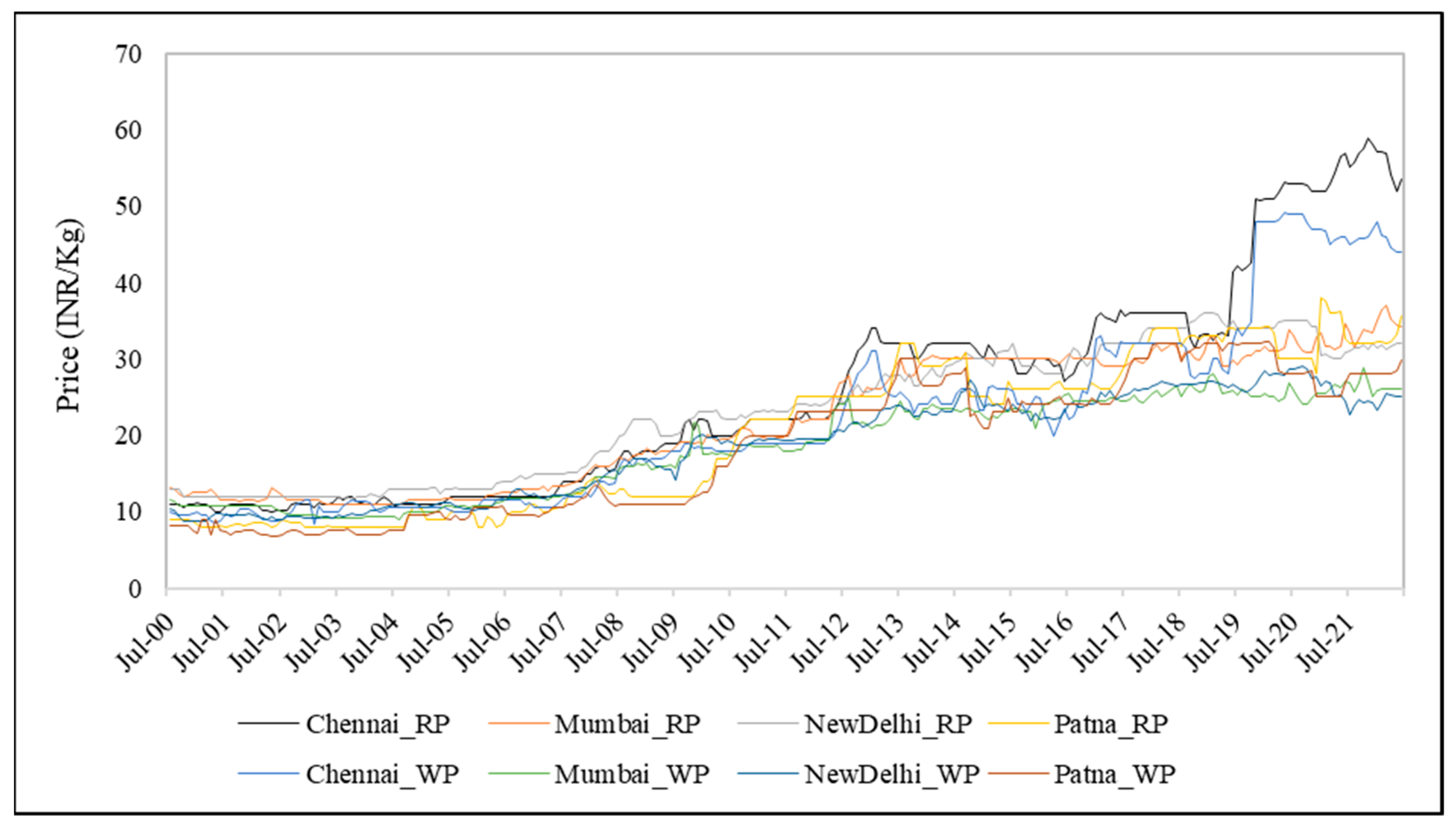
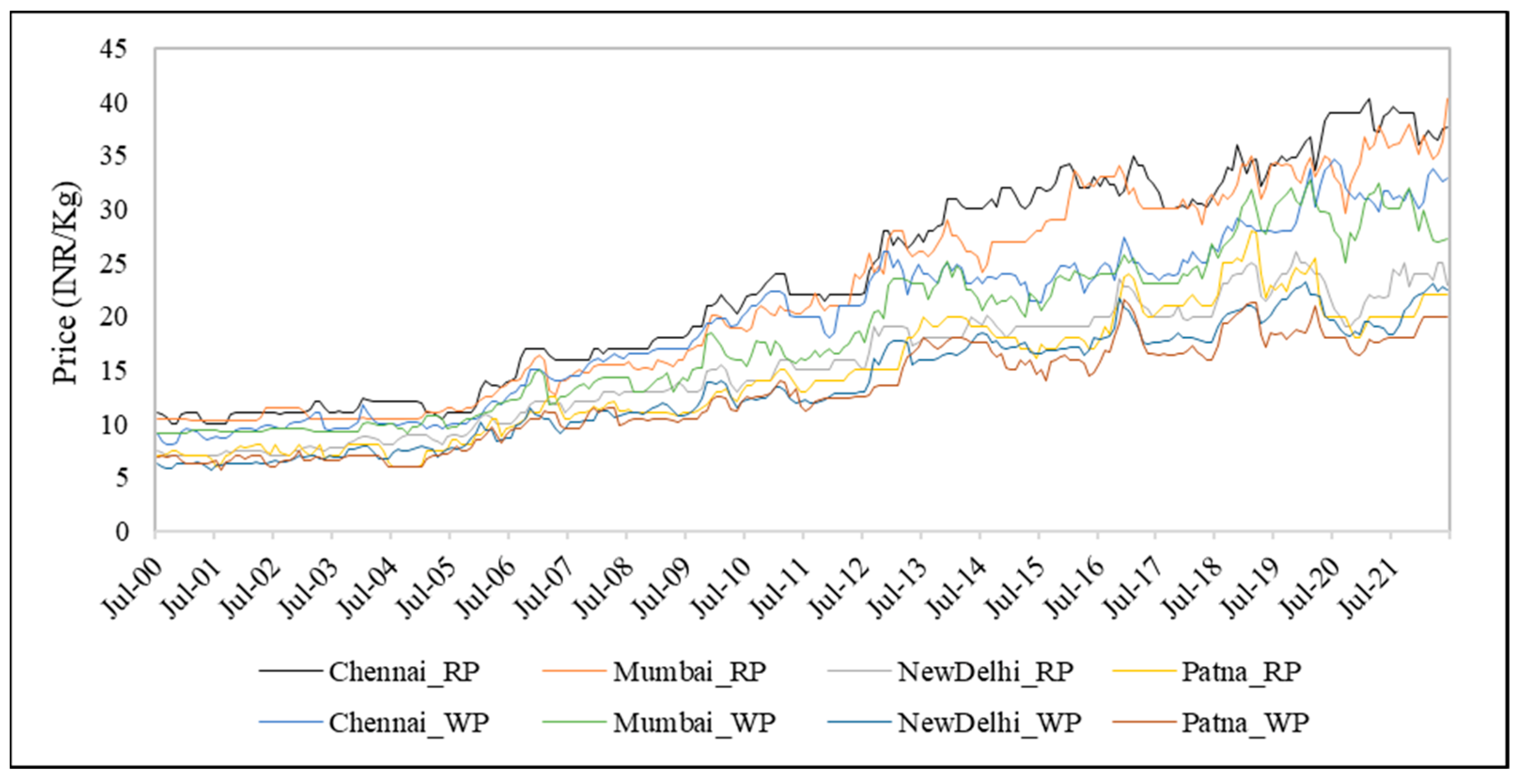
India was purposively selected, being one of the largest producers and consumers of rice and wheat. The study was marshaled on the wholesale and retail monthly prices of rice and wheat for four selected markets in India viz. Chennai (South), Delhi (North), Mumbai (East), and Patna (West), covering four major regions (one representative market from each zone). The price data in ₹ per Kg (₹ refers to the Indian Rupee, the national currency, also denoted as INR) were compiled from the Food Price Monitoring and Analysis (FPMA) (https://fpma.fao.org/giews/fpmat4/#/dashboard/tool/domestic, accessed on 2 October 2022) tool of the United Nations Food and Agriculture Organization (FAO) for the agricultural year spanning from July 2000 to June 2022. Along with descriptive statistics, various analytical tools and techniques (analyzed using Excel, SPSS ver. 26, and EVIEWS ver. 13 software) were used for better interpretation of the research findings and to draw some valid conclusions.

2.1. Theoretical Framework

Deciphering the fluctuations in the prices of agricultural commodities across spatially separated markets helps us to understand the dynamic behavior of the time series across regions, which facilitates sketching out the economic implications [14,16,20]. In general, agricultural commodity prices tend to be noisy, non-stationary, and largely leptokurtic, posing challenges in capturing the dynamics. To start with, analyzing the growth in wholesale and retail markets’ price series helps to capture the spatial dynamics. Similarly, estimating the instability in prices gives a clue about the extent of risk involved [13,16]. It is expected that price series showing a higher growth has high risk due to the discernible change in the prices from the base period to the recent period. 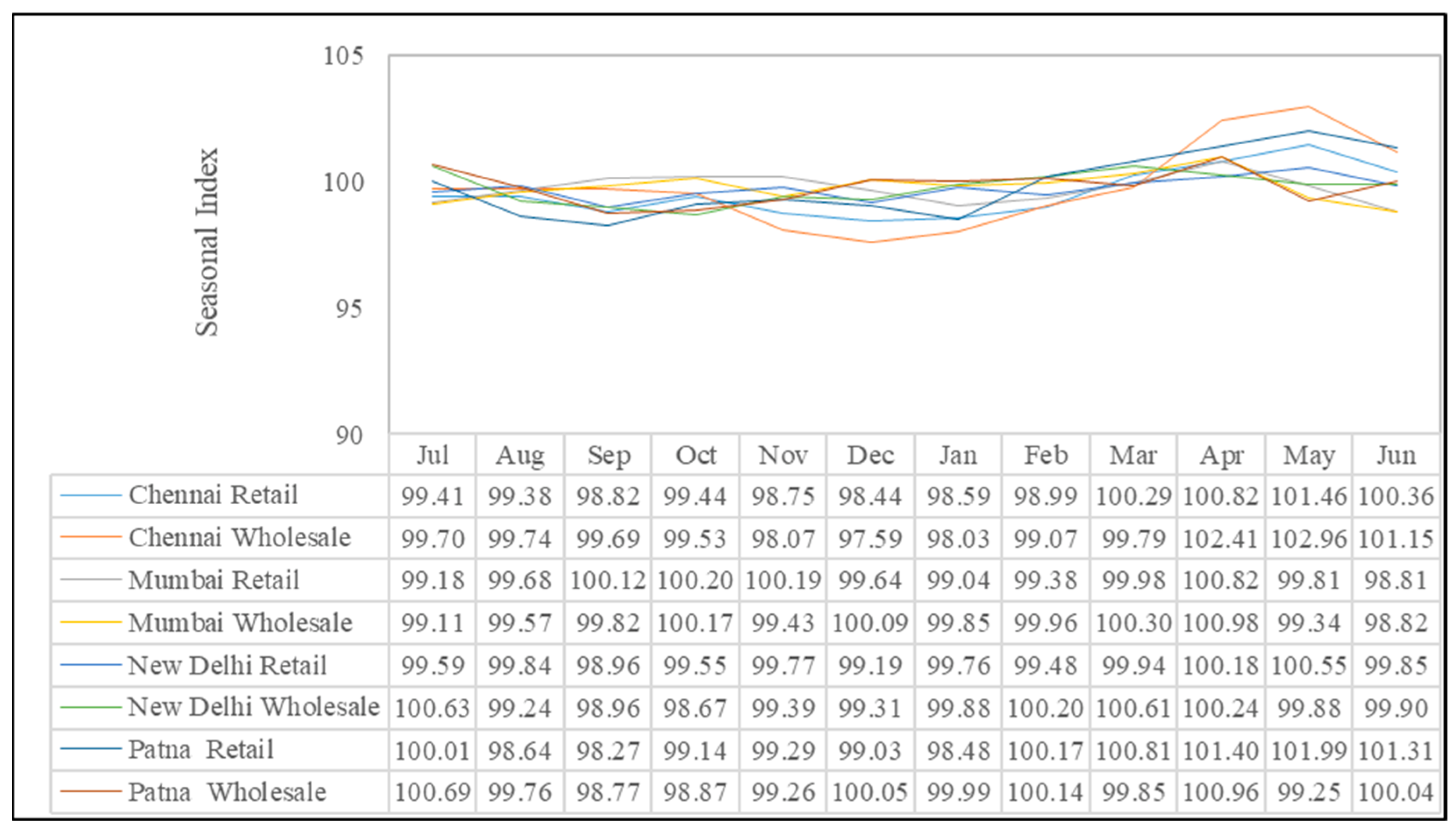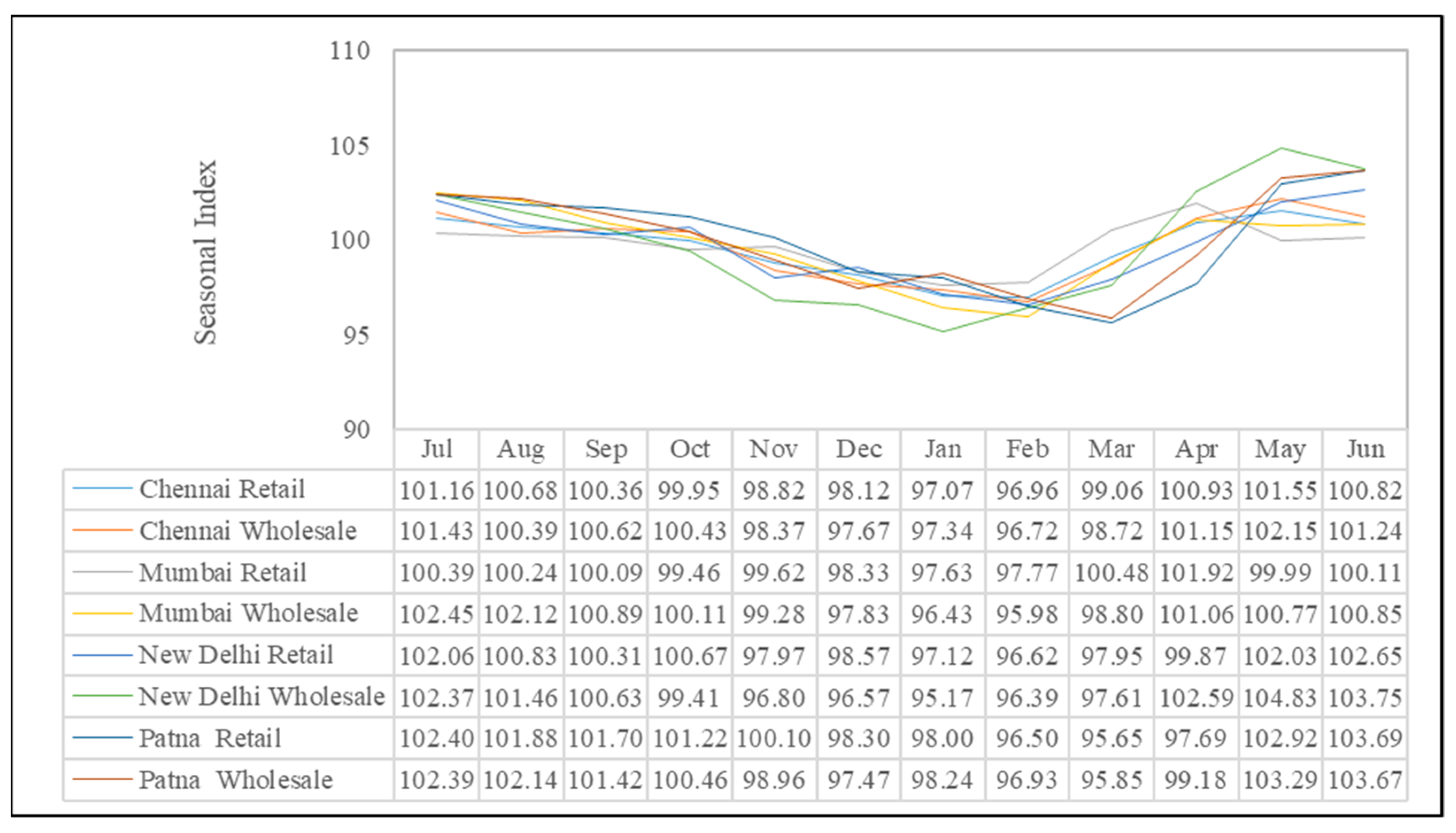In the next stage, estimating the variation in prices offers additional information on the behavior of the prices across markets, which guides policy makers to devise appropriate decisions [13,16]. As agricultural commodities production is seasonal in nature, price deseasonalization has to be undertaken to capture the actual variation [16,20]. Comparing the seasonal indices across the different markets would enhance our understanding of the price variation as the commodity is produced at some period of the year, but consumption takes place throughout the year. Intra-year price rises and average seasonal price variations are some indicators in price dynamics analysis that evaluate the degree of seasonal price variation.

To model the price series for analyzing the extent of integration between two or more markets, cointegration analysis attains significance. However, considering the longer period of the data, there exists the possibility of structural breaks in the price series, and these have to be detected to produce reliable results. Literature contains a vast amount of work on the issues related to structural change, the majority of it specifically designed for the case of a single period, but macroeconomic parameters generally have more than one structural break and most researchers have shown interest in knowing the basic procedure to structural breaks. As far as the significant literature is concerned, Quandt [34], Brown et al. [35], Ploberger et al. [36], Andrews [37], and Hansen [38] have contributed to testing the problem of structural breaks. Structural breaks can be divided into two types—i.e., known structural breaks like the 2008 financial crisis or the COVID-19 pandemic, and unknown structural breaks. When the structural break is known, the Chow test is more appropriate. However, in the case of unknown structural breaks, no prior understanding of the structural change that manifested itself in its time, nature, and shift is needed.

Bai and Perron [39] provided a comprehensive analysis of several issues regarding multiple structural change models, and developed some tests. These tests are helpful to capture the present change(s) and also determine, endogenously, the points of break with no prior knowledge. Under this approach, first, the structural breaks are detected using the time-series properties for all series in a system mode. Later, the price series are subjected to the stationarity test by determining whether they are trend stationary or difference stationary using the augmented Dickey–Fuller test [40,41]. This approach is effective in managing small samples and, if augmented sufficiently, it avoids uncertainty about variable exogeneity. After testing for stationarity, price series are subject to the cointegration test.

Price cointegration is an ideal situation wherein the prevailing prices of a commodity across locations follow a similar pattern in the long run [42,43]. Rapsomanikis et al. [44] discussed applying price cointegration tools, particularly for developing countries. A series of studies conducted on price cointegration suggested that market functionaries can achieve benefits through integrated markets [45,46,47,48]. Integrated markets encourage the dissemination of information across time, space, and form. Many studies have used the procedure introduced by Engle and Granger [49] to examine market integration. Thereafter, Johansen [50] introduced the alternative technique to examine price cointegration along with multiple cointegrating vectors. In this line, Kumar and Sharma [51] observed that Johansen’s test, having multiple advantages, is very easy to compute and robust enough with sans a priori assumptions on variables with testing, simultaneously, the number of cointegration vectors un-imposed earlier. After the cointegration analysis to assess the co-movement, a causality test is widely suggested. 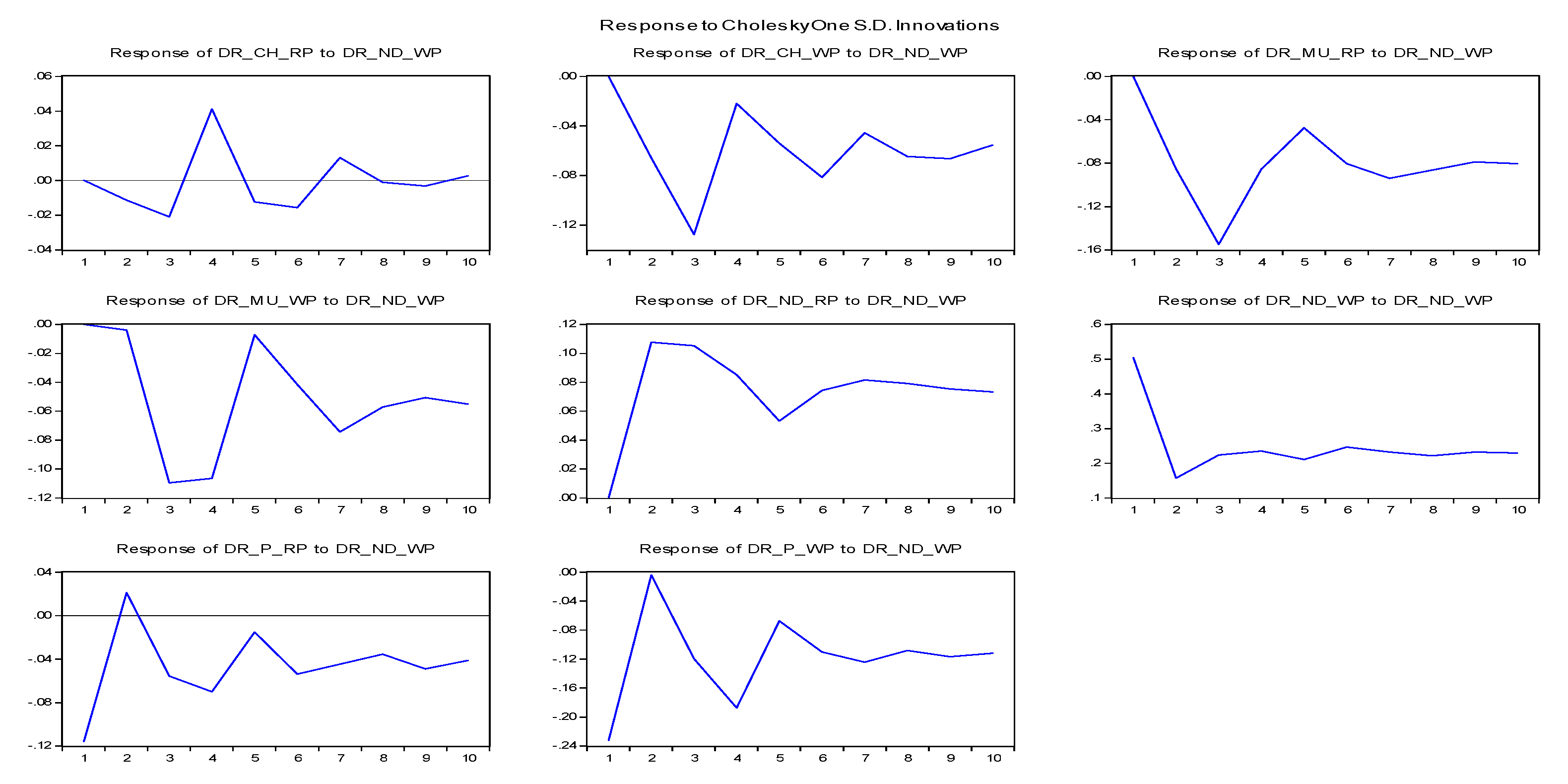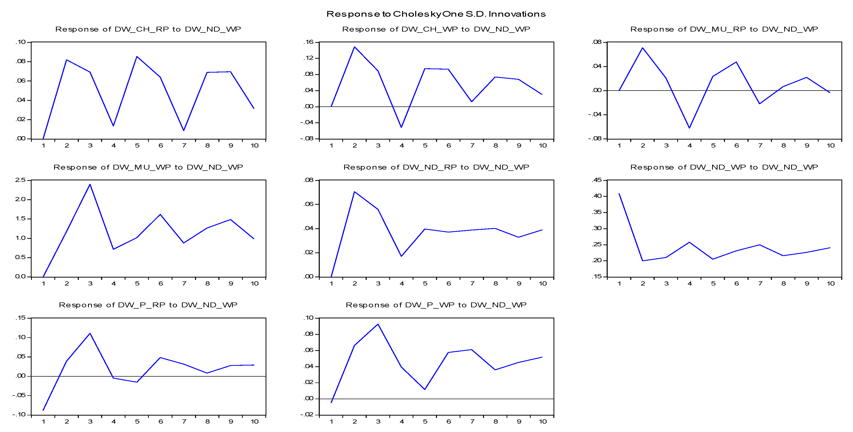So, after post-testing for cointegration using Johansen’s approach, Granger causality analysis [52] is undertaken to know the cause-and-effect relationship between the selected markets. The purpose of this statistical test is to determine whether a given price series (market A) and its lags explain the prediction of another series (market B). In addition, the current study has calculated impulse response [53,54] to obtain the dynamic interrelationships among the prices of different markets. The purpose is to investigate whether the mechanism of shocks, if any, persists in the market ecosystem. The analysis tracks the effect of ‘one’ SD (standard deviation) or ‘one’ unit shock imposed on one price series that is then reflected on the current and future values of all the endogenous variables over a specific time period [55]. Following the aforementioned theoretical framework, the detailed tools used in the study are given below.

2.2. Estimation of Growth Rate

The growth in wholesale and retail prices of both food commodities was calculated by using the below-mentioned formula [40,56,57]:

$$P_t=a_0{\left(1+b\right)}^t$$

The equation was transformed into logarithmic function before estimating the growth rate using the ordinary least squares method [40].

$$ln P_t=ln a_0+t ln\left(1+b\right)$$

where

P_t represents the price at time ‘t’,

$a$₀ denotes constant, and

b represents the growth rate.

2.3. Price Instability Index

The Cuddy-Della Valle Index (CDVI) approach was used to examine the magnitude of variation and risk involved in the prices of rice and wheat [58].

$$CDVI=CV\times \sqrt{\left(1-R^2\right)}$$

where

CDVI is the Cuddy-Della Valle instability Index (%),

CV is the Coefficient of Variation (%), and

$R^2$is the coefficient of multiple determination.

2.4. Seasonal Price Index

The seasonal index—measured using the 12-months ratio to the moving average method—is a way to measure the variations in prices across the commodity production seasons [59]. Subsequently, deseasonalization was carried out to eliminate seasonal variations in wholesale and retail prices of rice and wheat for the selected markets in India. The de-seasonalized commodity prices were calculated by adopting the given formula [59]:

$$\mathrm{Deseasonalized}\mathrm{data}=\frac{Actual Data for i^{th} month }{Seasonal index for i^{th} month}\times 100$$

In addition, the Intra-year Price Rise (IPR in %) and Average Seasonal Price Variation (ASPV in %) were estimated to evaluate the degree of seasonal price variations in rice and wheat for the selected markets in India.

$$IPR=\frac{SPIH-SPIL}{SPIL}\times 100$$

$$\mathrm{ASPV}=\frac{SPIH-SPIL}{\left(SPIH+SPIL\right)/2}\times 100$$

where

SPIH is the seasonal price index with the maximum value, and

SPIL is the seasonal price index with the minimum value.

2.5. Price Cointegration

Before applying any test, the foremost important step in the time series data is to check the stationarity and detect structural breaks, if any, since the considered time period is too long (July 2000 to June 2022). A stationary time series is one whose statistical properties like mean, variance, and covariance are invariant. The estimated relationship may be counterfeit without any significant implication in the absence of stationarity. The wholesale and retail price series of rice and wheat crops in the selected markets were first checked for stationarity by using the Augmented Dickey–Fuller (ADF) unit root test [40,41].

2.5.1. Detection of Multiple Unknown Structural Breaks

Of the two types of structural break, the study considers the detection of multiple unknown breaks following the below linear regression with ‘m’ breaks (m+1 regime):

$$y_t=\alpha +x_t \beta +z_t {\delta }_j+{\mu }_t t=T_{j-1} +1, \dots , T_j$$

where

𝑦_𝑡 is a function of 𝑋_𝑡 and 𝑍_𝑡; j = 1, …, m + 1; x_t (p × 1) and z_t (q × 1) are vectors of covariates; β and δ_j(j = 1, …, m + 1) are the corresponding vectors of coefficients; and u_t is the disturbance at time t. The assumption that underlying economic events remain constant across the entire period is relaxed in the structural breakpoint. Before presenting the results, it is important to know the hypotheses of this study.

H₀: 

There is structural stability.

H₁: 

There are structural breaks.

The p-values enable us to accept or reject the null hypothesis. The study of structural breaks is inevitable in macro-econometric modeling due to structural changes or regime shifts such as systemic shocks—e.g., price fluctuations, demand and supply shocks—and economic and institutional changes.

2.5.2. Unit Root Test

The Augmented Dickey–Fuller (ADF) test was carried out to examine the stationarity in the data [40,41]. The ADF test is executed by estimating the following equation:

$$\mathsf{\Delta }{P}_t={\alpha }_0+{\delta }_{1}t+{\beta }_1{P}_{t-1}+{{\displaystyle \sum }}_{j=1}^q{\beta }_1\mathsf{\Delta }{P}_{t-j}+{\epsilon }_t$$

where

$\mathsf{\Delta }{P}_t=P_t-P_{t-1},\mathsf{\Delta }{P}_{t-1}=P_{t-1}-P_{t-2},\dots \mathsf{\Delta }{P}_{n-1}=P_{n-1}-P_{n-2}$

P represents price,

${\alpha }_{0 }$is the constant,

t represents time,

q is the number of lag length, and

${\epsilon }_t$ is the random error-term.

Unit root testing was carried out by framing the null hypothesis, H₀: ${\beta }_1$= 0; that is, there is a unit root and the time series is non-stationary, and the alternative hypothesis, H₁:$\beta { }_1$< 0; that is, the time series is stationary. A rejection of the null hypothesis suggests that the particular price series is stationary [40].

2.5.3. Cointegration Test

To test the long-run relationship in commodity prices between the wholesale and retail markets, the study used the Johansen’s cointegration test [50,60]. The null hypothesis (H₀) of utmost ‘r’ cointegrating vectors—i.e., rank of error-correction coefficient matrix—against a general alternative hypothesis (H₁) of ‘r+1′ cointegrating vectors is tested by trace and maximum eigenvalue statistics [34].

$$J_{trace}=-T{\displaystyle \sum }_{i=r+1}^N\left(1-{\widehat{\lambda }}_1\right)$$

$${\lambda }_{max}=-T\left(1-{\widehat{\lambda }}_{r+1}\right)$$

where r is the number of cointegrated vector, ${\widehat{\lambda }}_1$ is the eigenvalue and ${\widehat{\lambda }}_{r+1}$ is the (r + 1)th largest squared eigenvalue obtained from the parameter matrix of the cointegrated system, and T is the effective number of observations.

In the present study, we have found that the wholesale and retail price series of rice and wheat crops have structural breaks. In order to see the effect of such breaks on the cointegration of the rice and wheat markets, we have introduced three dummies for each crop in our model. These breaks have been incorporated as the methodology given by Johansen et al. [61].

2.6. Granger Causality Test

The Granger causality test has been employed to know the path of price transmission across markets [52]. The Granger causality test is carried out for a market pair, testing whether price series P_t Granger-causes price series Q_t, and vice versa. All sorts of permutations and combinations are possible within the selected markets viz. univariate Granger causality indicating price transmission from P_t to Q_t or from Q_t to P_t, bivariate Granger causality depicting price transmission in both directions, or absence of causality implying no price transmission. The above test is carried out using the following equation:

$$P_t={\displaystyle \sum }_{i=1}^m{\alpha }_i{P}_{t-i}+{\displaystyle \sum }_{j=1}^m{\beta }_j{Q}_{t-j}+{\epsilon }_{1\mathrm{t}}$$

$$Q_t={\displaystyle \sum }_{i=1}^m{\alpha }_i{Q}_{t-i}+{\displaystyle \sum }_{j=1}^m{\beta }_j{P}_{t-j}+{\epsilon }_{2\mathrm{t}}$$

where

P and Q are the selected market prices series pair,

and

t indicates the time period.

The subscripts, ‘i’ and ‘j’ represent the number of lags pertaining to the respective price series.

The null hypothesis states that ln P_t does not Granger-cause ln Q_t, and its rejection implies that there is Granger causality between the selected price series pair [40].

2.7. Impulse Response Function

In the present study, the Generalized Impulse Response Function (GIRF) proposed by Koop et al. [53] and further advocated by Pesaran and Shin [54] has been employed. The GIRF of a random current shock ‘$\delta$’ and historical shock ‘$w_{t-1}$’ is given in the below equation:

$$GIRF Y \left(h, \delta , w_{t-1}\right)=E\left[Y_t+h|\delta , w_{t-1}\right]-E\left[y_t+h|w_{t-1}\right]\mathrm{for}\mathrm{t}=0,1,2\text{…}\mathrm{n}$$

(1)

3. Results and Discussion

3.1. Price Dynamics in Rice and Wheat Markets

Figure 1 shows the sharp fluctuations in the monthly price for selected rice markets. It is apparent that the commodity prices have been increasing during the study period, i.e., from 2000–01 to 2021–22, regardless of market type and region. Both the rice and wheat prices show an upward trend, but a higher fluctuation is observed in wheat prices (Figure 2). Further, a common movement is observed in the prices of wheat and rice but it differs in magnitude. A recurrent problem of Indian agriculture is the boom-and-bust cycle in commodity prices along with a geographical concentration in production. Accordingly, the rice and wheat market prices (

Table 1. Summary statistics for the rice and wheat prices (July 2000 to June 2022).

Particulars	Chennai		Mumbai		New Delhi		Patna
	Retail	Wholesale	Retail	Wholesale	Retail	Wholesale	Retail	Wholesale
Rice
Mean (₹/Kg)	25.5	22.0	21.9	18.3	23.0	18.5	20.2	18.6
Min (₹/Kg)	10.0	8.4	11.0	9.0	11.5	8.8	8.0	6.8
Max (₹/Kg)	59.0	49.1	37.0	28.9	36.0	29.1	38.0	32.3
SD (₹/Kg)	14.0	11.8	8.5	6.4	8.4	6.7	9.9	8.9
CV (%)	139.7	141.0	77.2	70.6	72.8	76.0	124.9	132.5
CDVI (%)	16.1	20.0	6.0	5.7	5.0	5.8	12.4	16.5
CAGR (%)	0.7	0.7	0.5	0.5	0.5	0.5	0.7	0.7
Skewness	0.8	0.9	0.0	−0.2	−0.1	−0.2	0.0	0.0
Kurtosis	−0.3	−0.2	−1.7	−1.6	−1.5	−1.5	−1.6	−1.6
Wheat
Mean (₹/Kg)	23.3	19.7	21.8	18.3	15.4	13.6	14.5	12.8
Min (₹/Kg)	10.0	8.0	10.3	9.0	7.0	5.7	6.0	5.7
Max (₹/Kg)	40.3	34.7	40.4	32.7	26.0	23.2	28.0	21.6
SD (₹/Kg)	9.7	7.6	9.2	7.3	5.7	5.2	5.8	4.7
CV (%)	97.3	94.9	89.5	81.2	81.3	90.6	96.6	81.6
CDVI (%)	3.9	4.4	4.0	4.9	3.6	4.7	10.3	7.4
CAGR (%)	0.6	0.5	0.6	0.5	0.5	0.5	0.5	0.5
Skewness	0.1	0.0	0.1	0.3	0.0	0.1	0.2	0.0
Kurtosis	−1.5	−1.2	−1.5	−1.2	−1.3	−1.3	−1.2	−1.3

) revealed a substantial variation, both spatially and temporally [2,13,62]. Further, the price deviation between the wholesale and retail markets witnessed a considerable increase during the study period (Figure 2), signifying the necessity to investigate the extent of price cointegration and direction of price transmission for these two agricultural commodities.

The growth, variation, and summary statistics pertaining to major regional rice and wheat market prices showed a distinct pattern and behavior that existed between the wholesale and retail prices (Table 1). Among the regional markets, Patna registered the lowest estimated values for a majority of the price behavior indicators with respect to both rice and wheat. In the case of wheat, Chennai witnessed the highest wholesale (₹23.30 kg⁻¹) and retail (₹19.70 kg⁻¹) prices. The possible reason is, inter alia, ‘nil’ production in and around the Chennai region, in spite of escalating demand for wheat and wheat-based food products, especially originating from the urban class owing to the increase in the income levels [57]. In the case of rice, the deviation between the wholesale and retail prices was highest in Delhi (₹4.50 kg⁻¹), followed by Mumbai (₹3.60 kg⁻¹), Chennai (₹3.50 kg⁻¹), and Patna (₹1.60 kg⁻¹). Likewise, the price divergence between wholesale and retail markets was highest in Chennai (₹3.60 kg⁻¹) with respect to wheat, followed by Mumbai (₹3.50 kg⁻¹), Delhi (₹1.80 kg⁻¹), and Patna (₹1.70 kg⁻¹). For both the staple food commodities, the wholesale and retail prices were lowest in the case of Patna, indicating a region with abundant supply owing to substantial production in comparison to others. Inter alia, the quantum jumps in these commodities in the recent past, i.e., between 2000–01 and 2017–18, led to increased supply and subsequently a decline in the wholesale prices, especially in rice [43], a proxy variable considered as a producer/farmer/farm-gate price [2].

Skewness estimates indicated positive values ranging between 0 and 0.90 for rice, and between 0 and 0.30 in the case of wheat. The positively skewed values explicitly indicate that the price series distribution is stretched over the right tail against the left, corroborating the findings of past research [63]. In contrast, the estimates of kurtosis were negative for all the price series pertaining to rice and wheat markets, implying the flat/short-tailed (platykurtic) distribution, i.e., comparatively, a flat distribution in relation to normal distribution; however, a wide peak exists [46].

The estimates of standard deviation (SD) and CV were highest in the case of Chennai for both types of cereals, i.e., rice and wheat, as well as for market types, i.e., wholesale and retail (Table 1). The possible reason for this is that Chennai from the southern zone of India is a region wherein the production capacity is low, especially for wheat. Hence, it has to depend on other production regions to manage the increasing consumption demand, leading to higher SD and variation. On the contrary, Delhi witnessed the lowest values as the capital region with a higher rate of consumption. In recent research [14], the CV was found to be consistent for all wholesale and retail wheat markets in India. The CDVI, an indicator of price risk and instability, shows that, with the exception of the Delhi and Mumbai regions, the rest had more than 15 per cent in the case of rice. On the contrary, in the case of wheat, barring the wholesale and retail prices in Patna, the rest of the regions had CDVI less than five per cent. The analysis of price growth using the Compound Annual Growth Rate (CAGR) indicated a positive trend and it was less than one per cent per month. In the case of rice and wheat, the price growth was highest in Chennai. The possible reason for wheat is ‘nil’ production in and around the Chennai region.

3.2. Seasonal Variation in the Prices of Rice and Wheat

Generally, the seasonal variations in agricultural food commodities occur regularly and this has to be monitored systematically for planning and taking agri-business decisions. An analysis of seasonal variation in rice and wheat prices showed a distinct pattern (Figure 3 and Figure 4). In the case of rice, the seasonal price index (Figure 3) was highest and lowest in the Chennai wholesale market, respectively, during May (102.96) and December (97.59). The estimated index values were higher during March and April, i.e., before the crop harvest, wherein the rice supply is low resulting in higher indices. Our findings contradict the results of Kumare et al. [16]. Subsequently, the index values witnessed a fall due to the increase in market arrivals post-harvest [19,20]. Among the regions, seasonal price variation was relatively more in Patna and less in Chennai, indicating the spatial dynamics. Among the months, it was higher during April to May for about three markets and it was lower during August for three markets with the exception of Delhi and Patna. Less variation is attributed to the market arrivals linked to crop harvest and/or release of public stock by the Government [20] to meet public demand.

It is also interesting to compare the price variations of wheat across different markets in India. The seasonal index for wheat was highest in the Delhi wholesale market (May: 104.83), and it also registered the lowest (December: 95.17). Overall, Delhi witnessed the higher seasonal price variation, whereas Mumbai experienced the lower indices in comparison to other regions. The price indices for wheat were highest in the month of May for about three markets under study, barring the wholesale + retail markets in Mumbai and Patna. On the contrary, they were lowest in the month of July for about three markets. In general, January and February registered lower values owing to increased supply and/or public stock release [19,20].

On perusal of

Table 2. Average de-seasonalized monthly prices of rice and wheat (July 2000 to June 2022).

Particulars	Chennai		Mumbai		New Delhi		Patna
	Retail	Wholesale	Retail	Wholesale	Retail	Wholesale	Retail	Wholesale
Rice
July	24.73	21.35	21.76	18.39	22.79	18.01	19.66	17.99
August	24.85	21.38	21.60	18.26	22.76	18.53	20.29	18.43
September	25.20	21.46	21.43	18.16	23.23	18.65	20.61	18.93
October	25.04	21.57	21.45	18.08	23.01	18.79	20.21	18.79
November	25.80	22.62	21.54	18.40	22.94	18.59	20.16	18.67
December	26.08	22.96	21.91	18.19	23.32	18.71	20.27	18.37
January	26.22	23.11	22.35	18.33	23.06	18.50	20.87	18.46
February	26.19	22.85	22.33	18.38	23.31	18.57	20.41	18.51
March	25.70	22.43	22.11	18.31	23.12	18.54	20.13	18.66
April	25.49	21.48	21.72	18.14	23.15	18.66	19.95	18.38
May	25.36	21.37	22.18	18.80	23.08	18.74	20.02	19.03
June	26.20	22.26	22.85	19.12	23.45	18.83	20.44	19.08
Wheat
July	22.22	18.61	21.00	17.02	14.42	12.57	13.59	11.97
August	22.54	19.11	21.19	17.24	14.82	12.85	13.84	12.13
September	22.74	19.05	21.33	17.74	15.03	13.13	13.87	12.28
October	22.95	19.15	21.72	18.16	14.94	13.48	14.08	12.55
November	23.65	20.03	21.74	18.45	15.88	14.33	14.44	12.97
December	24.01	20.50	22.43	19.09	15.68	14.42	14.98	13.40
January	24.49	20.59	22.89	19.71	16.18	14.89	15.23	13.33
February	24.75	21.07	22.96	19.99	16.43	14.59	15.75	13.73
March	23.67	20.27	21.82	18.89	16.03	14.32	15.99	14.04
April	22.97	19.40	21.29	18.09	15.59	13.13	15.22	13.10
May	22.98	19.25	22.19	18.24	15.05	12.62	13.89	12.22
June	23.48	19.71	22.42	18.34	14.82	12.92	13.80	12.20

, it is explicit that the average de-seasonalized price observations between 2000–01 and 2021–22 in the case of wholesale prices for both rice and wheat were lower to their counterpart, as expected. The deviation between wholesale prices and retail prices for rice was relatively higher in New Delhi, followed by Mumbai and Chennai (Table 2). Further, the average de-seasonalized price values pertaining to wheat were found to be of the same level in terms of magnitude in the corresponding markets.

The indices were highest in Chennai, followed by Mumbai and Delhi. The divergence between wholesale prices and retail prices for wheat was relatively higher in the period of May to June, coinciding with post-harvest. A comparative analysis between price indices and de-seasonalized prices provides implications for multi stakeholders in the rice and wheat value chain—namely, producers/farmers, traders, millers/processors, and consumers who can use the vital information for taking rational agri-business decisions like production, purchase, marketing, processing, stocking, distributing, and consumption [20].

Across the rice markets, the CAGR in seasonal indices was found to be negative except for Mumbai’s retail price, and the declining growth was less than ‘one’ per cent (

Table 3. Growth and variation in seasonal price index of rice and wheat.

Market	Prices	CV (%) a	CAGR (%) b	IPR (%) c	ASPV (%) d
Rice
Chennai	Retail	0.97	−0.09	3.07	3.02
	Wholesale	1.66	−0.14	5.50	5.36
Mumbai	Retail	0.57	0.04	2.04	2.02
	Wholesale	0.58	−0.03	2.18	2.15
New Delhi	Retail	0.42	−0.05	1.61	1.59
	Wholesale	0.63	−0.12	2.00	1.98
Patna	Retail	1.26	−0.14	3.79	3.72
	Wholesale	0.67	−0.08	2.21	2.19
Wheat
Chennai	Retail	1.60	0.11	4.74	4.63
	Wholesale	1.83	0.08	5.62	5.46
Mumbai	Retail	1.24	0.03	4.40	4.31
	Wholesale	2.10	0.21	6.74	6.52
New Delhi	Retail	2.05	0.16	6.24	6.05
	Wholesale	3.26	0.04	10.15	9.66
Patna	Retail	2.68	0.32	8.41	8.07
	Wholesale	2.61	0.17	8.16	7.84

^a Coefficient of Variation, ^b Compound Annual Growth Rate, ^c Intra-year Price Rise, and ^d Average Seasonal Price Variation.

). The CV for seasonal indices hovered around ‘one’ per cent, and it ranged from 0.42 to 1.66 per cent, respectively, for the Mumbai retail market and the Chennai wholesale market. The IPR and ASPV for rice were highest in the Chennai wholesale market and lowest in the case of the Mumbai retail market (Table 3). The IPR with respect to rice ranged from 1.61 to 5.50 per cent, while the ASPV ranged from 1.59 to 5.36 per cent.

In the case of wheat, the estimated growth in seasonal indices was positive but less than ‘one’ per cent in all regions. The variation in seasonal indices hovered around ‘two’ per cent (Table 3) and it ranged from 1.24 to 3.26 per cent, respectively, for the Chennai retail market and the Delhi wholesale market. The IPR and ASPV for the wheat market were found to be highest in the New Delhi wholesale market and lowest in the Mumbai retail market (Table 3). The IPR for wheat ranged from 4.40 to 10.15 per cent, while the ASPV ranged from 4.31 to 9.66 per cent. The estimates of IPR and ASPV also provide vital inferences for taking agri-business-oriented decisions. Finally, the extent of fluctuations in seasonal index values of wheat and rice was computed through the ASPV as indicated in Table 3 [19].

3.3. Structural Breaks in Rice and Wheat Prices

The results of structural break analysis (

Table 4. Structural breaks for wheat and rice price series.

Commodity	Structural Breaks
Rice	2019M04
	2013M03
	2009M04
Wheat	2013M12
	2019M04
	2006M01

) revealed that, in the case of rice crop, the first structural break (as a price system) occurred during April 2009. Subsequent structural breaks were observed during the 2013 (March) and 2019 (April). During this period, the major break occurred in 2019 (April). In the case of rice, the months of structural breaks coincided with the highest seasonal index values, wherein the supply was low owing to the pre-harvest period (refer to Figure 3).

In the case of wheat crop, the first structural break was observed during 2006 (January). The next two structural breaks were observed during 2013 (December) and 2019 (April), coinciding with the post-sowing and pre-harvest periods. It is surprising to note that the structural break did not coincide with the expected 2008 financial crisis or the recent-past COVID-19 pandemic. This indirectly implies that the Government intervention in these staples at regular intervals through price policies safeguarded the food sector from unwarranted fluctuations [33] and social unrest.

3.4. Price Cointegration in Rice and Wheat Markets

The hypothesis under efficient markets is the perfect integration of commodity prices, which should adjust and correct instantly with the available information [63]. The ADF test indicated the presence of unit root in all the level series, followed by stationarity in their first differencing (

Table 5. Estimates of unit root test for the monthly prices of rice and wheat markets with structural break.

Market	Prices	Level (Assumption: Constant, Linear Trend)		First Difference (Assumption: Constant)
		ADF Statistic	p-Value	ADF Statistic	p-Value
Rice
Chennai	Retail	−1.861	≥0.10	−14.382 *	<0.01
	Wholesale	−1.948	≥0.10	−14.320 *	<0.01
Mumbai	Retail	0.098	≥0.50	−15.378 *	<0.01
	Wholesale	−0.042	≥0.50	−15.727 *	<0.01
New Delhi	Retail	0.467	≥0.50	−15.104 *	<0.01
	Wholesale	−0.200	≥0.50	−15.280 *	<0.01
Patna	Retail	−0.447	≥0.50	−15.824 *	<0.01
	Wholesale	−0.100	≥0.50	−15.125 *	<0.01
Wheat
Chennai	Retail	−0.197	≥0.50	−13.348 *	<0.01
	Wholesale	−0.544	≥0.50	−13.288 *	<0.01
Mumbai	Retail	−0.058	≥0.50	−10.384 *	<0.01
	Wholesale	−0.724	≥0.50	−15.949 *	<0.01
New Delhi	Retail	−1.320	≥0.50	−14.339 *	<0.01
	Wholesale	−1.394	≥0.50	−13.204 *	<0.01
Patna	Retail	−0.957	≥0.50	−12.094 *	<0.01
	Wholesale	−1.379	≥0.50	−13.379 *	<0.01

Note: For rice, the structural break is considered to be 2019M04; For wheat, the structural break is considered to be 2013M12; * indicates the significance at the five per cent level of MacKinnon’s (1996) one-sided probability value.

). The original series of wholesale and retail price for both rice and wheat was non-stationary and non-significant, but the first-order differenced series turned out to be stationary and is significant at the five per cent level. Similar results were obtained in several market integration studies [14,19,20,22]. It was concluded from the ADF test that the variables were integrated of order one [I (1)]. It is thus inferred that, in all the cases, price shocks (and crashes) have a long-lasting outcome on the price levels in the upcoming period [17]. The confirmation that each level series is I (1) helped to proceed with Johansen’s cointegration analysis [2,14,17] for capturing the price signal transmissions [17].

The correlation coefficient of wholesale and retail prices for rice and wheat in different market pairs was calculated to determine the degree of market association. Prior to performing the cointegration analysis, the correlation after removing the cross-correlation between market prices was investigated. The results reported in

Table 6. Estimates of the correlation for rice markets.

Price	Markets	Chennai	Mumbai	New Delhi	Patna	Chennai	Mumbai	New Delhi	Patna
		Retail				Wholesale
Retail	Chennai		0.13 *	0.09	0.00	0.74 **	−0.04	0.13 *	−0.03
	Mumbai	0.13 *		0.04	0.06	0.10	0.57 **	0.06	0.08
	New Delhi	0.09	0.04		−0.25	0.04	0.04	0.35 **	0.01
	Patna	0.00	0.06	−0.25 **		−0.02	0.06	−0.16 *	0.55 **
Wholesale	Chennai	0.74 **	0.10	0.04	−0.02		−0.04	0.11	−0.04
	Mumbai	−0.04	0.57 **	0.04	0.06	−0.04		0.10	0.11
	New Delhi	0.13 *	0.06	0.35 **	−0.16 *	0.11	0.10		−0.14 *
	Patna	−0.03	0.08	0.01	0.55 **	−0.04	0.11	−0.14 *

** and * indicate the significance of correlation coefficient respectively at the one and five per cent level of probability (2-tailed), respectively.

and

Table 7. Estimates of the correlation for wheat markets.

Price	Markets	Chennai	Mumbai	New Delhi	Patna	Chennai	Mumbai	New Delhi	Patna
		Retail				Wholesale
Retail	Chennai		0.19 **	0.20 **	0.03	0.46 **	0.22 **	0.12	0.06
	Mumbai	0.19 **		0.08	0.01	0.22 **	0.67 **	0.10	−0.01
	New Delhi	0.20 **	0.08		0.32 **	0.03	0.22 **	0.61 **	0.33 **
	Patna	0.03	0.01	0.32 **		0.02	0.18 **	0.24 **	0.80 **
Wholesale	Chennai	0.46 **	0.22 **	0.03	0.02		0.20 **	0.15 *	0.07
	Mumbai	0.22 **	0.67 **	0.22 **	0.18 **	0.20 **		0.18 **	0.14 *
	New Delhi	0.12	0.10	0.61 **	0.24 **	0.15 *	0.18 **		0.29 **
	Patna	0.06	−0.01	0.33 **	0.80 **	0.07	0.14 *	0.29 **

** and * indicate the significance of correlation coefficient respectively at the one and five per cent level of probability (2-tailed), respectively.

show the degree of short-run linear association as revealed by the correlation coefficients after the removal of serial dependance. The results of correlation analysis revealed that the wholesale and retail prices of respective markets are highly correlated with each other, in linear terms. Kumare et al. [16] analyzed the price correlation between two regional rice markets in Maharashtra and found a strong and positive degree of price association. In our study, the correlation coefficient was found to be positive and significant for Patna, New Delhi, Mumbai, and Chennai with a value of 0.55, 0.35, 0.57, and 0.74, respectively, owing to the symmetric price movement in those markets (Table 5). The value of the correlation coefficient between two market pairs of wheat—i.e., Chennai–Delhi, Patna–Chennai, Patna–Mumbai, and Mumbai–Delhi—was found positive and significant. The implication is that the retail and wholesale prices of wheat were interlinked in all the selected markets—i.e., if the price increases in one market it leads to an increase in the price prevailing in the other market (Table 6). In addition, Pearson’s correlation was also estimated for rice and wheat markets following the structural breaks, as per Table 4, to capture any change in the correlation pattern. The correlation under structural breaks (refer to Supplementary Tables S1 and S2) did not depict any discernible change between periods following the structural breaks, with the exception of a few markets like Patna in the case of rice. However, the magnitude of correlation coefficients was higher during the period following structural break 2 with respect to rice. In wheat, a distinct pattern was noticed in the period following structural break 3. A majority of market pairs exhibited a negative correlation, indicating the price divergence between the retail and wholesale markets. The possible reason for the disconnect in price association can be attributed to the reflection that different parts of the economy are seeing a revival at different paces (https://rbidocs.rbi.org.in/rdocs/Publications/Pdfs/6241.pdf, accessed on 15 February 2023).

It is necessary to determine the optimum lag length (that measures the exact number of lag periods along the autoregressive process in order to test for the presence of any serial correlation) before cointegration analysis since Johansen’s cointegration is much more sensitive to the number of lags [64]. The optimum lag length was identified as ‘five’ and ‘four’ for rice and wheat, respectively, using the Akaike Information Criterion (AIC). The results, based on trace test and eigenvalue, show that the long-run cointegration was established and confirmed the price cointegration in the rice and wheat markets (

Table 8. Estimates of Johansen’s cointegration analysis of rice markets under structural break (Assumption: Linear deterministic trend).

No. of Cointegrating Equations	Eigenvalue	Trace Test Statistic	Critical Value	Probability Value **
Markets: Chennai, Mumbai, Delhi and Patna (Wholesale and Retail)
None (r = 0) *	0.3009	392.6260	285.1425	0.0000
At most 1 (r ≤ 1) *	0.2764	299.9188	239.2354	0.0000
At most 2 (r ≤ 2) *	0.1854	216.1112	197.3709	0.0041
At most 3 (r ≤ 3) *	0.1386	162.9917	159.5297	0.0319
At most 4 (r ≤ 4) *	0.1327	124.3565	125.6154	0.0595
At most 5 (r ≤ 5)	0.1127	87.4947	95.7537	0.1615
At most 6 (r ≤ 6)	0.0886	56.5257	69.8189	0.3571
At most 7 (r ≤ 7)	0.0595	32.4876	47.8561	0.5852
At most 8 (r ≤ 8)	0.0373	16.6015	29.7971	0.6693
At most 9 (r ≤ 9)	0.0232	6.7557	15.4947	0.6062
At most 10 (r ≤ 10)	0.0026	0.6807	3.8415	0.4093

Trace test indicates ‘five’ cointegrating equations at the five per cent level; * denotes rejection of the hypothesis at the five per cent level; ** MacKinnon–Haug–Michelis (1999) probability values.

and

Table 9. Estimates of Johansen’s cointegration analysis of wheat markets under structural break (Assumption: Linear deterministic trend).

No. of Cointegrating Equations	Eigenvalue	Trace Test Statistic	Critical Value	Probability Value **
Markets: Chennai, Mumbai, Delhi and Patna (Wholesale and Retail)
None (r = 0) *	0.2851	377.2649	285.1425	0.0000
At most 1 (r ≤ 1) *	0.2333	290.3574	239.2354	0.0000
At most 2 (r ≤ 2) *	0.1758	221.5681	197.3709	0.0017
At most 3 (r ≤ 3) *	0.1555	171.4772	159.5297	0.0094
At most 4 (r ≤ 4)	0.1474	127.7174	125.6154	0.0370
At most 5 (r ≤ 5)	0.1198	86.4277	95.7537	0.1842
At most 6 (r ≤ 6)	0.0875	53.3783	69.8189	0.4886
At most 7 (r ≤ 7)	0.0638	29.6693	47.8561	0.7357
At most 8 (r ≤ 8)	0.0298	12.5929	29.7971	0.9093
At most 9 (r ≤ 9)	0.0182	4.7671	15.4947	0.8330
At most 10 (r ≤ 10)	0.0000	0.0050	3.8415	0.9425

Trace test indicates ‘four’ cointegrating equations at five per cent level; * denotes rejection of the hypothesis at five per cent level; ** MacKinnon–Haug–Michelis (1999) probability values.

).

Overall, the cointegration test following the structural breaks (traced by considering eight price series and three structural breaks pertaining to a particular commodity—i.e., four wholesale price series, four retail price series, and three dummies on structural breaks) rejected the null hypothesis of no cointegration (r = 0) between the retail and wholesale prices at the five per cent probability level indicating the presence of five and four cointegration vectors (Table 9 and

Table 10. Price transmission between the rice markets by Granger causality test.

Price	Markets	Retail Price				Wholesale Price
		Chennai	Mumbai	New Delhi	Patna	Chennai	Mumbai	New Delhi	Patna
Retail	Chennai		×	×	×	×	×	×	×
	Mumbai	×		×	×	×	×	→	×
	New Delhi	×	×		×	×	×	↔	×
	Patna	×	×	×		×	×	→	×
Wholesale	Chennai	×	×	×	×		×	×	×
	Mumbai	×	×	×	×	×		→	×
	New Delhi	×	→	↔	×	→	→		×
	Patna	×	×	→	×	×	×	×

×: No Causality; →: Uni-directional; ↔: Bi-directional.

) among the retail and wholesale wheat and rice markets, respectively [2,50]. The implication is that the wheat and rice prices are strongly cointegrated in the long run. Mukim et al. [21] analyzed the extent of spatial market integration in Indian wheat and confirmed that the markets are integrated in the long run, but dis-integrated in the short run. Recent research [17] indicates that the extent of market integration is influenced by the choice of rice variety. Despite the presence of short-run linear association and long-run integration as evidenced by cointegration analysis, past research [20] identified that Chennai failed to exhibit the long-run linear co-movement in wheat prices. The possible reason for this might be due to the absence of production in that zone along with increasing transaction costs [21] and transfer costs [44]. Our results are also supported by the cointegration confirmation between wholesale and retail prices in the major wheat markets of India [14]. Unlike rice, the choice of wheat variety might not be an influencing factor in determining the market integration as the end-product consumption is always carried out after processing the grains, irrespective of the variety.

3.5. Price Transmission between Wholesale and Retail Markets of Rice and Wheat

Table 10 and

Table 11. Price transmission between the wheat markets by Granger causality test.

Price	Markets	Retail Price				Wholesale Price
		Chennai	Mumbai	New Delhi	Patna	Chennai	Mumbai	New Delhi	Patna
Retail	Chennai		×	×	×	×	×	×	×
	Mumbai	×		×	↔	×	×	↔	→
	New Delhi	×	×		↔	→	×	×	→
	Patna	×	↔	↔		×	×	↔	→
Wholesale	Chennai	×	×	×	→		×	×	↔
	Mumbai	×	×	×	×	×		×	×
	New Delhi	×	↔	→	↔	→	×		↔
	Patna	×	×	×	×	↔	×	↔

×: No Causality; →: Uni-directional; ↔: Bi-directional.

show the results of pair-wise Granger causality tests which indicate the strength of causality in the rice and wheat markets. The pair-wise Granger causality test for rice indicated a bi-directional influence of prices in the Delhi retail market on the Delhi wholesale market and others (Table 10). Bi-directional price transmission implies that retailers respond swiftly to the changes in the wholesale market prices. A recent study points out that the choice of variety traded in the market serves as an important factor in transmitting prices [17]. The Mumbai and Patna retail markets have shown a uni-directional influence of prices on the New Delhi wholesale market. Likewise, the New Delhi wholesale market had a bi-directional influence on prices in the New Delhi retail market. In contrast, it had a uni-directional influence of prices on the Mumbai retail market and the Chennai and Mumbai wholesale markets. Similarly, the Mumbai and Patna wholesale markets had a uni-directional influence of prices on New Delhi’s wholesale and retail markets, respectively. A similar scenario prevailed for wheat (Table 11), corroborating price transmission across regions [14,19,22]. A variety-specific causality test might generate better information on the extent of price transmission, so, it is suggested to include varietal differences (i.e., variety-specific price series) in such investigations designed in the future. Apart from this variable, better price transmission occurs in markets with good infrastructure, an ecosystem for quick dissemination of prices, higher volume of trade, and fewer transaction costs [2,17].

3.6. Impulse Response Function Analysis

Figure 5 and Figure 6 present the impulse response of the Delhi wholesale market for the one-unit SD innovation in the retail and wholesale prices of the other markets. On a positive innovation observed in Chennai retail prices, the response of the Delhi wholesale price for rice turned negative and significant (Figure 5). The prevailing effects were intense but only existed for a brief time as they turned non-significant after periods eight and nine, respectively. This advocates, as anticipated, that rice production in Chennai has been effective in increasing the supply of the food commodity that led to driving down the prices, corroborating the information given in Table 1.

Impulse response function, however, confirms that the Chennai wholesale price response to the Delhi wholesale price shock is both significant and negative whereas the wholesale price in the Mumbai to Delhi wholesale price shock has a strong influence on its past price movement up to periods three and four, after which the impact declines slowly. One positive innovation observed in the retail price of rice in Mumbai in response of Delhi wholesale price shock turned to be negative throughout the phase. Analysis of the impulse response again corroborates that the retail price in Patna in response to the Delhi wholesale price shock turned significant but negative for the first two periods and later become positive for the next period, then it turned negative again (Figure 5).

In the case of wheat, the innovations of the Chennai wholesale price to the Delhi wholesale price shock were positive up to ‘three’ periods, and later they became negative. Through a positive innovation in Chennai retail prices for wheat, the response of Delhi’s wholesale price turned positive throughout the period (Figure 6). Moreover, the impulse response function confirms that the wholesale and retail prices in Delhi’s responses to its own shock were found both positive and significant (Figure 6). The wholesale price in Patna had a strong influence in response to Delhi’s wholesale price movement for up to ‘five’ periods, after which the impact declined gradually. Thus, the major findings of this analysis disclose that the selected wheat and rice markets in India are efficient in the ‘price discovery’ function as it precisely estimates the movement in commodity prices. However, the retail prices in both rice and wheat markets were strongly influenced by the wholesale prices in Delhi. Overall, the analysis confirms that ‘price discovery’ takes place initially in the wholesale market and is then transmitted to the retail market. Also, bi-directional price transmission indicates the quick response of retail prices to any change in the wholesale prices. An extensive literature examined the rice and wheat prices in India in the past [2,9,12,13,14,16,17,18,19,20,21,22,23,24,25] and, recently, a few studies focused on asymmetric price transmission [14] and distortion in prices due to COVID-19 [32,33]. The main finding of this paper on price cointegration is consistent with other studies [14,23,24,25]. Price distortion was noticed in a majority of the past studies on rice and wheat. In the recent past, price instability was observed owing to the COVID-19 incidence [32]. However, no major distortion was also reported [33] due to the Government’s control through the operation of minimum support price.

4. Conclusions

Price analysis on staple food commodities viz. rice and wheat exhibited strong evidence of spatial and temporal dynamics. In addition, a clear-cut seasonality has been witnessed, especially in wheat, linked to its harvest month(s). Further, price divergence between the wholesale and retail markets was witnessed in rice and wheat over time and space. Johansen’s test following structural breaks indicated a strong degree of price cointegration between the wholesale and retail markets. In terms of causation, using the Granger causality test, the price series exhibited unidirectional-, bidirectional- and no causality. Finally, the analysis of impulse response revealed the efficiency of the rice and wheat markets in terms of ‘price discovery’. The analysis also confirms that ‘price discovery’ takes place initially in the wholesale market, and then gets transmitted to the retail market. Overall, the research findings from analyzing the prices of the rice and wheat wholesale and retail markets reveal some vital information to the stakeholders viz. producers, traders, and consumers who have a potential interest in the market ecosystem for taking agri-business decision(s). The derived information from price analysis will facilitate them to take advantage of the price movement in staple commodities being seasonally produced; either in buying, selling, stocking, or distribution. On the policy front, the study advocates for strengthening the existing market intelligence, investing in infrastructure, and reducing the distortion in prices prevailing in geographically separated markets to improve the efficiency and overall performance. Being staple commodities, the Government has substantial control over them through price policy intervention like implementing the minimum support price. Such policies, although cost-intensive, insulate the economy from food inflation. The findings from this investigation will guide the policy makers to suggest the pertinent role of the Government in price stabilization. However, the study has its own limitations with respect to the selection of only two food commodities (i.e., rice and wheat), aggregated price series, and coverage of markets (only four across India). The future research should include a basket of commodities from commodity groups like cereals, pulses, oilseeds, fruits and vegetables, dairy products, etc., and more markets to gain a comprehensive scenario of the Indian food markets.

References

1. HLPE. Price Volatility and Food Security. A Report by the High Level Panel of Experts on Food Security and Nutrition of the Committee on World Food Security; HLPE: Rome, Italy, 2011; Available online: http://www.fao.org/fileadmin/user_upload/hlpe/hlpe_documents/HLPE-price-volatility-and-foodsecurity-report-July-2011.pdf (accessed on 2 October 2022).
2. Acharya, S.S.; Chand, R.; Birthal, P.S.; Kumar, S.; Negi, D.S. Market Integration and Price Transmission in India: A Case of Rice and Wheat with Special Reference to the World Food Crisis of 2007–2008; Food and Agriculture Organization: Rome, Italy, 2012; p. 67. [Google Scholar]
3. Abel, W. Agrarkrisen und Agrarkonjunktur (Eine Geschichte der Land- und Ernährungswissenschaft Mitteleuropas seit dem hohen Mittelalter); Parey Verlag: Berlin, Germany, 1966. [Google Scholar]
4. Valdes, A. (Ed.) Food Security for Developing Countries; Westview Press: Boulder, CO, USA, 1981. [Google Scholar]
5. Qureshi, S.K. The performance of village markets for agricultural produce: A case study of Pakistan. Pak. Dev. Rev. 1974, 8, 280–307. [Google Scholar] [CrossRef]
6. Dagher, M.A.; Christy, R.D.; McLean-Meyinsse, P.E. Limited resource farmers and the marketing system. Am. J. Agric. Econ. 1991, 3, 1485–1489. [Google Scholar] [CrossRef]
7. Kurosaki, T. Government interventions, market integration and price risk in Pakistan’s Punjab. Pak. Dev. Rev. 1996, 35, 129–144. [Google Scholar] [CrossRef]
8. Ahmad, M. Agricultural Product Markets in Pakistan; Pakistan Institute of Development Economics: Islamabad, Pakistan, 2003. [Google Scholar]
9. Andrle, M.; Blagrave, P. Agricultural Market Integration in India; IMF Working Paper WP/20/115; International Monetary Fund (IMF): Washington, DC, USA, 2020. [Google Scholar]
10. Alam, M.J.; McKenzie, A.M.; Begum, I.A.; Buysse, J.; Wailes, E.J.; Sarkar, M.A.R.; Mamun, A.A.; Huylenbroeck, G.V. Spatial market integration of rice in Bangladesh in the presence of transaction cost. Agric. Econ. 2022, 10, 20. [Google Scholar] [CrossRef]
11. Deb, L.; Lee, Y.; Lee, S.H. Market Integration and Price Transmission in the Vertical Supply Chain of Rice: An Evidence from Bangladesh. Agriculture 2020, 10, 271. [Google Scholar] [CrossRef]
12. Sharma, H.; Burark, S.S. Extent of market integration of wheat in Rajasthan. Indian J. Econ. Dev. 2016, 12, 445–452. [Google Scholar] [CrossRef]
13. Sendhil, R.; Kar, A.; Mathur, V.C.; Jha, G.K. Price volatility in agricultural commodity futures: An application of GARCH model. J. Indian Soc. Agric. Stat. 2014, 68, 365–375. [Google Scholar]
14. Paul, R.K.; Karak, T. Asymmetric price transmission: A case of wheat in India. Agriculture 2022, 12, 410. [Google Scholar] [CrossRef]
15. Cavicchioli, D. Detecting Market Power Along Food Supply Chains: Evidence and Methodological Insights from the Fluid Milk Sector in Italy. Agriculture 2018, 8, 191. [Google Scholar] [CrossRef]
16. Kumare, S.T.; Perke, D.S.; Rede, G.D. Market integration and seasonal prices of paddy: An economic analysis. Econ. Aff. 2022, 67, 407–413. [Google Scholar]
17. Baruah, P. Investigating commodity price relations across wholesale markets: The case of paddy in Chhattisgarh, India. Indian J. Agric. Econ. 2022, 77, 163–178. [Google Scholar]
18. Mittal, S.; Hariharan, V.K.; Subash, S.P. Price volatility trends and price transmission for major staples in India. Agric. Econ. Res. Rev. 2018, 31, 65–74. [Google Scholar] [CrossRef]
19. Mahalle, S.L.; Shastri, S.; Kumar, S. Integration of wheat markets in Maharashtra. Agr. Econ. Res. Rev. 2015, 28, 179–187. [Google Scholar] [CrossRef]
20. Sendhil, R.; Arti, L.P.; Gururaj, B.M.; Jamaludheen, A.; Chaudhary, U.; Rathore, R. Price dynamics and extent of integration in Indian wholesale and retail wheat markets. J. Agric. Sci. Technol. 2019, 21, 517–530. [Google Scholar]
21. Mukim, M.; Singh, K.; Kanakaraj, A. Market integration, transaction costs and the Indian wheat market: A systematic study. Eco. Pol. Week. 2009, 44, 149–155. [Google Scholar]
22. Sendhil, R.; Shweta, B.; Mahida, D.; Das, J.; Sinha, M.; Das, A.; Kumareswaran, T. Regional market integration and sustainable development: The nexus and policy implications. Ind. J. Econ. Dev. 2018, 14, 198–204. [Google Scholar] [CrossRef]
23. Jha, R.; Murthy, K.V.B.; Sharma, A. Market Integration in Wholesale Rice Markets in India; ASARC Working Paper 2005/03; The Australia South Asia Research Centre (ASARC): Canberra, Australia, 2005. [Google Scholar]
24. Ghosh, M. Spatial Integration of Wheat Markets in India: Evidence from Cointegration Tests. Oxf. Dev. Stud. 2003, 31, 159–171. [Google Scholar] [CrossRef]
25. Rajmal, M.; Mishra, S. Transmission from International Agriculture Prices to Domestic Agriculture Prices—The Indian Evidence; Working Paper; Reserve Bank of India, Department of Economic Analysis and Policy: Mumbai, India, 2009; Volume 6. [Google Scholar]
26. Aday, S.; Aday, M.S. Impacts of COVID-19 on Food Supply Chain. Food Qual. Saf. 2020, 4, 167–180. [Google Scholar] [CrossRef]
27. Chenarides, L.; Manfredo, M.; Richards, T.J. COVID-19 and Food Supply Chains. Appl. Econ. Perspect. Policy 2021, 43, 270–279. [Google Scholar] [CrossRef]
28. Laborde, D.; Martin, W.; Swinnen, J.; Vos, R. COVID-19 and Risks to Global Food Security. Science 2020, 39, 500–502. [Google Scholar] [CrossRef]
29. Barichello, R. The COVID-19 pandemic: Anticipating its effects on Canada’s agricultural trade. Can. J. Agric. Econ. 2020, 68, 219–224. [Google Scholar] [CrossRef]
30. Deaton, B.J.; Deaton, B.J. Food security and Canada’s agricultural system challenged by COVID-19. Can. J. Agric. Econ. 2020, 68, 143–149. [Google Scholar] [CrossRef]
31. World Bank. The Commodity Markets Outlook, April 2020 Edition; World Bank: Washington, DC, USA, 2020. [Google Scholar]
32. Rajkhowa, P.; Kornher, L. COVID-19 and distortions in urban food market in India. Ind. Econ. Rev. 2022, 57, 133–164. [Google Scholar] [CrossRef] [PubMed]
33. Emediegwu, L.E.; Nnadozie, O.O. On the effects of COVID-19 on food prices in India: A time-varying approach. Eur. Rev. Agril. Econ. 2022, jbac015. [Google Scholar] [CrossRef]
34. Quandt, R. The estimation of the parameters of a linear regression system obeying two separate regimes. J. Amer. Stat. Assoc. 1958, 53, 873–880. [Google Scholar] [CrossRef]
35. Brown, R.L.; Durbin, J.; Evans, J.M. Techniques for testing the constancy of regression relationships over time. J. Royal Stat. Soc. Ser. B 1975, 37, 149–192. [Google Scholar] [CrossRef]
36. Ploberger, W.; Krämer, W.; Kontrus, K. A new test for structural stability in the linear regression model. J. Econom. 1989, 40, 307–318. [Google Scholar]
37. Andrews, D.W.K. Tests for parameter instability and structural change with unknown change point. Econometrica 1993, 61, 821–856. [Google Scholar] [CrossRef]
38. Hansen, B.E. The new econometrics of structural change: Dating breaks in U.S. labor productivity. J. Econ. Persp. 2001, 15, 117–128. [Google Scholar] [CrossRef]
39. Bai, J.; Perron, P. Estimating and testing linear models with multiple structural changes. Econometrica 1998, 66, 47–78. [Google Scholar] [CrossRef]
40. Gujarati, D.; Porter, D.; Gunasekar, S. Basic Econometrics, 5th ed.; McGraw Hill Education: New York, NY, United States, 2017. [Google Scholar]
41. Dickey, D.A.I.; Fuller, W.A. Distribution of the estimators for autoregressive time series with a unit root. J. Am. Stat. Assoc. 1979, 74, 427–431. [Google Scholar]
42. Ravallion, M. Testing market integration. Am. J. Agric. Econ. 1986, 68, 102–109. [Google Scholar] [CrossRef]
43. Baulch, B. Transfer costs, spatial arbitrage, and testing for food market integration. Am. J. Agric. Econ. 1997, 79, 477–487. [Google Scholar] [CrossRef]
44. Rapsomanikis, G.; Hallam, D.; Comforti, P.; Sharma, R. Market Integration and Price Transmission in Selected Food and Cash Crop Markets of Developing Countries Review and Applications; Food and Agriculture Organization: Rome, Italy, 2006; pp. 1–20. [Google Scholar]
45. Gonzalez-Rivera, G.; Helfand, S.M. The extent, pattern, and degree of market integration: A multivariate approach for the Brazillian rice market. Am. J. Agric. Econ. 2001, 83, 576–592. [Google Scholar] [CrossRef]
46. Sendhil, R.; Kar, A.; Mathur, V.C.; Jha, G.K. Price discovery, transmission and volatility: Evidence from agricultural commodity futures. Agric. Econ. Res. Rev. 2013, 26, 41–54. [Google Scholar]
47. Omar, M.I.; Dewan, M.F.; Hoq, M.S. Analysis of price forecasting and spatial co-integration of banana in Bangladesh. Eur. J. Bus. Manag. 2014, 6, 244–255. [Google Scholar]
48. Wahlang, L.; Sekhon, M.K.; Kumar, S. Enhanced welfare through market integration: A study of growth, variation and price integration of chickpea. Curr. J. Appl. Sci. Technol. 2021, 38, 1–15. [Google Scholar] [CrossRef]
49. Engle, R.F.; Granger, C.W.J. Cointegration and error-correction: Representation, estimation and testing. Econometrica 1987, 55, 251–276. [Google Scholar] [CrossRef]
50. Johansen, S. Statistical analysis of co integration vectors. J. Econ. Dyn. Control. 1988, 12, 231–254. [Google Scholar] [CrossRef]
51. Kumar, P.; Sharma, R.K. Spatial price integration and price efficiency at farm level: A study of paddy in Haryana. Ind. J. Agric. Econ. 2003, 58, 201–217. [Google Scholar]
52. Granger, C.W.J. Investigating causal relations by econometric models and cross-spectral methods. Econometrica 1969, 37, 424–438. [Google Scholar] [CrossRef]
53. Koop, G.; Pesaran, H.; Potter, S.M. Impulse response analysis in non-linear multivariate models. J. Econom. 1996, 74, 119–148. [Google Scholar] [CrossRef]
54. Pesaran, M.H.; Shin, Y. Generalized impulse response analysis in linear multivariate models. Econ. Lett. 1998, 58, 17–29. [Google Scholar] [CrossRef]
55. Rahman, M.M.; Shahbaz, M. Do imports and foreign capital inflows lead economic growth? Co integration and causality analysis in Pakistan. South Asia Econ. J. 2013, 14, 59–81. [Google Scholar] [CrossRef]
56. Sonnad, J.S.; Raveendaran, N.; Ajjan, N.; Selvaraj, K.N. Growth analysis of oilseed crops in India during pre and post WTO periods. Kar. J. Agric. Sci. 2011, 24, 184–187. [Google Scholar]
57. Ramdas, S.; Singh, R.; Sharma, I. Exploring the performance of wheat production in India. J. Wheat Res. 2012, 4, 37–44. [Google Scholar]
58. Cuddy, J.D.A.; Della Valle, P.A. Measuring the instability of time series data. Oxf. Bull. Econ. Stat. 1978, 40, 79–85. [Google Scholar] [CrossRef]
59. Acharya, S.S.; Agarwal, N.L. Agricultural Prices—Analysis and Policy; Oxford & IBH Publishers: New Delhi, India, 1994. [Google Scholar]
60. Johansen, S.; Juselius, K. Maximum likelihood estimation and inference on co integration with applications to the demand for money. Oxf. Bull. Econ. Stat. 1990, 52, 169–210. [Google Scholar] [CrossRef]
61. Johansen, S.; Mosconi, R.; Nielsen, B. Cointegration analysis in the presence of structural breaks in the deterministic trend. Econom. J. 2000, 3, 216–249. [Google Scholar] [CrossRef]
62. Burman, A.; Patnaik, I.; Roy, S.; Shah, A. Diagnosing and Overcoming Sustained Food Price Volatility: Enabling a National Market for Food; National Institute of Public Finance and Policy (NIPFP) Working Paper Series; National Institute of Public Finance and Policy (NIPFP): New Delhi, India, 2018; p. 236. [Google Scholar]
63. Sendhil, R.; Sundaramoorthy, C.; Venkatesh, P.; Thomas, L. Testing market integration and convergence to the law of one price in Indian onions. Afr. J. Agric. Res. 2014, 9, 2975–2984. [Google Scholar] [CrossRef]
64. Vasciaveo, M.; Rosa, F.; Weaver, R. Agricultural market integration: Price transmission and policy intervention. In Proceedings of the 2nd AIEAA Conference on “Between Crisis and Development: Which Role for the Bio-Economy”, Parma, Italy, 6–7 June 2013. [Google Scholar]
Figure 1. Price trends in selected rice markets of India.
Commodities 02 00003 g001
Figure 2. Price trends in selected wheat markets of India.
Commodities 02 00003 g002
Figure 3. Seasonal price variations in rice markets.
Commodities 02 00003 g003
Figure 4. Seasonal price variations in wheat markets.
Commodities 02 00003 g004
Figure 5. Impulse response of rice markets (Key market: New Delhi wholesale price).
Commodities 02 00003 g005
Figure 6. Impulse response of wheat market (Key market: New Delhi wholesale price).
Commodities 02 00003 g006